Mechanical Design of McKibben Muscles Predicting Developed Force by Artificial Neural Networks

Abstract

McKibben’s muscle (MKM) is the most adopted among the different types of pneumatic artificial muscles (PAMs) due to its mechanical performance and versatility. Several geometric parameters, including the diameter, thickness, and length of the inner elastic element, as well as functional conditions, such as shortening ratio and feeding pressure, influence the behaviour of this actuator. Over the years, analytical and numerical models have been defined to predict its deformation and developed forces. However, these models are often identified under simplifications and have limitations when integrating new parameters that were not initially considered. This work proposes a hybrid approach between finite element analyses (FEAs) and machine learning (ML) algorithms to overcome these issues. An MKM was numerically simulated as the chosen parameters changed, realizing the MKM dataset. The latter was used to train 27 artificial neural networks (ANNs) to identify the best algorithm for predicting the developed forces. The best ANN was tested on three numerical models and a prototype with a combination of parameters not included in the dataset, comparing predicted and numerical responses. The results demonstrate the effectiveness of ML techniques in predicting the behavior of MKMs while offering flexibility for integrating additional parameters. Therefore, this paper highlights the potential of ML approaches in the mechanical design of MKM according to the field of use and application.

1. Introduction

Interest in soft actuators has increased due to their improved interaction with humans, enhanced safety, and adaptability in unstructured environments [1]. Pneumatic artificial muscles (PAMs) [2,3] are among the most studied and widely used due to their ease of use, low cost, reconfigurability [4], and high power-to-mass ratio. This category includes different designs, such as straight fiber muscles [5,6], braided muscles [7,8], netted muscles [9], embedded muscles [10,11,12], pleated muscles [13,14,15], and bellow muscles [16,17].

Compared with industrial pneumatic actuators, PAMs have no rigid parts and do not require dynamic seals and lubricants. In addition, they are easy to control in shortening and force because they only need to manage the pressure in one chamber. Thus, they consume a small amount of air concerning conventional pneumatic cylinders and act as non-linear elastic springs [18]. Due to their construction, PAMs are intrinsically safe and compliant, enabling sharing the same space with humans. Typically, PAMs are applied in rehabilitation robotics [19,20], grasping and handling of delicate objects [21,22], industrial and service robotics [23,24], or locomotion in soft robotics [25].

Among the various PAMs, the braided McKibben muscle (MKM) is the most studied and adopted. It is a reinforced actuator consisting of an inner tube of hyper-elastic material and an external reinforcement with a braided mesh. The two ends of the inner tube are closed by two caps that ensure pneumatic and mechanical seals, where one is for the air inlet/outlet. These muscles expand radially and can lengthen or shorten according to the orientation of the braided sleeve fibers when pressurized, acting like a pantograph.

The MKM’s performance depends on geometric parameters (diameter, length, thickness at rest of the inner tube, fiber angle of the reinforcement at rest), inner tube and reinforcement materials, and functional parameters (external payload and feeding pressure). This performance has improved, with optimized parameters [26] and new materials to extend their fatigue life [27] or maximize their developed force.

The modelling of these MKMs is quite complicated due to non-linearities for friction between reinforcement and tube [28,29], the visco-elastic and non-linear behavior of hyper-elastic materials [30], hysteresis [31,32], and large deformations. Over the years, geometric [28,29], biomimetic [33,34], non-linear [35,36], and empirical formulations and models [37,38,39] have been proposed to predict their behavior.

Alternatively, finite element analyses (FEAs) validated with experimental data have been proposed [40]. These approaches require mechanical characterization of the adopted materials and the definition of models that minimize computational costs and avoid the realization of prototypes, saving materials and time. Finally, sensors integrated with cylindrical capacitors, whose capacitance is directly correlated to the current muscle length, have been proposed [41]. Thus, it has become possible to measure the MKM’s shortening as a function of pressure directly and without using an external linear potentiometer, controlling the MKM in a closed chain.

The developed force from these muscles is one of the most important parameters for the desired application. The choice of geometric, functional, and material parameters directly affects the force. Several formulations have been proposed over the years to describe the MKM force. The first and most adopted theoretical formulation has been defined in [28]. The latter correlates the force to the shortening ratio, pressure, angle of inclination of the reinforcing fibers, and the diameter of the inner tube, considering the absence of effects of rounding of the terminal end, and no friction between the inner tube and the reinforcement, avoiding the thickness of the tube. Later, more accurate formulations based on time-dependent entities were reported in [42,43]. The non-cylindricity of the MKM ends was considered in [44]; in [45], a model for the force was developed that considers the visco-elastic properties of the polymer used for the inner tube of the MKM, allowing the force-velocity curve to be adapted to the application’s specific needs; friction effects have been considered in [46] to evaluate losses due to the braided structure of the muscle.

However, the models are often identified under simplifying assumptions, and must be reformulated if initially neglected parameters are considered. To overcome this issue, this work proposes a hybrid approach between FEAs and machine learning (ML) to characterize the developed force of MKMs. Twenty-seven artificial neural networks (ANNs) were trained on the MKM dataset, which was realized with numerical results obtained by a numerical model of an MKM experimentally validated in previous work [40]. The best learning algorithm was tested with three different numerical models and a prototype with a combination of parameters not included in the dataset realization to show the ability of ANNs to predict the developed force. This method avoids the time required for numerical simulations and quickly predicts the mechanical behavior of MKMs as the chosen geometric and functional parameters change. In addition, the dataset can also be easily extended to other parameters not initially considered, adding the results of supplementary numerical simulations.

The following items represent the originality of the work:

• Proposal of a validated methodology based on ML for predicting the mechanical behavior of MKMs;
• Realization of the MKM dataset;
• Identification of the best ML algorithm via training and result comparison of 27 different ANNs on the realized dataset.

Section 2 describes the model and the settings of the numerical simulations. Section 3 contains the dataset construction and the training of 27 ANNs to identify the best algorithm. Section 4 reports an experimental validation of the ANN. Finally, Section 5 contains conclusions and future work.

2. Materials and Methods

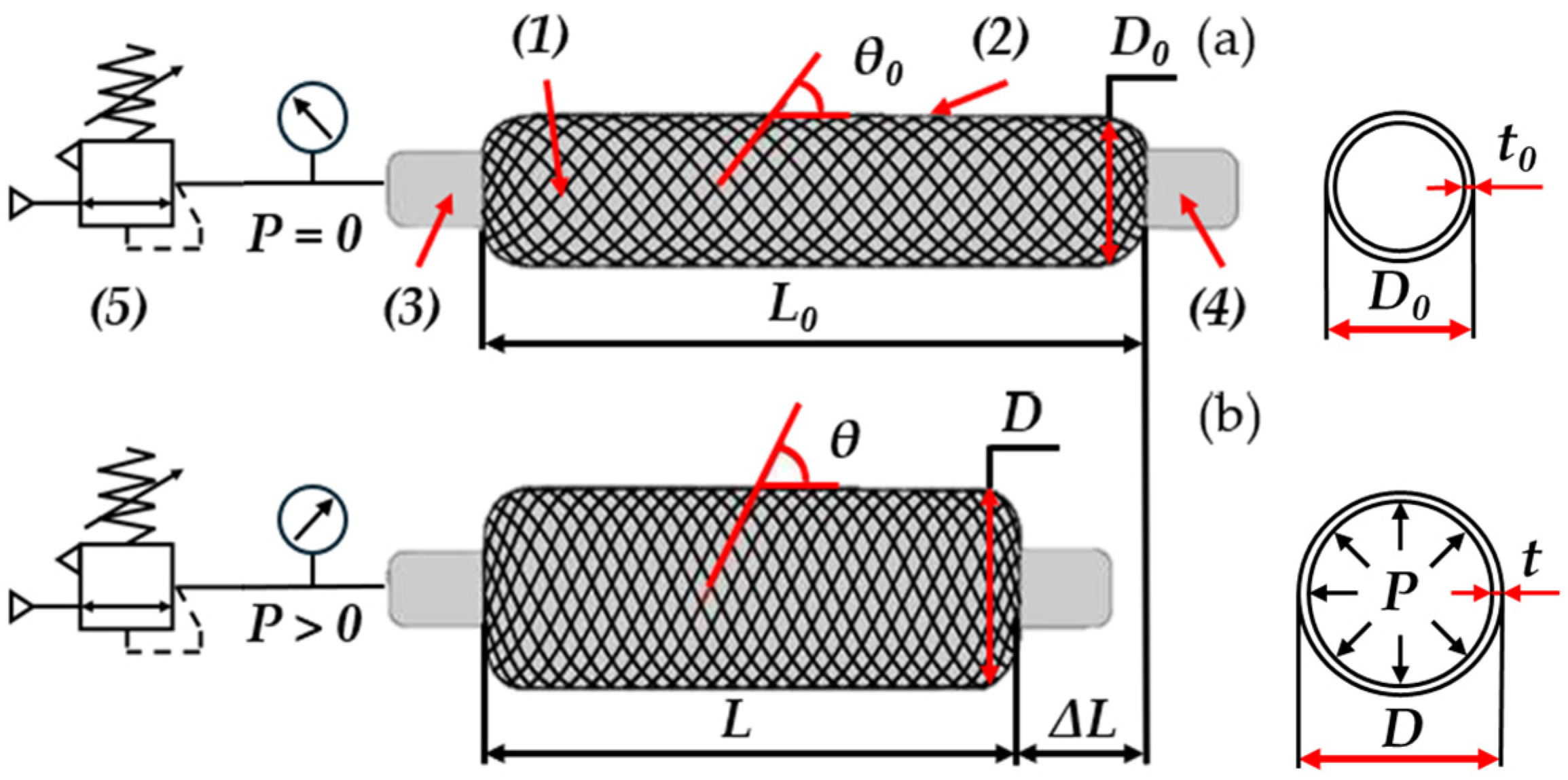
2.1. Technical Description of the MKM

As seen in Figure 1, an MKM consists of an inner tube made of hyperelastic material (1), a fiber reinforcement (2), one end for constraining and pressurization (3), and another end for application of payload or exerting pull forces (4). Figure 1a shows the inner diameter at rest (D₀), tube thickness at rest (t₀), initial fiber angle (θ₀), and initial length (L₀). An actuated state of the MKM is shown in Figure 1b with an indication of the current diameter (D), the actual thickness (t), the fiber inclination angle (θ), the final length (L), the variation in length (ΔL), and the pressure (P). In Figure 1, P is set by a precision pressure regulator (5) equipped with the exhaust port. Under pressurization, by the helical positioning of the inextensible braided fibers of the external reinforcement that act as a pantograph, the MKM radially expands, resulting in an axial shortening of its length. As P increases, the fiber angle θ increases. ΔL results in a shortening ratio (ε), according to Equation (1).

$$\epsilon ={\displaystyle \frac{\Delta L}{L_0}}·100\%$$

(1)

ε is one of the parameters strictly correlated to the force exerted by the muscle using the feeding pressure. The most adopted formulation of the force, defined by Chou and Hannaford in [28], is expressed by Equation (2) and is related to ε.

$$F={\displaystyle \frac{\pi ·{D_0}^2·P}{4}}·{\left({\displaystyle \frac{1}{\sin {\theta }_0}}\right)}^2·\left[3·{\left(1-\epsilon \right)}^2·{cos}^2{\theta }_0-1\right]$$

(2)

This formulation was employed, as it uses the same geometric and functional parameters used for ANN training, as detailed below. If both ends are constrained, force starts to be linearly exerted with the feeding pressure; in the case of a load applied to the MKM, the shortening depends on the feeding pressure for a given external load; in the case of a null load applied to the MKM, until the shortening is free, the MKM does not develop force. Thus, it is essential to understand how the geometric and functional parameters influence the developed force, as described in the following sections.

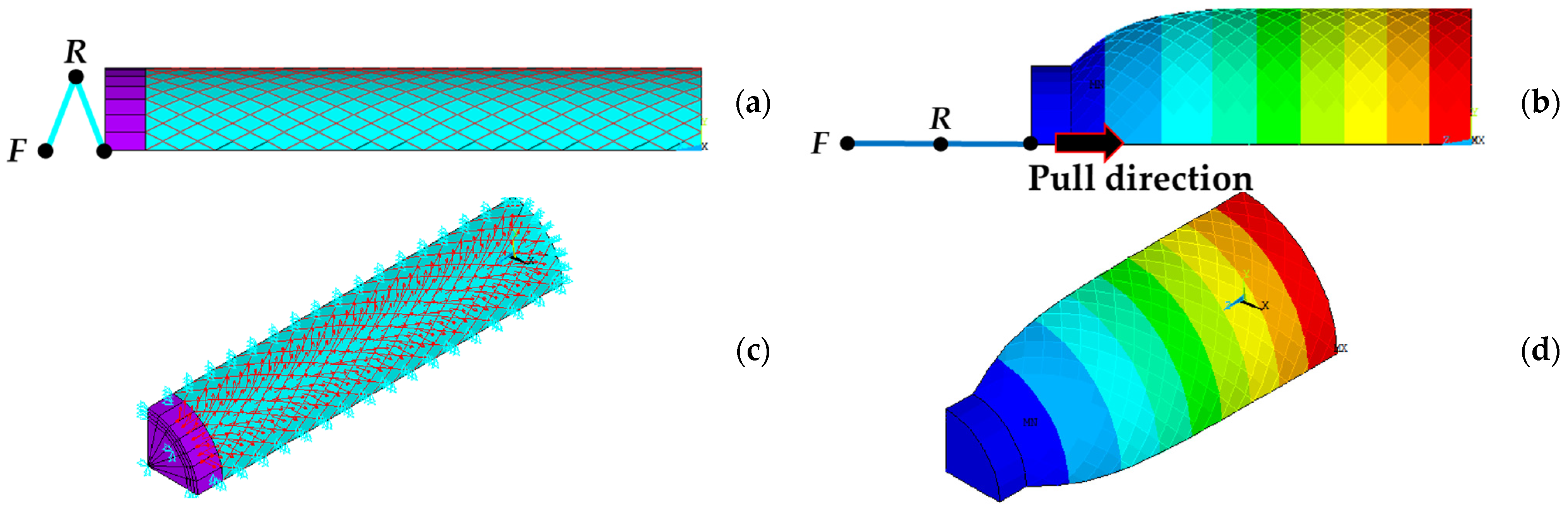
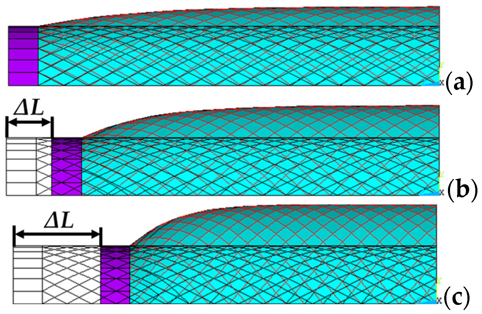
2.2. Numerical Simulations

A 3D non-linear parametric finite element (FE) model was realized to predict the MKM behavior and determine how the muscle-developed force is correlated with its geometric and functional parameters. The FE model was the same as described and experimentally validated in a previous work [40]. The length at rest of the MKM was fixed at 282 mm. Starting from the original model, new models were built for different diameter, thickness, and shortening ratio values, as explained in the following section. Below is a summary of the settings adopted in numerical simulations.

A two-parameter Mooney–Rivlin model was adopted to describe the mechanical behavior of the silicone rubber Silastic S (Reschimica, Barberino Tavarnelle, Italy), which the inner tube was made of. The incompressible hyperelastic strain energy function (W) for this model is reported below:

$$W=C_{10}·\left(I_1-3\right)+C_{01}\left(I_2-3\right)$$

(3)

C₁₀ and C₀₁ have been experimentally identified in [47] and are equal to 0.0694 MPa and 0.0628 MPa, respectively. I₁ and I₂ are the first and second invariants, calculated as functions of the principal stretches (${\lambda }_1$, ${\lambda }_2$, and ${\lambda }_3$):

$$I_1={{\lambda }_1}^2+{{\lambda }_2}^2+{{\lambda }_3}^2$$

(4)

$$I_2={{\lambda }_1}^2·{{\lambda }_2}^2+{{\lambda }_2}^2·{{\lambda }_3}^2+{{\lambda }_3}^2·{{\lambda }_1}^2$$

(5)

Only one-eighth of the geometry is modelled, adding double symmetry, both with respect to the axis of the muscle and the midsection. A joint mechanism was modelled to adjust the maximum shortening, as shown in Figure 2a. This mechanism consists of a three-hinged arch of truss elements connected by sharing the same node (node R). The truss elements were modelled with the LINK180 elements of the Ansys library. The initial and displaced configuration for the links is reported in light and dark blue in Figure 2a,b, respectively. One end of the mechanism is fixed (node F), and the other is connected to the MKM movable part (see Video S1). Thus, the fixed end reacts to the developed force from MKM. All the nodes at the MKM’s left end (purple in Figure 2c) cannot move horizontally. A script written in MATLAB 2024b defines the model components. Non-linear analysis was performed, imposing the Newton–Raphson method within the ANSYS Mechanical APDL 2024. Friction, hysteresis, and time-dependent behavior are neglected. For example, an isometric view of the total deformation for a simulation is shown in Figure 2d, displaying also the braided fibers.

The pressure was incrementally applied, and the reaction force at a fixed point of the mechanism was observed for each fixed ε. In Figure 3a–c, the undeformed and deformed configurations for different ε are shown. This stepwise application of pressure enabled a detailed observation of how MKM responds to several operational conditions.

3. Regression Algorithms

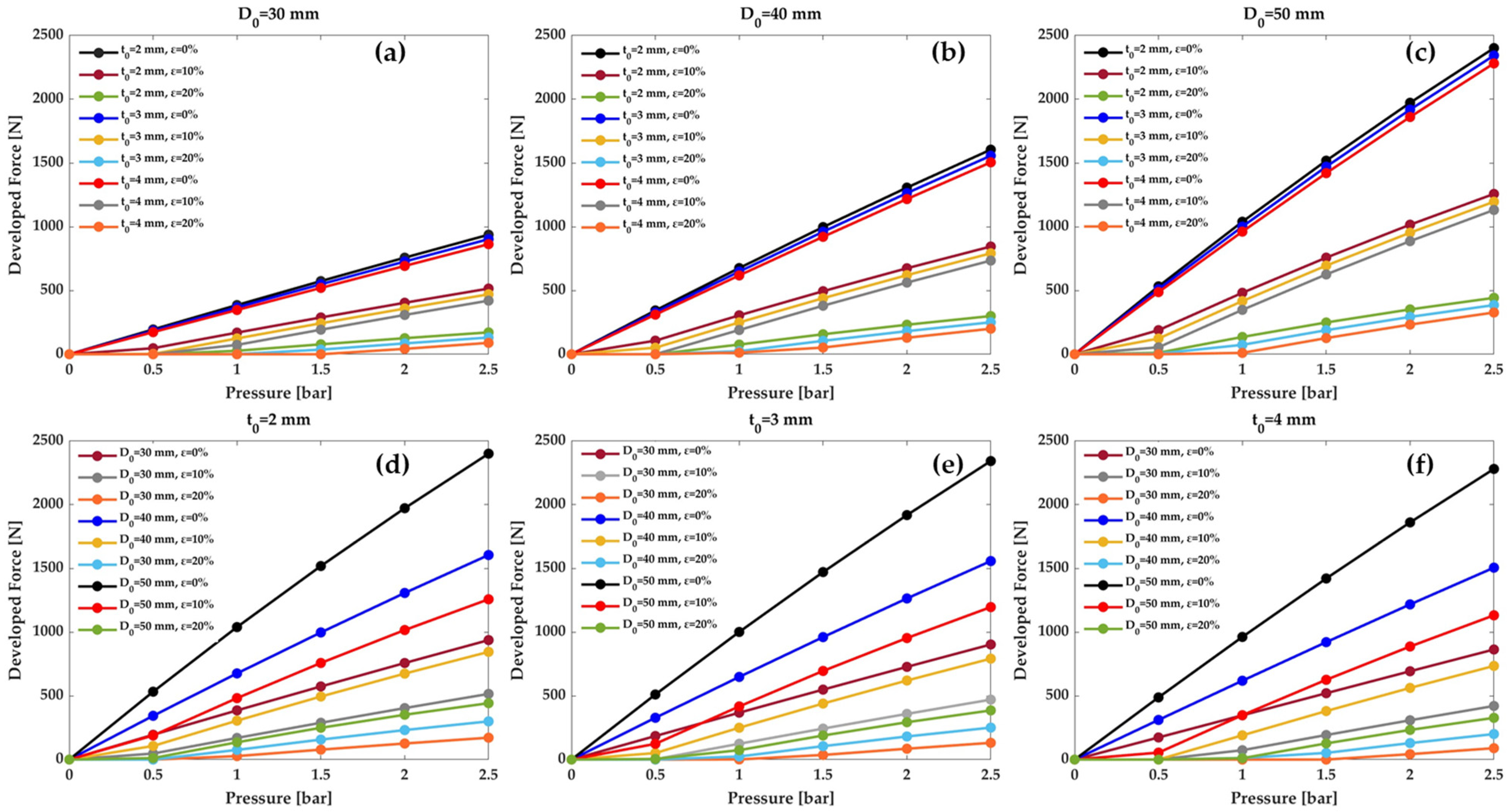
3.1. MKM Dataset Construction

According to the procedure described in the previous Section, and for each numerical model, some preliminary simulations were carried out to evaluate the maximum shortening and pressure that ensure the convergence of the numerical solution. Hence, a test campaign was conducted to build the MKM dataset (Table S1). Numerical models were built for six different pressure values, three diameter values, three inner tube thicknesses, and three shortening ratios for 162 simulations. The values adopted for the parameters are shown in

Table 1. Geometric and functional parameters with the values used to create the MKM dataset.

Name	Symbol	Values	Unit
Pressure	P	0.0–0.5–1.0–1.5–2.0–2.5	bar
Diameter	D0	30–40–50	mm
Thickness	t0	2–3–4	mm
Shortening Ratio	ε	0–10–20	%

with the symbol and relative units.

The numerical results are plotted in Figure 4a–f. The developed force increases linearly with P for any MKM geometry. Similarly, an increase in D₀ of the tube increases the thrust surface and, consequently, the pull force. Moreover, the higher t₀ of the tube results in more significant energy loss to deform it. Finally, an increase in the ε results in more shortening before exerting a pulling force; thus, a loss of energy implies a lower-developed force.

3.2. Training and Validation of the ANNs

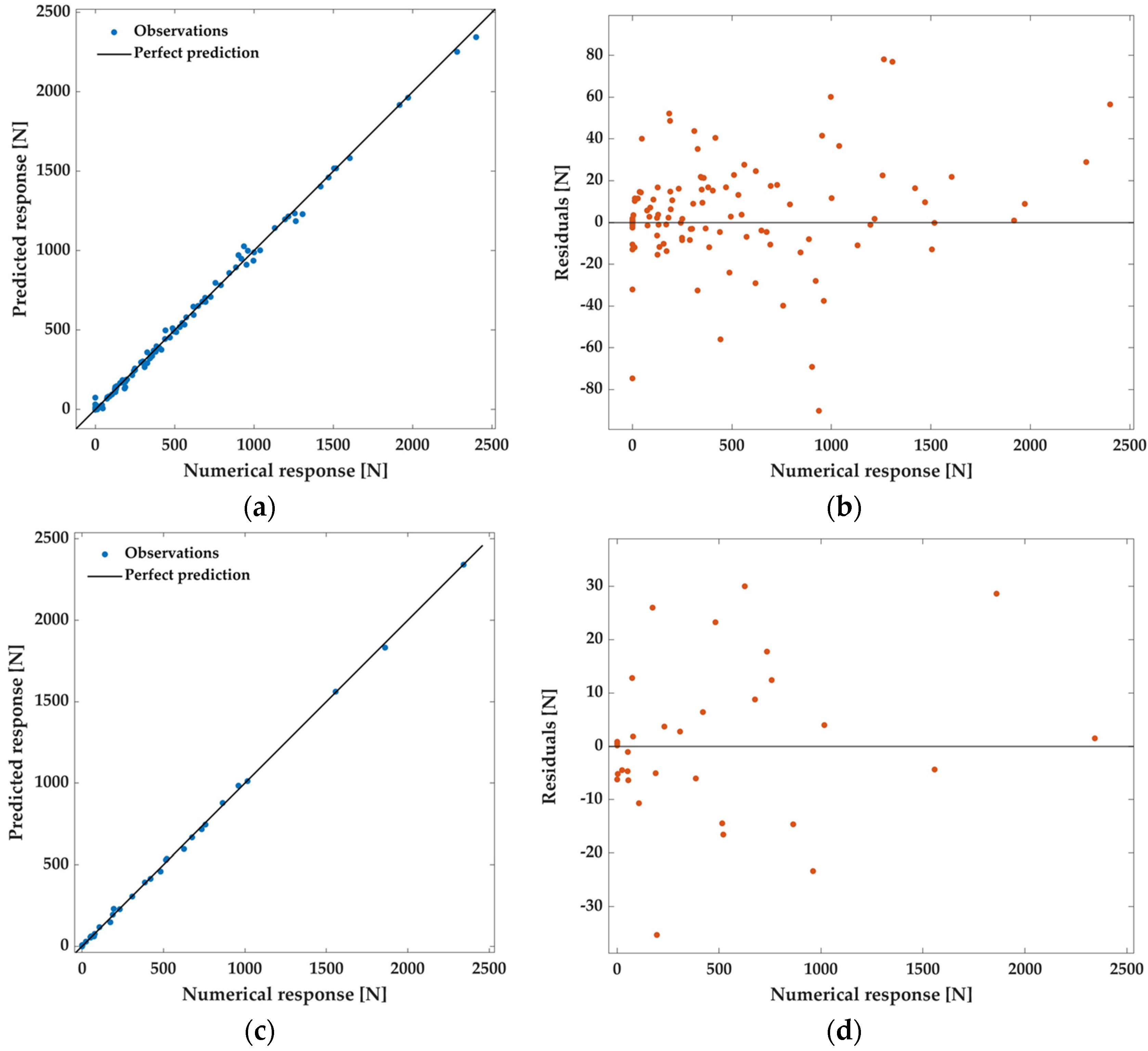
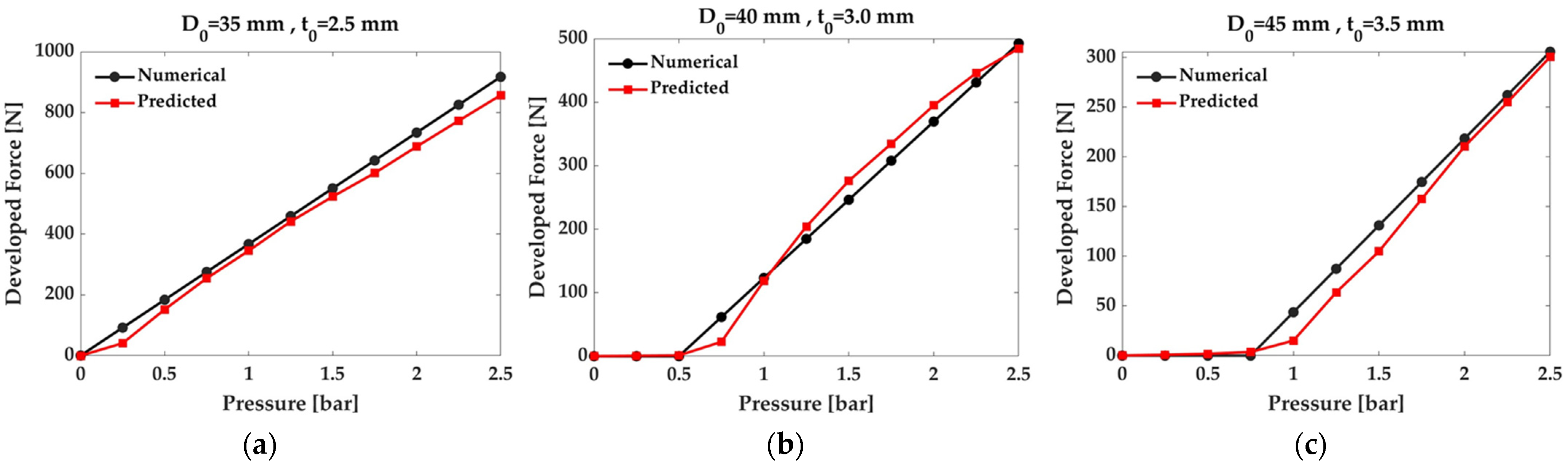
The choice of ML algorithm depends on the problem’s nature, the dataset’s size, and computational constraints. For complex problems with large amounts of data, ANNs are powerful. At the same time, models such as Support Vector Machines and Gaussian Process Regression may be more suitable for small and structured datasets. The latter offers a good trade-off between accuracy and interpretability, while regression models are useful for rapid and interpretable analyses. In addition, regression models are suitable for linear relationships between variables, but their accuracy decreases in the presence of nonlinearities. For these reasons, after creating the MKM dataset, ANNs [48] were trained to identify the most accurate algorithm. The input and output data were normalized in the range [0, 1] to fit the values to a common scale. In this way, there was a more balanced contribution of parameters, leading to more accurate and reliable results and faster convergence.

The training was conducted with the Regression Learning Toolbox of MATLAB R2024b. Data were divided into 80% for training and 20% for validation. Further tests were then performed, as shown in Section 3.3. Different ANNs were tested to identify the best algorithm. ANNs differ in hyper-parameters, number of layers, layer size, and activation functions. Specifically, ANNs can have 1, 2, or 3 layers, a 25, 50, or 100-layer size, and an activation function Rectified Linear Unit (ReLU), hyperbolic tangent (tanh), or sigmoid. The activation function determines whether a neuron in the ANN should be activated or deactivated, thus influencing the neuron’s contribution in predicting the output of the ANN. During the training phase, the choice of activation function is fundamental to ensure good convergence and not hinder the ANN’s learning. Depending on the input and output data, some activation functions may be more suitable than others. An inadequate choice could lead to constantly active or always switched-off neurons, compromising the network’s ability to learn correctly.

Table 2. Performance results for ANNs with different hyperparameters.

Number	Number of Layers	Layer Size	Activation Function	Training RMSE [N]	Validation RMSE [N]
1	1	25	ReLU	66.46	36.51
2	2	25	ReLU	31.84	15.98
3	3	25	ReLU	30.57	14.31
4	1	50	ReLU	34.78	15.52
5	2	50	ReLU	25.59	11.84
6	3	50	ReLU	23.92	8.04
7	1	100	ReLU	27.37	13.78
8	2	100	ReLU	24.29	8.81
9	3	100	ReLU	21.31	7.30
10	1	25	Tanh	363.05	421.37
11	2	25	Tanh	327.30	381.03
12	3	25	Tanh	478.53	593.68
13	1	50	Tanh	329.54	243.02
14	2	50	Tanh	322.29	353.34
15	3	50	Tanh	358.68	738.01
16	1	100	Tanh	307.44	162.88
17	2	100	Tanh	285.92	295.67
18	3	100	Tanh	283.17	280.60
19	1	25	Sigmoid	119.34	81.380
20	2	25	Sigmoid	293.05	386.00
21	3	25	Sigmoid	462.55	448.94
22	1	50	Sigmoid	118.98	69.744
23	2	50	Sigmoid	258.03	123.71
24	3	50	Sigmoid	277.91	403.58
25	1	100	Sigmoid	117.57	79.710
26	2	100	Sigmoid	213.76	202.86
27	3	100	Sigmoid	241.46	230.19

shows the results in terms of RMSE in training and validation. The RMSE is defined as the standard deviation of the residuals, according to Equation (6):

$$RMSE=\sqrt{\sum _{i=1}^n{\displaystyle \frac{{\left(F_{num}-F_{pre}\right)}^2}{n}}}$$

(6)

where $F_{num}$ and $F_{pre}$ are the numerical and the predicted force, respectively, and $n$ is the number of observations.

Different metrics can be used to analyze the performance of an ANN. However, the RMSE has several advantages: the square elevation of the residuals prevents positive and negative values from canceling each other out; furthermore, this parameter amplifies errors of a larger value, allowing methods with more significant errors to be discarded; finally, the RMSE has the same unit of measurement as the original one, so it is easily interpreted. Ideally, an RMSE value of 0 indicates a perfect match between the measured response and that predicted by the algorithm.

In Table 2, the ANN with the lowest RMSE is composed of three layers with 100 neurons and a ReLU activation function. Figure 5a shows the comparison between the predicted and numerical responses for the trials used for training. The values cluster near the bisector of the first quadrant, showing low deviations. To better understand the errors made, Figure 5b shows the residuals (difference between true and predicted responses) as a function of numerical responses. An error is made with ANN’s predictions at zero pressure for a developed force of 0 N. However, this poses no problem, as it will never work at such low pressures. Anyway, in this range of the force (0–2400 N), the limited values of the residuals justify the possible use of ANN in the predictions. Thus, the ANN can predict responses of the developed forces as a function of the combinations of the four chosen parameters.

Turning to the validation, in Figure 5c,d, the plots of the comparison between the predicted and numerical response and the residuals as a function of the numerical response are presented. In this case, the residuals are limited, and the maximum absolute error is at most 38 N. Once again, the ANN can predict the numerical response with a small absolute error.

3.3. Test

To test the ANN predictions under different conditions, three MKM numerical models were simulated with combinations of geometric and functional parameters not used in constructing the MKM dataset. The three MKMs were denoted as I, II, and III, respectively. The I has a diameter of 35 mm, a thickness of 2.5 mm, and ε of 5.0%; the II has a diameter of 40 mm, a thickness of 3.0, and ε of 15.0%; finally, the III has a diameter of 45 mm, a thickness of 3.5 mm, and ε of 20.0%.

Table 3. Comparison between developed numerical and predicted forces for MKMs used in the test with absolute and percentage errors as a function of feeding pressure.

MKM	Pressure	Numerical Force	Predicted Force	Absolute Error	Percentage Error
	[bar]	[N]	[N]	[bar]	[%]
I	0.00	0.00	−0.48	0.48	0.05%
	0.25	91.73	40.51	51.22	5.58%
	0.50	183.46	151.58	31.88	3.48%
	0.75	275.18	254.12	21.06	2.30%
	1.00	366.91	344.84	22.07	2.41%
	1.25	458.64	441.17	17.47	1.90%
	1.50	550.37	523.11	27.26	2.97%
	1.75	642.10	600.59	41.51	4.52%
	2.0	733.82	687.79	46.03	5.02%
	2.25	825.55	772.96	52.59	5.73%
	2.50	917.28	857.18	60.10	6.55%
II	0.00	0.00	0.21	−0.21	−0.04%
	0.25	0.00	0.71	−0.71	−0.14%
	0.50	0.07	1.23	−1.16	−0.24%
	0.75	61.64	22.6	39.04	7.92%
	1.00	123.21	118.54	4.67	0.95%
	1.25	184.78	204.18	−19.40	−3.94%
	1.50	246.35	276.19	−29.85	−6.06%
	1.75	307.91	334.66	−26.75	−5.43%
	2.0	369.48	395.04	−25.56	−5.19%
	2.25	431.05	445.84	−14.79	−3.00%
	2.50	492.62	484.63	7.99	1.62%
III	0.00	0.00	0.11	−0.11	−0.04%
	0.25	0.00	0.88	−0.88	−0.29%
	0.50	0.00	1.94	−1.94	−0.63%
	0.75	0.04	3.61	−3.57	−1.17%
	1.00	43.70	15.14	28.56	9.34%
	1.25	87.37	63.66	23.71	7.76%
	1.50	131.03	104.93	26.10	8.54%
	1.75	174.70	157.69	17.01	5.56%
	2.00	218.36	210.4	7.96	2.60%
	2.25	262.03	254.74	7.29	2.38%
	2.50	305.69	300.61	5.08	1.66%

shows the values of the developed forces evaluated numerically and predicted by the ANN with their absolute and percentage errors (${Err}_{\%}$). The latter was assessed according to Equation (7). The analyses were conducted for pressures in the range of 0.00 to 2.50 bar, with increments of 0.25 bar.

$${Err}_{\%}={\displaystyle \frac{F_{num}-F_{pre}}{max \left(F_{num}\right)}}$$

(7)

It is noted that the ANN predictions can be accepted even for these three geometries and with the chosen functional parameter values. This will avoid re-running numerical simulations in the future by enabling ANN to directly predict the developed force of the MKM as a function of parameters. One of the main advantages is the speed of ANN without waiting for the numerical simulation results. For example, the ANN required 131 ms to predict the forces developed by the three MKMs.

The results are plotted in Figure 6a–c and show that the maximum absolute error of 60.10 N is committed for the I MKM at a pressure of 2.50 bar. However, in this test, the maximum developed force is 918.28 N, producing an acceptable percentage error of 6.55%. The maximum percentage error for the III MKM at a pressure of 1.00 bar is 9.34%. Again, the error is acceptable. Indeed, the developed force is low, starting from a shortening ratio of 20.0%. For this configuration, the working pressures are higher to have higher pulling forces.

A deeper analysis reveals that errors are primarily concentrated in two specific pressure ranges. The forces are generally small at low pressures, preventing the actuator from being used for these pressure values. However, percentage error calculations become more sensitive, leading to higher percentage values. On the other hand, at high pressures, the actuators generate much larger forces, resulting in more pronounced absolute errors (e.g., up to 60.10 N for the I MKM). Despite this, these errors represent only a small fraction of the total forces, which explains the relatively low percentage of errors under these conditions. This behavior is particularly relevant for applications requiring high performance, where the model maintains high relative accuracy. Results obtained for the three pneumatic actuators confirm the effectiveness of the ANN-based approach, showing a good balance between accuracy, efficiency, and flexibility. The advantage of ANNs is that they learn directly from the data, establishing correlations between input and output. This is fundamental, as there is no need to identify a specific law; on the other hand, a potential disadvantage is that it can sometimes be difficult to maintain physical correlation, obtaining physically acceptable results. It is important to compare different ANNs, as done by varying the hyperparameters, because the results show how ANNs can learn the physical phenomena underlying the process. For example, it was observed that regardless of the geometry of the MKM and the hyperparameters of the ANNs, an increase in pressure always corresponds to an increase in the force developed by the system. The same happens with an increase in the diameter of the MKM, increasing the thrust section. Thus, ANNs can understand the physical phenomena underlying the process.

Expanding the dataset to cover a broader range of operating conditions could further refine this aspect. Another key advantage of the predictive ANN is the significant time savings compared to perform numerical simulations. The ability to quickly estimate the developed forces by pneumatic actuators represents a strategic benefit, especially in deciding the geometric and functional parameters according to the field of use and application. While the results are promising, there are possibilities for improvement. Expanding the dataset with additional combinations of geometric and functional parameters and incorporating alternative materials or variable payloads could enhance the model’s ability to generalize working conditions.

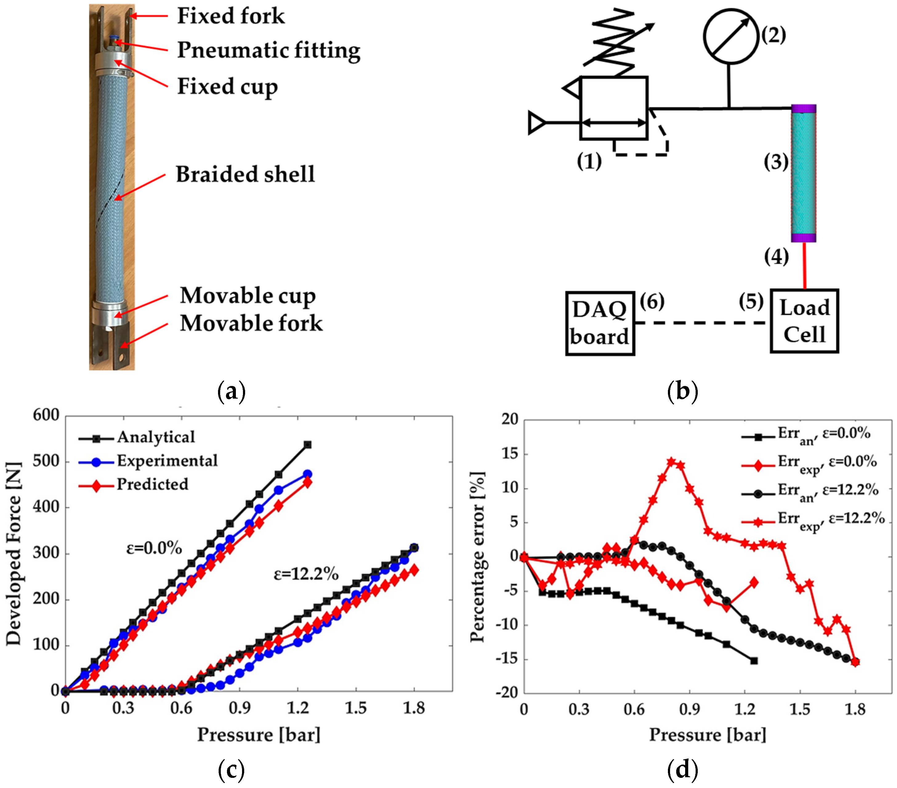
4. Experimental Validation

A comparison between the experimental forces of an MKM in quasi-static tests and those predicted by ANN is given in this section. The prototype shown in Figure 7a has an inner diameter, thickness, and working length of 30, 3, and 282 mm, respectively, and a total mass of 0.598 kg. One of the cups is fixed and used for pressurization, while the other is movable. The adopted test bench for the measurements is in Figure 7b. It consists of (1) precision pressure regulator SMC IR1220-N01-A (f.s. 4.0 bar, SMC Corporation, Tokyo, Japan) to adjust the pressure within the actuator, (2) manometer (f.s. 2. 5 bar, NUOVA FIMA, Invorio, Italy), (3) tested MKM, (4) threaded rod joined to the lower end and a plate, acting like a movable nut along the rod to fix the length of the MKM (fixing the shortening ratio), (5) analog transducers TCA10 tension/compression load cell (full scale ±10 kg; output signal ±10Vdc; nominal sensitivity 2 mV/V; sensitivity tolerance ≤ ±0.1%, AEP transducers, Modena, Italy) to measure the developed force by the actuator, and (6) a National Instruments USB-6001 data acquisition board, to acquire the load cell signal with a frequency of 10 Hz.

Figure 7c compares the measured forces of the MKM, the force predicted by the formulation in Equation (2), and those predicted by ANN for a shortening ratio of 0.0% and 12.2%. The ANN underestimates the forces for an ε = 0.0%, committing negative percentage errors, as plotted in Figure 7d. The maximum percentage error is about −8.2% concerning the measured forces, and −16.3% with respect to the predictions of the analytical formulation. For the tests with ε = 12.2%, the maximum percentage errors are −15.3% and 15.9% compared to measured force and predicted by formulation, respectively. These errors demonstrate the feasibility of using the ANN to choose geometric and functional parameters based on the forces to be developed with MKM. Furthermore, the results confirm how the ANN learned the physical phenomenon behind the data used for training. Indeed, it can be seen from Figure 7c that ANN can predict the linear correlation between developed force and feeding pressure, which is in line with Hannaford’s formulation and experimental data.

5. Conclusions

In this work, a hybrid approach between FEAs and ML algorithms to predict the developed force of MKMs was proposed. Based on the numerical results of 162 simulations carried out with FE models of MKMs for different combinations of geometric and functional parameters, the MKM dataset was created. Hence, the dataset was adopted to train ANNs to identify the most accurate one for predicting the developed forces.

The best algorithm was a three-layer network, with 100 neurons per layer and a ReLU activation function. The predictions of this network were compared with numerical forces on three MKMs that were not included in the dataset construction. The maximum percentage errors for the I, II, and III MKMs were 6.55%, 7.92%, and 9.34%, respectively. These errors are considered acceptable, especially given the advantage of predicting the developed force by the MKM without the need to set up and wait for numerical simulation results, significantly reducing time requirements. Also, the comparison with the realized and tested prototype confirms that the ANN can predict the developed forces, facilitating the choice of geometrical and functional parameters according to the required force.

This work highlights how the application of ML techniques can lead to significant advancements in the prediction and design of MKMs. Future developments will consider additional parameters not included in the network training, such as using different hyper-elastic silicone rubbers, alternative reinforcement materials, and the MKM length that changes the developed force. Hence, new numerical models will be built and simulated, and the results will be added to the dataset, which will be expanded with additional parameter combinations to extend the range of applications and improve the ANN’s predictive accuracy. This study marks a significant step forward in the mechanical design of the MKM based on the field of use and application.

References

1. Shintake, J.; Cacucciolo, V.; Floreano, D.; Shea, H. Soft Robotic Grippers. Adv. Mater. 2018, 30, 1707035. [Google Scholar] [CrossRef] [PubMed]
2. Kalita, B.; Leonessa, A.; Dwivedy, S.K. A Review on the Development of Pneumatic Artificial Muscle Actuators: Force Model and Application. Actuators 2022, 11, 288. [Google Scholar] [CrossRef]
3. Antonelli, M.G.; Beomonte Zobel, P.; Mattei, E.; Stampone, N. A Methodology for the Mechanical Design of Pneumatic Joints Using Artificial Neural Networks. Appl. Sci. 2024, 14, 8324. [Google Scholar] [CrossRef]
4. Antonelli, M.G.; Beomonte Zobel, P.; Mattei, E.; Stampone, N. Mechanical Design, Manufacturing, and Testing of a Soft Pneumatic Actuator with a Reconfigurable Modular Reinforcement. Robotics 2024, 13, 165. [Google Scholar] [CrossRef]
5. Moreki, A. Polish artificial pneumatic muscles. In Proceedings of the 7th International Conference on Climbing and Walking Robot, Karlsruhe, Germany, 24–26 September 2001. [Google Scholar]
6. Shinohara, H.; Nakamura, T. Derivation of a mathematical model for pneumatic artificial muscles. IFAC Proc. Vol. 2006, 39, 266–270. [Google Scholar] [CrossRef]
7. Schulte, H. The characteristics of the McKibben artificial muscle. In The Application of External Power in Prosthetics and Orthotics; National Academy of Sciences-National Research Council: Washington, DC, USA, 1961; pp. 94–115. [Google Scholar]
8. Gavrilović, M.M.; Marić, M.R. Positional servo-mechanism activated by artificial muscles. Med. Biol. Eng. 1969, 7, 77–82. [Google Scholar] [CrossRef] [PubMed]
9. Yariott, J.M. Fluid Actuator. U.S. Patent 3,645,173, 29 February 1972. [Google Scholar]
10. Morin, A.H. Elastic Diaphragm. U.S. Patent 2,642,091, 16 June 1953. [Google Scholar]
11. Paynter, H.M. Hyperboloid of Revolution Fluid-Driven Tension Actuators and Method of Making. U.S. Patent 4,721,030, 26 January 1988. [Google Scholar]
12. Han, K.; Kim, N.H.; Shin, D. A novel soft pneumatic artificial muscle with high-contraction ratio. Soft Robot. 2018, 5, 554–566. [Google Scholar] [CrossRef]
13. Daerden, F.; Lefeber, D. The concept and design of pleated pneumatic artificial muscles. Int. J. Fluid Power 2001, 2, 41–50. [Google Scholar] [CrossRef]
14. Daerden, F.; Lefeber, D. Pneumatic artificial muscles: Actuators for robotics and automation. Eur. J. Mech. Environ. Eng. 2002, 47, 11–21. [Google Scholar]
15. Terryn, S.; Brancart, J.; Lefeber, D.; Van Assche, G.; Vanderborght, B. A pneumatic artificial muscle manufactured out of self-healing polymers that can repair macroscopic damages. IEEE Robot. Autom. Lett. 2017, 3, 16–21. [Google Scholar] [CrossRef]
16. Belforte, G.; Eula, G.; Ivanov, A.; Sirolli, S. Soft Pneumatic Actuators for Rehabilitation. Actuators 2014, 3, 84–106. [Google Scholar] [CrossRef]
17. Noritsugu, T.; Takaiawa, M.; Sasaki, D. Development of a pneumatic rubber artificial muscle for human support applications. In Proceedings of the 9th Scandinavia International Conference on Fluid Power, Linkoping, Sweden, 1–3 June 2005. [Google Scholar]
18. Hannford, B.; Winters, J.M. Actuators properties and movement control: Biological and technological models. In Multiple Muscle Systems; Winters, J., Woo, S., Eds.; Springer: New York, NY, USA, 1990; pp. 101–120. [Google Scholar]
19. Chen, C.-T.; Lien, W.-Y.; Chen, C.-T.; Wu, Y.-C. Implementation of an Upper-Limb Exoskeleton Robot Driven by Pneumatic Muscle Actuators for Rehabilitation. Actuators 2020, 9, 106. [Google Scholar] [CrossRef]
20. Waycaster, G.; Wu, S.K.; Shen, X. Design and control of a pneumatic artificial muscle actuated above-knee prosthesis. J. Med. Devices 2011, 5, 031003. [Google Scholar] [CrossRef]
21. Fantoni, G.; Santochi, M.; Dini, G.; Tracht, K.; Scholz-Reiter, B.; Fleischer, J.; Lien, T.K.; Seliger, G.; Reinhart, G.; Franke, J.; et al. Grasping devices and methods in automated production processes. CIRP Ann. 2014, 63, 679–701. [Google Scholar] [CrossRef]
22. Giannaccini, M.E.; Georgilas, I.; Horsfield, I.; Peiris, B.; Lenz, A.; Pipe, A.G.; Dogramadzi, S. A variable compliance, soft gripper. Auton. Robot. 2014, 36, 93–107. [Google Scholar] [CrossRef]
23. Verrelst, B.; Van Ham, R.; Vanderborght, B.; Lefeber, D.; Daerden, F.; Van Damme, M. Second generation pleated pneumatic artificial muscle and its robotic applications. Adv. Robot. 2006, 20, 783–805. [Google Scholar] [CrossRef]
24. Martens, M.; Seel, T.; Zawatzki, J.; Boblan, I. A novel framework for a systematic integration of pneumatic-muscle-actuator-driven joints into robotic systems via a torque control interface. Actuators 2018, 7, 82. [Google Scholar] [CrossRef]
25. Koter, K.; Fracczak, L.; Chojnacka, K.; Jabłoński, K.; Zarychta, S.; Podsędkowski, L. Snake robot based on McKibben Pneumatic Artificial Muscles. In Proceedings of the 15th Conference on Dynamical Systems Theory and Applications DSTA, Lodz, Poland, 2–5 December 2019. [Google Scholar]
26. Iwata, K.; Suzumori, K.; Wakimoto, S. A method of designing and fabricating McKibben muscles driven by 7 MPa hydraulics. Int. J. Autom. Technol. 2012, 6, 482–487. [Google Scholar] [CrossRef]
27. Kobayashi, R.; Nabae, H.; Mao, Z.; Endo, G.; Suzumori, K. Enhancement of Thin McKibben Muscle Durability Under Repetitive Actuation in a Bent State. IEEE Robot. Autom. Lett. 2024, 9, 9685–9692. [Google Scholar] [CrossRef]
28. Chou, C.P.; Hannaford, B. Measurement and modeling of McKibben pneumatic artificial muscles. IEEE Trans. Robot. Autom. 1996, 12, 90–102. [Google Scholar] [CrossRef]
29. Tondu, B.; Lopez, P. Modeling and control of McKibben artificial muscle robot actuators. IEEE Control. Syst. Mag. 2000, 20, 15–38. [Google Scholar]
30. Marechal, L.; Balland, P.; Lindenroth, L.; Petrou, F.; Kontovounisios, C.; Bello, F. Toward a Common Framework and Database of Materials for Soft Robotics. Soft Robot. 2021, 8, 284–297. [Google Scholar] [CrossRef]
31. Inada, R.; Tsuruhara, S.; Ito, K. Precise Displacement Control of Tap-Water-Driven Muscle Using Adaptive Model Predictive Control with Hysteresis Compensation. JFPS Int. J. Fluid Power Syst. 2022, 15, 78–85. [Google Scholar] [CrossRef]
32. Tsuruhara, S.; Ito, K. Data-Driven Model-Free Adaptive Displacement Control for Tap-Water-Driven Artificial Muscle and Parameter Design Using Virtual Reference Feedback Tuning. J. Robot. Mechatron. 2022, 34, 664–676. [Google Scholar] [CrossRef]
33. Serres, J.; Reynolds, D.; Phillips, C.; Rogers, D.; Repperger, D. Characterisation of a pneumatic muscle test station with two dynamic plants in cascade. Comput. Methods Biomech. Biomed. Eng. 2010, 13, 11–18. [Google Scholar] [CrossRef]
34. Serres, J.; Reynolds, D.; Phillips, C.; Gerschutz, M.; Repperger, D. Characterisation of a phenomenological model for commercial pneumatic muscle actuators. Comput. Methods Biomech. Biomed. Eng. 2009, 12, 423–430. [Google Scholar] [CrossRef]
35. Kalita, B.; Dwivedy, S. Nonlinear dynamics of a parametrically excited pneumatic artificial muscle (PAM) actuator with simultaneous resonance condition. Mech. Mach. Theory 2019, 135, 281–297. [Google Scholar] [CrossRef]
36. Kalita, B.; Dwivedy, S. Dynamic analysis of pneumatic artificial muscle (PAM) actuator for rehabilitation with principal parametric resonance condition. Nonlinear Dyn. 2019, 97, 2271–2289. [Google Scholar] [CrossRef]
37. Wickramatunge, K.C.; Leephakpreeda, T. Study on mechanical behaviors of pneumatic artificial muscle. Int. J. Eng. Sci. 2010, 48, 188–198. [Google Scholar] [CrossRef]
38. Wickramatunge, K.C.; Leephakpreeda, T. Empirical modeling of dynamic behaviors of pneumatic artificial muscle actuators. ISA Trans. 2013, 52, 825–834. [Google Scholar] [CrossRef]
39. Antonelli, M.G.; Beomonte Zobel, P.; D’Ambrogio, W.; Durante, F.; Raparelli, T. An Analytical Formula for Designing Mckibben Pneumatic Muscles. Int. J. Mech. Technol. 2018, 9, 320–337. [Google Scholar]
40. Antonelli, M.G.; Beomonte Zobel, P.; Durante, F.; Raparelli, T. Numerical modelling and experimental validation of a McKibben pneumatic muscle actuator. J. Intell. Mater. Syst. Struct. 2017, 28, 2737–2748. [Google Scholar] [CrossRef]
41. Antonelli, M.G.; Beomonte Zobel, P.; De Marcellis, A.; Palange, E. Design and Characterization of a Mckibben Pneumatic Muscle Prototype with an Embedded Capacitive Length Transducer. Machines 2022, 10, 1156. [Google Scholar] [CrossRef]
42. Kotkas, L.; Zhurkin, N.; Donskoy, A.; Zharkovskij, A. Design and Mathematical Modeling of a Pneumatic Artificial Muscle-Actuated System for Industrial Manipulators. Machines 2022, 10, 885. [Google Scholar] [CrossRef]
43. Yang, H.D.; Greczek, B.T.; Asbeck, A.T. Modeling and Analysis of a High-Displacement Pneumatic Artificial Muscle with Integrated Sensing. Front. Robot. AI 2019, 5, 136. [Google Scholar] [CrossRef]
44. Wang, G.; Wereley, N.M.; Pillsbury, T. Non-linear quasi-static model of pneumatic artificial muscle actuators. J. Intell. Mater. Syst. Struct. 2014, 26, 541–553. [Google Scholar] [CrossRef]
45. Bennington, M.J.; Wang, T.; Yin, J.; Bergbreiter, S.; Majidi, C.; Webster-Wood, V.A. Design and Characterization of Viscoelastic McKibben Actuators with Tunable Force-Velocity Curves. In Proceedings of the 2023 IEEE International Conference on Soft Robotics (RoboSoft), Singapore, 3–7 April 2023; pp. 1–7. [Google Scholar]
46. Slightam, J.E.; Nagurka, M.L. Modeling of Pneumatic Artificial Muscle with Kinetic Friction and Sliding Mode Control. In Proceedings of the 2018 Annual American Control Conference (ACC), Milwaukee, WI, USA, 27–29 June 2018; pp. 3342–3347. [Google Scholar]
47. Durante, F.; Antonelli, M.G.; Zobel, P.; Raparelli, T. Development of a Straight Fibers Pneumatic Muscle. Int. J. Autom. Technol. 2018, 12, 413–423. [Google Scholar] [CrossRef]
48. Nunes da Silva, I.; Hernane Spatti, D.; Andrade Flauzino, R.; Bartocci Liboni, L.H.; Franco dos Reis Alves, S. Artificial Neural Networks: A Practical Course; Springer: Cham, Switzerland, 2016. [Google Scholar]
Figure 1. Schematic of the MKM: (a) at rest (P = 0); (b) actuated (P > 0). Components of an MKM: (1) inner tube made of hyperelastic material, (2) fiber reinforcement, (3) end for constraining and pressurization, (4) opposite end to exert pull force, (5) precision pressure regulator.
Actuators 14 00153 g001
Figure 2. (a) FE model of the MKM with the three-hinged arch in the initial position (light blue); (b) total deformation after pressurization with the three-hinged arch in the final position (dark blue); (c) isometric view of the FE model with constraints and loads; (d) isometric view of the total deformation.
Actuators 14 00153 g002
Figure 3. Undeformed and deformed state at: (a) ε equal to 0.0% (ΔL equal to 0.0 mm); (b) ε equal to 10.0% (ΔL equal to 28.2 mm); (c) ε equal to 20.0% (ΔL equal to 56.4 mm).
Actuators 14 00153 g003
Figure 4. Developed forces as a function of the pressure for: (a) D0 = 30 mm; (b) D0 = 40 mm; (c) D0 = 50 mm; (d) t0 = 2 mm; (e) t0 = 3 mm; (f) t0 = 4 mm.
Actuators 14 00153 g004
Figure 5. Training and validation results: (a) comparison between predicted and numerical developed forces in training; (b) residual vs numerical response in training; (c) comparison between predicted and numerical developed forces in validation; (d) residual vs numerical response in validation.
Actuators 14 00153 g005
Figure 6. Comparison between numerical and predicted results as a function of the pressure for an MKM with: (a) D0 = 35 mm, t0 = 2.5 mm, and ε = 5.0% (ΔL equal to 14.1 mm); (b) D0 = 40 mm, t0 = 3.0 mm and ε = 15.0% (ΔL equal to 42.3 mm); (c) D0 = 45 mm, t0 = 3.5 mm, and ε = 20.0% (ΔL equal to 56.4 mm).
Actuators 14 00153 g006
Figure 7. (a) Tested MKM with D0 = 30 mm, t0 = 3.0 mm, and L0 = 282 mm and an indication of its components; (b) adopted test bench with the pneumatic circuit: (1) precision pressure regulator, (2) manometer, (3) actuator, (4) threaded rod joined to the lower end and a plate, (5) load cell, (6) data acquisition board; (c) experimental, analytical, and predicted developed forces for the MKM with D0 = 24.0 mm, t0 = 3.0 mm, and L0 = 282 mm; (d) percentage error as a function of the pressure.
Actuators 14 00153 g007