Adaptive Nonlinear Friction Compensation for Pneumatically Driven Follower in Force-Projecting Bilateral Control

Abstract

Force-projecting bilateral control is an effective method for enhancing the positioning rigidity and stability of teleoperation systems equipped with compliant pneumatically driven followers. However, friction in the pneumatic actuation mechanism has caused a deterioration in force reproducibility between the leader and follower. To solve this problem, this study proposes a practical method of nonlinear friction compensation in force-projecting bilateral control to improve the force reproducibility. The proposed method generates two friction compensation forces: one based on the target admittance velocity from the leader and the other based on the actual velocity of the follower. These forces are seamlessly switched according to the dynamic state of the system to compensate for the follower’s driving force. This enables improved force reproducibility in any motion states of the system while maintaining the advantage of force-projecting bilateral control, which eliminates the need for external force measurement on the follower side. Experiments were conducted using a 1-DOF bilateral control device consisting of an electric linear motor and a pneumatic cylinder, including free motion and contact operations with two types of environments, demonstrating the effectiveness of the proposed method.

1. Introduction

1.1. Research Background

Since pneumatic manipulators have advantages such as their lightness, flexibility, high environmental resistance, and high affinity for humans, they have been adopted for surgical robots [1,2,3,4] and construction machinery operating robots [5,6]. These manipulation systems perform teleoperation using the leader–follower method. If such a system can not only match positions but also transmit a sense of force to the operator, it will enable safer and more precise teleoperation. For this purpose, a teleoperation method called bilateral control, which simultaneously controls the position and force of the controller (leader) and the robot (follower), is effective. However, when the conventional bilateral control method is applied to a pneumatic robot teleoperation system, large position error and instability become serious problems.

In bilateral control, prominent control methods such as symmetric type, force-reflecting type, and force-feedback type have been developed since early times, and various research efforts have been made to address different challenges. One of the main research issues in bilateral control was preventing instability caused by communication delay between the leader and follower. Various approaches have been developed to address this issue [7,8,9,10,11,12]. Another critical issue is force and position matching between the leader and the follower; that is, the transparency of bilateral control systems. Yokokohji et al. [13,14] proposed the four-channel bilateral control method. This method enables the force and position to be matched simultaneously with high accuracy by using a total of four types of information, namely position and force information from both the leader and follower. Ohnishi et al. [15,16] proposed a force sensorless acceleration control method for actuators and applied it to four-channel bilateral control, achieving high transparency even when the dynamics between leader and follower were different. Furthermore, the issue of external force measurement on the follower side is also a critical factor that complicates the realization of transparent and stable bilateral control. It is often the case that force sensors cannot be installed, especially on the follower, due to the robot’s working environment or space constraints. Ohnishi et al. [17,18] proposed a method of external force estimation using disturbance observer based on the motion and driving force of actuators. In addition, recent studies have actively developed bilateral control methods that can estimate environmental parameters on the follower side in real time using machine learning techniques [19,20,21]. However, all of the aforementioned methods are designed for systems with electric manipulators that have sufficient control responsiveness and positioning rigidity. Therefore, it is difficult to directly apply them to flexible and low-responsive pneumatic-driven manipulators. Very few studies have addressed the performance enhancement of bilateral systems with low control rigidity and responsiveness, such as pneumatic manipulators.

To find a practical solution to this issue, our research group focused on the force-projecting bilateral control (force-projecting type) [22]. Force-projecting type is a control method in which the operational force of the leader is directly projected onto the follower, and the follower position is reproduced by the leader. Therefore, this method does not require external force information on the follower side, and there is no need to install a force sensor or estimate the force. In addition, this method relies solely on the leader for positioning stiffness. As a result, even if the follower has low positioning stiffness, the entire control system can achieve high positioning stiffness as long as the leader has high positioning stiffness. In our previous studies [23,24,25], it was demonstrated that force-projecting type significantly improves the positioning rigidity and stability of bilateral control using a 1-DOF teleoperation system with a pneumatic-driven follower. However, since the operational force of the leader is projected directly onto the follower, the follower dynamics must be provided by the operational force of the leader. Therefore, the operational feeling during free motion becomes heavy. The main factor that worsens the operational feeling is the sliding friction of the follower mechanism. In our previous study [26], we found that the environmental reaction force was buried in the friction force of the pneumatic follower, which reduced the accuracy of the operator’s identification of the environment. Therefore, a method is needed to improve the operational feel by appropriately compensating for the friction of the pneumatic-driven follower while maintaining the advantages of the force-projecting type in terms of positioning rigidity and stability. Developing this method directly contributes to improving the force reproducibility between the leader and the follower.

1.2. Related Works

There have been many studies estimating and compensating for friction in actuators. The most typical compensation method is the disturbance observer-based disturbance compensation method [27,28,29], which aims to ensure that the actuator follows the reference trajectory without being affected by disturbances such as actuator friction or external forces. However, this method requires control at the acceleration level of the system and assumes a high-speed control response from the actuator. Therefore, when applied to slow-response pneumatic manipulators, system stability becomes a major issue.

Modeling and identifying actuator friction have also been actively studied. These methods require the construction of appropriate models of individual actuators for geared machine tools [30], electric motors [31,32], and hydraulic drive systems [33]. The modeling and identification methods for nonlinear friction have been applied to nonlinear dynamic compensation and robust adaptive control in robot arm trajectory control [34,35] and to adaptive model predictive control in vehicle transmissions [36]. These techniques are designed for automatic control applications where the reference trajectory is predetermined, but they are not directly applicable to bilateral control. Regarding pneumatic actuators, Schindele et al. [37] proposed a friction compensation method for pneumatic rodless cylinders, demonstrating its effectiveness in actuator position control. However, the applicability of the proposed method to bilateral control still remains unclear because the study did not provide investigation and discussion from the perspective of force control.

The latest trend shows that deep neural networks are increasingly being used for the identification of nonlinear dynamic models to realize sensorless external force estimation [38]. Xiao et al. [39] proposed an improved LuGre friction model that considers the coupled effects of load torque and joint motion and applied it to the impedance trajectory control of a robotic arm. While the expressive capability of nonlinear friction models is superior, their approach does not target bilateral control in teleoperation. As a result, no compensation method is provided that takes into account the dynamic state of the leader device. Phuong et al. [40] constructed a precise reaction force observer using an LSTM deep neural network and demonstrated its effectiveness through simulations. However, their evaluation did not consider environmental model variations, and stability issues are anticipated when feeding back the estimated external force in an actual system. Therefore, applying this method to a pneumatic drive system would be challenging.

1.3. Research Design

1.3.1. Objective

Considering the background mentioned above, this study aims at developing a method to improve the force reproducibility in the force-projecting type with a pneumatic follower device by compensating for its nonlinear friction while maintaining the advantages of high positioning rigidity and system stability.

In the teleoperation system targeted in this study, the following conditions are assumed.

(A1)

Since the leader is operated by a human operator, it has a high design flexibility and can be driven by an electric motor or equipped with a force sensor.

(A2)

Depending on the application, the follower is mechanically or electromagnetically exposed to harsh working environments or requires high flexibility and ease of operation. It is difficult to mount a force sensor on the follower due to its small size and working environment. Thus, a pneumatic manipulator with high back-drivability is suitable for the follower device.

Examples of such leader–follower systems include the medical robot system and construction machine control robot system described above, as well as systems for use in explosion-proof environments and actuation in an anechoic chamber.

1.3.2. Contributions and Novelty

To maintain high transparency [41] in bilateral control, this study considers not only the internal dynamic state of the manipulator but also the relationship with the operational force and the environmental reaction force. The proposed method is an algorithm of Adaptive Nonlinear Friction Compensation (ANFC), which identifies the overall dynamic state of the system to adaptively compensate for the nonlinear friction forces of the pneumatic follower according to each state. In this study, the proposed ANFC is implemented in a 1-DOF electric leader–pneumatic follower system, and its effectiveness is evaluated through experiments by comparing the control performance with that of the normal force-projecting type.

1.3.3. Organization of This Paper

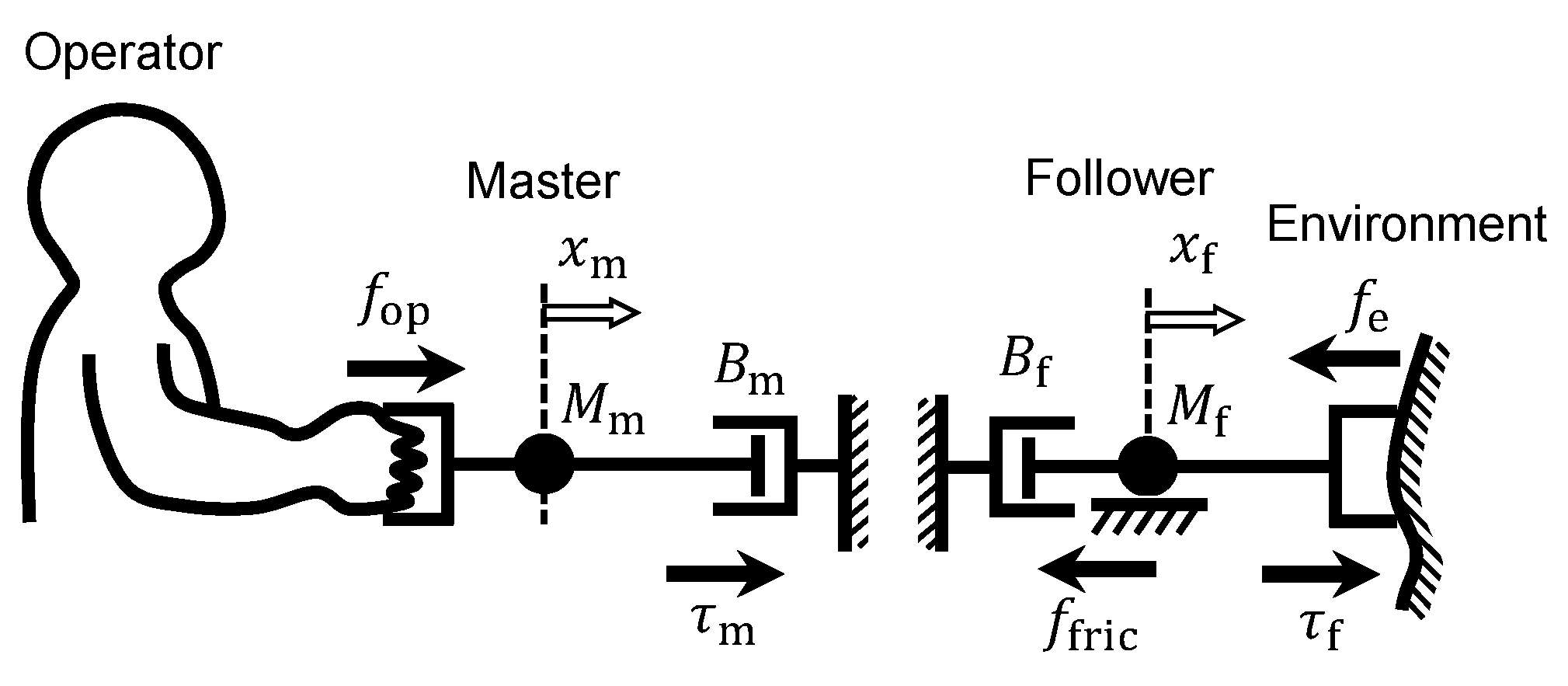
Section 1 (this section) describes the research background, reviews the related works, and presents the objective and novelty of this study. In Section 2, the dynamic model of a 1-DOF bilateral teleoperation system with friction force is presented, followed by an explanation of the fundamental theory regarding force reproducibility in the force-projecting type. Section 3 presents the concept and method of the proposed ANFC, including algorithm implementation. Section 4 provides the configuration of the 1-DOF bilateral teleoperation experiment system and the controller design with ANFC. Section 5 shows the experimental results: transient responses and frequency responses. Section 6 evaluates the essential effectiveness of the proposed method, discusses its advantages compared to related works, and considers potential approaches for further performance improvement. Finally, Section 7 provides the conclusion, summarizing the findings of this study.

2. System Modeling

A 1-DOF leader–follower system is modeled in this section. In this paper, we consider a leader–follower system, as illustrated in Figure 1. The physical quantities represented by each symbol are listed in

Table 1. Symbols and descriptions.

Description	Symbol	Unit
First-order derivative	$\dot{◯}$
Second-order derivative	$\ddot{◯}$
Estimated value	$\widehat{◯}$
Reference value	${◯}^{\mathrm{ref}}$
Time	t	[s]
Leader position	$x_{\mathrm{m}}$	[mm]
Follower position	$x_{\mathrm{f}}$	[mm]
Position error between leader and follower	$x_{\mathrm{e}}$	[mm]
Leader driving force	${\tau }_{\mathrm{m}}$	[N]
Follower driving force	${\tau }_{\mathrm{f}}$	[N]
Operational force at leader	$f_{\mathrm{op}}$	[N]
Environmental reaction force at follower	$f_{\mathrm{e}}$	[N]
Nonlinear friction force of follower	$f_{\mathrm{fric}}$	[N]
Mass of leader	$M_{\mathrm{m}}$	[kg]
Mass of follower	$M_{\mathrm{f}}$	[kg]
Viscous coefficient of leader	$B_{\mathrm{m}}$	[Ns/mm]
Viscous coefficient of follower	$B_{\mathrm{f}}$	[Ns/mm]
Coulomb friction force	$D_{\mathrm{f}}$	[N]

. The leader has mass and viscosity in its dynamics. On the other hand, the follower, which is assumed to be pneumatically driven, has a nonlinear friction force $f_{\mathrm{fric}}$ in addition to mass and viscosity in its dynamics. The equation of motion for the leader is expressed by Equation (1).

$$\begin{array}{ccc}\hfill M_{\mathrm{m}}{\ddot{x}}_{\mathrm{m}}& =& f_{\mathrm{op}}+{\tau }_{\mathrm{m}}-B_{\mathrm{m}}{\dot{x}}_{\mathrm{m}}\hfill \end{array}$$

(1)

The operational force $f_{\mathrm{op}}$ applied by the operator, the leader driving force ${\tau }_{\mathrm{m}}$, and the leader viscous force $B_{\mathrm{m}}{\dot{x}}_{\mathrm{m}}$ act on the leader, which has a mass $M_{\mathrm{m}}$. These forces generate an acceleration ${\ddot{x}}_{\mathrm{m}}$. The equation of motion for the follower is expressed by Equation (2).

$$\begin{array}{ccc}\hfill M_{\mathrm{f}}{\ddot{x}}_{\mathrm{f}}& =& f_{\mathrm{e}}+{\tau }_{\mathrm{f}}-B_{\mathrm{f}}{\dot{x}}_{\mathrm{f}}-f_{\mathrm{fric}}\hfill \end{array}$$

(2)

The environmental reaction force $f_{\mathrm{e}}$, the follower driving force ${\tau }_{\mathrm{f}}$, the follower viscous force $B_{\mathrm{f}}{\dot{x}}_{\mathrm{f}}$, and the follower friction force $f_{\mathrm{fric}}$ act on the follower, which has a mass $M_{\mathrm{f}}$. The follower friction force $f_{\mathrm{fric}}$ is modeled as a combination of the Coulomb friction force and the static friction force. It is divided into cases, as shown in Equation (3).

$$\begin{array}{ccc}\hfill f_{\mathrm{fric}}& =& \left\{\begin{array}{cc}{D}_{\mathrm{f}}\mathrm{sgn}\left({\dot{\mathrm{x}}}_{\mathrm{f}}\right)\hfill & ({\dot{x}}_{\mathrm{f}}\ne 0),\hfill \\ f_{\mathrm{e}}+{\tau }_{\mathrm{f}}\hfill & ({\dot{x}}_{\mathrm{f}}=0).\hfill \end{array}\right.\hfill \end{array}$$

(3)

When an object is in motion, the Coulomb friction force $D_{\mathrm{f}}$ acts in the direction opposite to the velocity of the object. Therefore, by applying the equation of motion for the follower (2), we obtain the following equation:

$$\begin{array}{ccc}\hfill M_{\mathrm{f}}{\ddot{x}}_{\mathrm{f}}+B_{\mathrm{f}}{\dot{x}}_{\mathrm{f}}+D_{\mathrm{f}}\mathrm{sgn}\left({\dot{\mathrm{x}}}_{\mathrm{f}}\right)& =& f_{\mathrm{e}}+{\tau }_{\mathrm{f}}({\dot{x}}_{\mathrm{f}}\ne 0)\hfill \end{array}$$

(4)

On the other hand, when the follower is stationary, a static friction force acts on it. The state of the follower is determined by the sum of the follower driving force ${\tau }_{\mathrm{f}}$ and the environmental reaction force $f_{\mathrm{e}}$. When the magnitude of the sum $f_{\mathrm{e}}+{\tau }_{\mathrm{f}}$ is less than the maximum static friction force $F_{\max }$, the static friction force acts to cancel $f_{\mathrm{e}}+{\tau }_{\mathrm{f}}$. At this time, the follower is stationary (i.e., its velocity is 0), and the following equation is obtained from the equation of motion (2).

$$\begin{array}{ccc}\hfill M_{\mathrm{f}}{\ddot{x}}_{\mathrm{f}}& =& 0({\dot{x}}_{\mathrm{f}}=0)\hfill \end{array}$$

(5)

In the force-projecting type, the smaller the static friction on the follower side, the more desirable it is. Therefore, a pneumatic actuator, which has high backdrivability, is suitable. When the magnitude of $f_{\mathrm{e}}+{\tau }_{\mathrm{f}}$ exceeds the maximum static friction force $F_{\max }$, the follower begins to move, and the Coulomb friction force $D_{\mathrm{f}}$ acts in the direction opposite to its velocity.

Next, we define the transparency of the bilateral control response and describe the properties of the force-projecting type. For transparent (i.e., ideal) bilateral control, Lawrence [41] states that the following relation holds:

$$\begin{array}{ccc}\hfill {\dot{x}}_{\mathrm{m}}& =& {\dot{x}}_{\mathrm{f}}\hfill \end{array}$$

(6)

$$\begin{array}{ccc}\hfill f_{\mathrm{op}}& =& -f_{\mathrm{e}}\hfill \end{array}$$

(7)

Equation (6) shows that the leader and follower have equal velocities, so their motions coincide. Equation (7) represents the state in which the action–reaction law holds between the operator and the environment because the direction of the operational force and the environmental reaction force are opposite and their magnitudes are equal.

Figure 2 shows the basic structure of the force-projecting type, which directly projects the operational force to the follower driving force and reproduces the follower position at the leader. Namely, the follower does not have a position controller and only needs to transmit its current position to the leader, eliminating the need for external force measurement. These characteristics provide significant advantages for pneumatic driving systems with low positioning rigidity and high back-drivability. The impact of the follower dynamics on this control method is theoretically explained based on the transparency [41].

First, Equation (6), which represents motion trajectory matching, can be considered to be realized with high performance. This is because position control is handled by the leader side, which has sufficient control characteristics. Then, for Equation (7), which represents the force input/output consistency (reproducibility), assuming a system in which the leader and follower scales are equal, the follower driving force is as follows:

$$\begin{array}{ccc}\hfill {\tau }_{\mathrm{f}}& =& f_{\mathrm{op}}\hfill \end{array}$$

(8)

Substituting this into the follower’s equation of motion yields the following:

$$\begin{array}{ccc}\hfill f_{\mathrm{op}}& =& -f_{\mathrm{e}}+M_{\mathrm{f}}{\ddot{x}}_{\mathrm{f}}+B_{\mathrm{f}}{\dot{x}}_{\mathrm{f}}+f_{\mathrm{fric}}.\hfill \end{array}$$

(9)

Comparing this with Equation (7), we see that an extra force term due to follower dynamics $M_{\mathrm{f}}{\ddot{x}}_{\mathrm{f}}+B_{\mathrm{f}}{\dot{x}}_{\mathrm{f}}+f_{\mathrm{fric}}$ is included. This causes the heavy leader operational force in the force-projecting type. Here, adding a compensation term based on the follower dynamics model to the follower driving force ${\tau }_{\mathrm{f}}$ in Equation (8), we obtain the following equation:

$$\begin{array}{ccc}\hfill {\tau }_{\mathrm{f}}& =& f_{\mathrm{op}}+{\widehat{M}}_{\mathrm{f}}{\ddot{x}}_{\mathrm{f}}+{\widehat{B}}_{\mathrm{f}}{\dot{x}}_{\mathrm{f}}+{\widehat{f}}_{\mathrm{fric}}\hfill \end{array}$$

(10)

Substituting this into the follower equation of motion (2) yields the following:

$$\begin{array}{ccc}\hfill f_{\mathrm{op}}& =& -f_{\mathrm{e}}+\left(M_{\mathrm{f}}{\ddot{x}}_{\mathrm{f}}+B_{\mathrm{f}}{\dot{x}}_{\mathrm{f}}+f_{\mathrm{fric}}\right)-\left({\widehat{M}}_{\mathrm{f}}{\ddot{x}}_{\mathrm{f}}+{\widehat{B}}_{\mathrm{f}}{\dot{x}}_{\mathrm{f}}+{\widehat{f}}_{\mathrm{fric}}\right).\hfill \end{array}$$

(11)

If the follower dynamics model can be accurately identified, then the follower dynamics term and the compensation term cancel each other out. Then, the force reproducibility given in Equation (7) holds. Since mass and viscosity can be accurately identified in a dynamics model, this study focuses on a compensation method for the remaining nonlinear friction force.

3. Proposal of Adaptive Nonlinear Friction Compensation Method

3.1. Concept

This section describes the proposed ANFC algorithm. Let ${\tau }_{\mathrm{c}}$ denote the dynamics compensation term presented in the previous section.

$$\begin{array}{ccc}\hfill {\tau }_{\mathrm{c}}& =& {\widehat{M}}_{\mathrm{f}}{\ddot{x}}_{\mathrm{f}}+{\widehat{B}}_{\mathrm{f}}{\dot{x}}_{\mathrm{f}}+{\widehat{f}}_{\mathrm{fric}}\hfill \end{array}$$

(12)

The inertia term in the first term is ignored because the mass of the pneumatic cylinder, which is assumed for the follower, is small. Here, the key point is how to compensate ${\widehat{f}}_{\mathrm{fric}}$ in the third term. The nonlinear friction force composed of Coulomb friction and static friction is modeled as shown in Equation (3), i.e., it is determined by the environmental reaction force. However, it is difficult to directly estimate the environmental reaction force buried in the friction force without a force sensor. Fundamentally, the force-projecting type does not require external force detection at the follower side, which is a major advantage. Moreover, feedback should be prevented in the system when external force is applied to a follower with low responsiveness. Therefore, we consider using the leader operational force information in addition to the follower velocity information to identify the acting state of the environmental reaction force. The proposed method uses this information comprehensively as criteria and switches the process of calculating the compensation force of Coulomb friction, assuming that the section of static friction is the transition region.

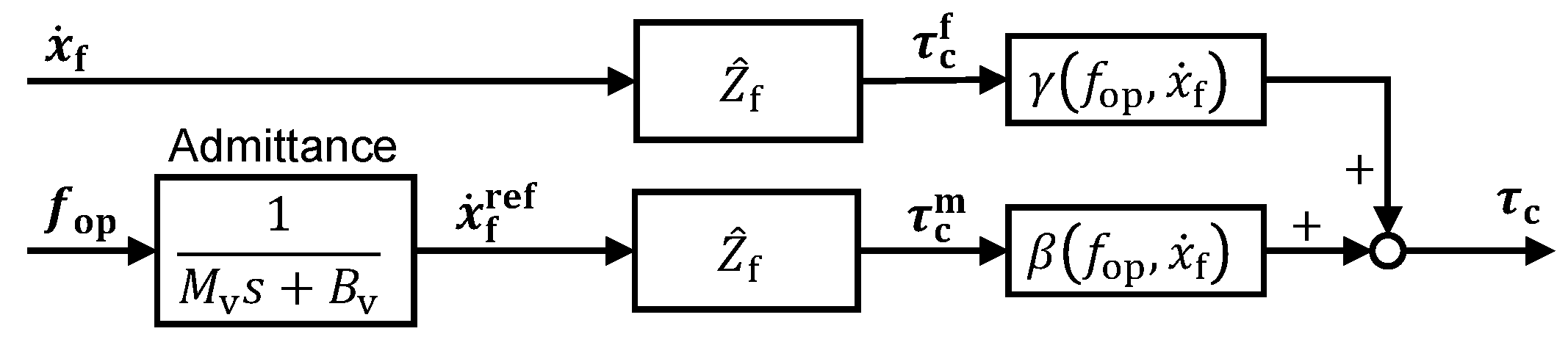
3.2. Scheme of Adaptive Nonlinear Friction Compensation

The computational process of the proposed ANFC is shown in Figure 3 as a block diagram. In a typical position control system, the reference velocity ${\dot{x}}_{\mathrm{f}}^{\mathrm{ref}}$ is often used to compensate for friction forces. However, the proposed compensation method refers to both the reference velocity ${\dot{x}}_{\mathrm{f}}^{\mathrm{ref}}$ and the current velocity ${\dot{x}}_{\mathrm{f}}$, considering the proper functioning in a bilateral system. Here, the follower reference velocity ${\dot{x}}_{\mathrm{f}}^{\mathrm{ref}}$ is calculated by applying the leader operational force $f_{\mathrm{op}}$ to the admittance of the virtual mass $M_{\mathrm{v}}$ and the virtual viscosity $B_{\mathrm{v}}$. The compensation force referring to the follower reference velocity ${\dot{x}}_{\mathrm{f}}^{\mathrm{ref}}$ is denoted as ${\tau }_{\mathrm{c}}^{\mathrm{m}}$, and the compensation force referring to the follower current velocity ${\dot{x}}_{\mathrm{f}}$ is denoted as ${\tau }_{\mathrm{c}}^{\mathrm{f}}$. The final compensation force ${\tau }_{\mathrm{c}}$ is determined by weighting and summing these forces using the mixing ratios $\beta$ and $\gamma$. The mixing ratios $\beta$ and $\gamma$ are determined based on the operating state of the system, and the operating state of the system is identified based on the operational force $f_{\mathrm{op}}$ and the follower velocity ${\dot{x}}_{\mathrm{f}}$. The proposed method is described in detail below.

${\tau }_{\mathrm{c}}^{\mathrm{m}}$ and ${\tau }_{\mathrm{c}}^{\mathrm{f}}$ show the compensation force derived from the reference velocity ${\dot{x}}_{\mathrm{f}}^{\mathrm{ref}}$ and the current velocity ${\dot{x}}_{\mathrm{f}}$, respectively, and is determined using the follower inverse dynamics model ${\widehat{Z}}_{\mathrm{f}}$ as follows:

$$\begin{array}{ccc}\hfill {\tau }_{\mathrm{c}}^{\mathrm{m}}={\widehat{Z}}_{\mathrm{f}}{\dot{x}}_{\mathrm{f}}^{\mathrm{ref}}& =& {\widehat{B}}_{\mathrm{f}}{\dot{x}}_{\mathrm{f}}^{\mathrm{ref}}+\left\{\begin{array}{cc}{\widehat{D}}_{\mathrm{f}}\mathrm{sgn}\left({\dot{\mathrm{x}}}_{\mathrm{f}}^{\mathrm{ref}}\right)\hfill & \left(\right|{\dot{x}}_{\mathrm{f}}^{\mathrm{ref}}|>v_{\lim }),\hfill \\ {\displaystyle \frac{|{\dot{x}}_{\mathrm{f}}^{\mathrm{ref}}|}{v_{\lim }}}{\widehat{D}}_{\mathrm{f}}\mathrm{sgn}\left({\dot{\mathrm{x}}}_{\mathrm{f}}^{\mathrm{ref}}\right)\hfill & \left(\right|{\dot{x}}_{\mathrm{f}}^{\mathrm{ref}}|\le v_{\lim }).\hfill \end{array}\right.\hfill \end{array}$$

(13)

$$\begin{array}{ccc}\hfill {\tau }_{\mathrm{c}}^{\mathrm{f}}={\widehat{Z}}_{\mathrm{f}}\left({\dot{x}}_{\mathrm{f}}\right)& =& {\widehat{B}}_{\mathrm{f}}{\dot{x}}_{\mathrm{f}}+\left\{\begin{array}{cc}{\widehat{D}}_{\mathrm{f}}\mathrm{sgn}\left({\dot{\mathrm{x}}}_{\mathrm{f}}\right)\hfill & \left(\right|{\dot{x}}_{\mathrm{f}}|>v_{\lim }),\hfill \\ {\displaystyle \frac{|{\dot{x}}_{\mathrm{f}}|}{v_{\lim }}}{\widehat{D}}_{\mathrm{f}}\mathrm{sgn}\left({\dot{\mathrm{x}}}_{\mathrm{f}}\right)\hfill & \left(\right|{\dot{x}}_{\mathrm{f}}|\le v_{\lim }).\hfill \end{array}\right.\hfill \end{array}$$

(14)

Here, to prevent the Coulomb friction compensation force from switching discontinuously because of the sign function, the approximation process is carried out such that the Coulomb friction force is reduced linearly at low speeds when the magnitude of the velocity is less than $v_{\lim }(\ge 0)$. After obtaining the compensation terms ${\tau }_{\mathrm{c}}^{\mathrm{m}}$ and ${\tau }_{\mathrm{c}}^{\mathrm{f}}$ from the two types of velocity information using the above equations, the total dynamics compensation to the follower ${\tau }_{\mathrm{c}}$ is determined using the mixing ratios $\beta$ and $\gamma$ as follows:

$$\begin{array}{ccc}\hfill {\tau }_{\mathrm{c}}& =& \beta {\tau }_{\mathrm{c}}^{\mathrm{m}}+\gamma {\tau }_{\mathrm{c}}^{\mathrm{f}}\hfill \end{array}$$

(15)

For a reason that will be explained later, in this method, the compensation force is selectively switched between ${\tau }_{\mathrm{c}}^{\mathrm{m}}$ and ${\tau }_{\mathrm{c}}^{\mathrm{f}}$ depending on the operating state of the system. In order to avoid discontinuous switching of the compensating force, the mixing ratios $\beta$ and $\gamma$ are introduced as smoothing parameters. These can be set arbitrarily. In this study, they are set to maintain the following relationship:

$$\begin{array}{c}\hfill \beta +\gamma =1\end{array}$$

(16)

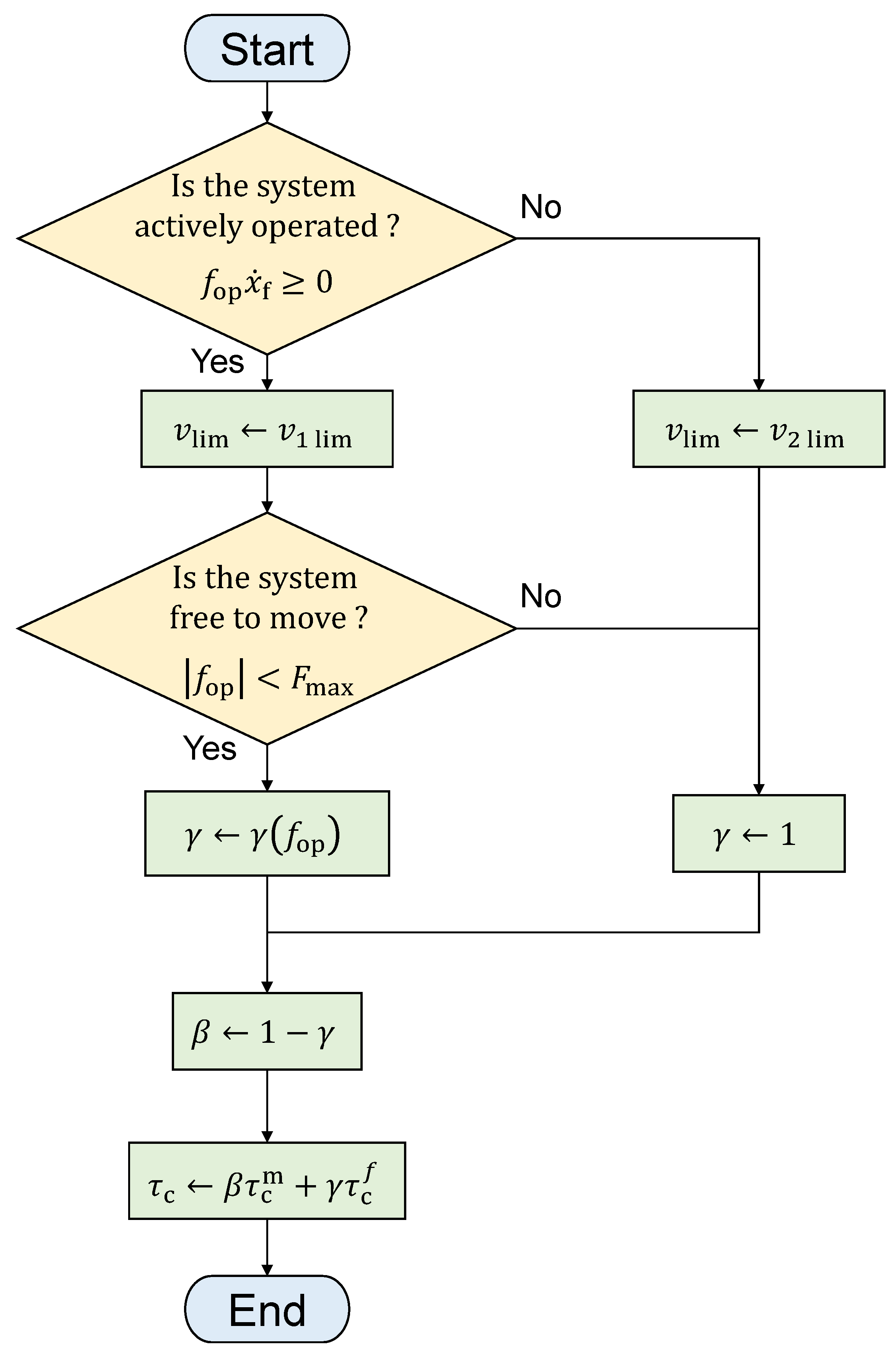
3.3. Setting the Mixing Ratio Parameters

The method used to determine the mixing ratios $\beta$ and $\gamma$ is described. We use the leader operational force $f_{\mathrm{op}}$ and follower current velocity ${\dot{x}}_{\mathrm{f}}$ as parameters to identify the operating state of the system. In the force-projecting type, the follower is in one of the following operating states:

(a)

Stationary state. $(f_{\mathrm{op}}{\dot{x}}_{\mathrm{f}}=0)$,

(b)

Moving in response to the operational force $(f_{\mathrm{op}}{\dot{x}}_{\mathrm{f}}>0)$,

(c)

Being pushed in the direction opposite to the operational force due to the environmental reaction force $(f_{\mathrm{op}}{\dot{x}}_{\mathrm{f}}<0)$.

First, consider the case where the magnitude of the operational force $|f_{\mathrm{op}}|$ is less than the maximum static friction force $F_{\max }$ (i.e., $|f_{\mathrm{op}}|<F_{\max }$). In states (a) and (b), since the environmental reaction force is either zero or very small, the follower can be considered free to move. Therefore, the reference velocity is used $(\gamma =0)$ to predictably compensate for the operating resistance, including static friction. In state (c), given that the follower is moving due to an external force, the current velocity is used to compensate $(\gamma =1)$.

In contrast, consider the case where the magnitude of the operational force $|f_{\mathrm{op}}|$ is greater than or equal to the maximum static friction force $F_{\max }$ (i.e., $|f_{\mathrm{op}}|\ge F_{\max }$). In all states (a), (b) and (c), the manifest environmental reaction force can be considered to be balanced by the operational force and the follower’s dynamic state. If friction compensation is performed with the reference velocity in such a contact state with the environment, the compensation force will not function properly because of the deviation between the reference and current velocities. In other words, the force consistency deteriorates when the environmental reaction force cannot be measured and fed back. For this reason, the current velocity is referenced $(\gamma =1)$ for compensation in all states in this case $\left(\right|f_{\mathrm{op}}|\ge F_{\max })$.

The above policy can be summarized in the following equation.

$$\begin{array}{ccc}\hfill {\gamma }_{\mathrm{ideal}}& =& \left\{\begin{array}{cc}0\hfill & \left(|f_{\mathrm{op}}|<{\widehat{F}}_{\max }\wedge f_{\mathrm{op}}{\dot{x}}_{\mathrm{f}}\ge 0\right),\hfill \\ 1\hfill & \left(|f_{\mathrm{op}}|\ge {\widehat{F}}_{\max }\vee f_{\mathrm{op}}{\dot{x}}_{\mathrm{f}}<0\right).\hfill \end{array}\right.\hfill \end{array}$$

(17)

However, if the parameters are actually varied as in the above equation, the switching will be discontinuous. Thus, a smoothing function is introduced. In this study, the mixing ratio $\gamma$ is set using a cubic function of the absolute value of the operational force $|f_{\mathrm{op}}|$ as follows.

$$\begin{array}{ccc}\hfill \gamma \left(f_{\mathrm{op}}\right)& =& \left\{\begin{array}{cc}{\eta }_3|f_{\mathrm{op}}{|}^3+{\eta }_2|f_{\mathrm{op}}{|}^2+{\eta }_1\left|f_{\mathrm{op}}\right|+{\eta }_0\hfill & \left(|f_{\mathrm{op}}|<{\widehat{F}}_{\max }\wedge f_{\mathrm{op}}{\dot{x}}_{\mathrm{f}}\ge 0\right),\hfill \\ 1\hfill & \left(|f_{\mathrm{op}}|\ge {\widehat{F}}_{\max }\vee f_{\mathrm{op}}{\dot{x}}_{\mathrm{f}}<0\right).\hfill \end{array}\right.\hfill \end{array}$$

(18)

The real coefficients ${\eta }_0$ to ${\eta }_3$ are determined so that this cubic function satisfies the following boundary conditions:

$$\begin{array}{c}\hfill \left\{\begin{array}{c}\gamma \left(0\right)=0,{\displaystyle \frac{d\gamma \left(0\right)}{d|f_{\mathrm{op}}|}}=0,\hfill \\ \gamma \left({\widehat{F}}_{\max }\right)=1,{\displaystyle \frac{d\gamma \left({\widehat{F}}_{\max }\right)}{d|f_{\mathrm{op}}|}}=0.\hfill \end{array}\right.\end{array}$$

(19)

Then, the real coefficients are determined as follows: ${\eta }_0=0,{\eta }_1=0{\eta }_2={\displaystyle \frac{3}{{\widehat{F}}_{\max }^2}}{\eta }_3=-{\displaystyle \frac{2}{{\widehat{F}}_{\max }^3}}$. A profile of this function is shown in Figure 4. Once the mixing ratio $\gamma$ is obtained in this way, the other mixing ratio $\beta$ can be determined by the relationship in Equation (16). Finally, the compensation force can be obtained according to Equation (15).

3.4. Algorithm Implementation

In this section, the implementation of the algorithm defined in the previous section is described. Figure 5 shows a flowchart of the process by which the compensation force ${\tau }_{\mathrm{c}}$ is determined. $\gamma \left(f_{\mathrm{op}}\right)$ in Figure 5 shows the smoothing function in Equation (18). The value of $v_{\lim }$ used in Equations (13) and (14) is set separately depending on whether the operator is actively moving the system $(f_{\mathrm{op}}{\dot{x}}_{\mathrm{f}}\ge 0)$ or the system is being passively moved by the environment $(f_{\mathrm{op}}{\dot{x}}_{\mathrm{f}}<0)$. When the operator is actively moving the system, it is set as $v_{1\lim }$. When the system is being moved passively, it is set as $v_{2\lim }$. The relationship between $v_{1\lim }$ and $v_{2\lim }$ is set as $v_{1\lim }>v_{2\lim }$. This is to prevent the system from becoming unstable due to the unstable operational force when actively operating the system. When the system is being passively moved by the environment, the current velocity is used ($\gamma =1$). When the magnitude of the operational force $|f_{\mathrm{op}}|$ is greater than or equal to the maximum static friction force $F_{\max }$ (i.e., $|f_{\mathrm{op}}|\ge F_{\max }$), the environmental reaction force can be considered to be balanced by the operational force and the follower’s dynamic state. Therefore, the current velocity is referenced $(\gamma =1)$. On the other hand, when the operator is actively moving the system, and when the magnitude of the operational force $|f_{\mathrm{op}}|$ is less than the maximum static friction force $F_{\max }$ (i.e., $|f_{\mathrm{op}}|<F_{\max }$), the follower can be considered free to move. Therefore, the reference velocity is also used $(\gamma =\gamma \left(f_{\mathrm{op}}\right))$. Once the mixing ratio $\gamma$ is obtained, the other mixing ratio $\beta$ can be determined by the relationship in Equation (16). Finally, the compensation force ${\tau }_{\mathrm{c}}$ can be obtained according to Equation (15).

The control parameters of ANFC are defined as shown in

Table 2. Control parameters of ANFC.

Description	Symbol	Value	Unit
Smoothing range $(f_{\mathrm{op}}{\dot{x}}_{\mathrm{f}}\ge 0)$	$v_{1\lim }$	5.0	[mm/s]
Smoothing range $(f_{\mathrm{op}}{\dot{x}}_{\mathrm{f}}<0)$	$v_{2\lim }$	0.20	[mm/s]
Estimated viscous coefficient of follower	${\widehat{B}}_{\mathrm{f}}$	0.030	[Ns/mm]
Estimated maximum static friction force of follower	${\widehat{F}}_{\max }$	1.0	[N]
Virtual mass	$M_{\mathrm{v}}$	0.10	[kg]
Virtual viscosity	$B_{\mathrm{v}}$	0.050	[Ns/mm]
Dynamics compensation force	${\tau }_{\mathrm{c}}$	Variable	[N]
Compensation force derived from reference velocity ${\dot{x}}_{\mathrm{f}}^{\mathrm{ref}}$	${\tau }_{\mathrm{c}}^{\mathrm{m}}$	Variable	[N]
Compensation force derived from current velocity ${\dot{x}}_{\mathrm{f}}$	${\tau }_{\mathrm{c}}^{\mathrm{f}}$	Variable	[N]
Mixing ratio of ${\tau }_{\mathrm{c}}^{\mathrm{f}}$	$\gamma$	Variable	[–]
Mixing ratio of ${\tau }_{\mathrm{c}}^{\mathrm{m}}$	$\beta$	Variable	[–]

. $v_{1\lim }$ and $v_{2\lim }$ were set through trial and error to ensure a smooth operating feel. The viscosity coefficient ${\widehat{B}}_{\mathrm{f}}$ and Coulomb friction force ${\widehat{D}}_{\mathrm{f}}$ of the follower were set based on the experimental identification. The virtual mass $M_{\mathrm{v}}$ and the virtual viscosity $B_{\mathrm{v}}$ of the admittance that generates the reference velocity were determined through trial and error to ensure a light and natural operating feel. The maximum static friction force ${\widehat{F}}_{\max }$ of the follower should not be too far from the Coulomb friction force ${\widehat{D}}_{\mathrm{f}}$ from the standpoint of control stability. Thus, they were set to the same value in this study.

4. Experimental System Implementation

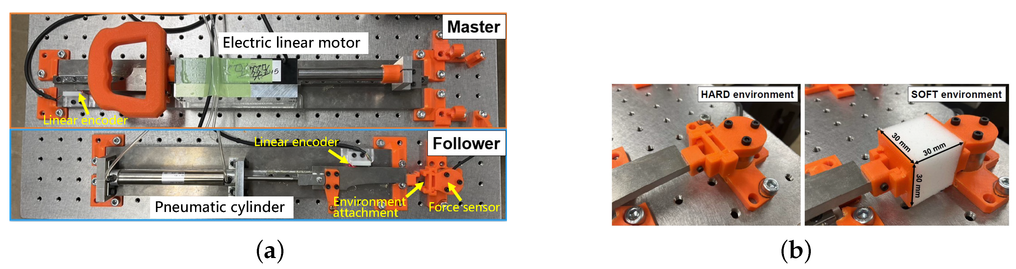
4.1. Hardware Configuration

The experimental system used in this study is the same as that in our previous study [24], and its configuration is shown in Figure 6a. A frictionless linear shaft motor is used for the leader. A pneumatic cylinder is used for the follower, and its driving force is controlled using differential pressure at the output port of a five-port servo valve. A force sensor is installed on the follower side to measure the environmental reaction force, which was used to evaluate the experimental results. The control period is 1 kHz. The specifications of the main components of the experimental system are shown in

Table 3. Specifications of main components of the leader–follower experimental system.

Leader	Linear motor	Maker	GMC Hillstone Co., Ltd., Yamagata, Japan
		Model	s160Q
		Stroke	100 mm
		Rated thrust	20 N
		Mass of moving part	0.676 kg
	Linear encoder	Maker	Technohands Co., Ltd., Kanagawa, Japan
		Model	TAi-200
		Position resolution	1.0 $\mathsf{\mu }$m
Follower	Air cylinder	Maker	SMC Corp., Tokyo, Japan
		Model	CJ2XE16-100Z
		Bore	$\varphi$ 16 mm
		Stroke	100 mm
		Actuation type	Double acting
		Mass of moving part	0.125 kg
	Linear encoder	Maker	Technohands Co., Ltd., Kanagawa, Japan
		Model	TAi-200
		Position resolution	1.0 $\mathsf{\mu }$m

. In addition, two types of materials (HARD/SOFT) are prepared as the contact environment of the experiment, as shown in Figure 6b. The HARD environment is made of ABS, and the SOFT environment is made of melamine sponge.

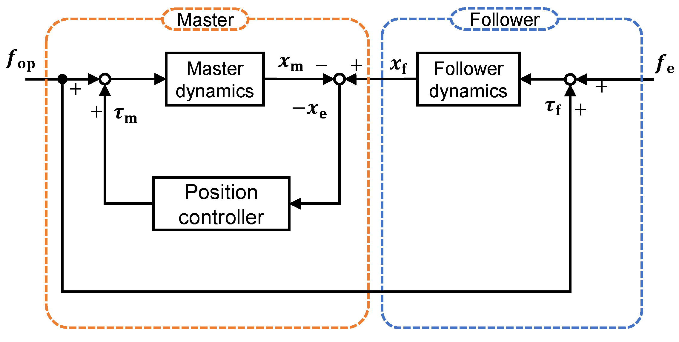
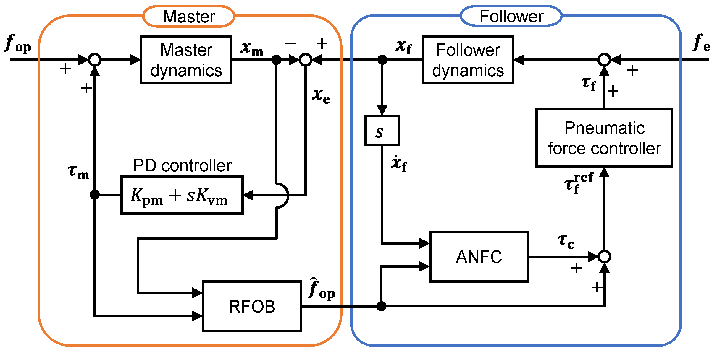
4.2. Design of the Bilateral Control System

In this experiment, the proposed ANFC was implemented in the force-projecting type. A block diagram of the control system is shown in Figure 7. The operational force $f_{\mathrm{op}}$ is estimated at the leader side using a reaction force observer (RFOB) and sent to the follower. The leader receives the follower position as a reference value and is position-controlled by the PD controller. The follower is driven by the ANFC compensation term ${\tau }_{\mathrm{c}}$ added to the leader operational force $f_{\mathrm{op}}$.

Table 4. Position control parameters of the leader.

Description	Symbol	Value	Unit
Leader position gain	$K_{\mathrm{pm}}$	20.0	[N/mm]
Leader velocity gain	$K_{\mathrm{vm}}$	$2\sqrt{M_{\mathrm{m}}{K}_{\mathrm{pm}}}$	[Ns/mm]
Mass of the leader	$M_{\mathrm{m}}$	0.676	[kg]

describes the parameters of the leader position controller. The leader position gain $K_{\mathrm{pm}}$ was set through trial and error. The leader velocity gain $K_{\mathrm{vm}}$ was set to $K_{\mathrm{vm}}=2\sqrt{M_{\mathrm{m}}{K}_{\mathrm{pm}}}$ so that the system was critically damped.

Note that removing the ANFC term ${\tau }_{\mathrm{c}}$ from Figure 7 results in a simple force-projecting type. In the experiments described below, the control performances with and without the ANFC are compared.

5. Bilateral Control Experiment

We conducted the bilateral control experiment using the experimental system and control system described in Section 4 and compared the performance of the control system shown in Figure 7 with and without ANFC. Experiments were conducted on three items: operational performance in n- load condition, control response in contact with environment, and frequency response.

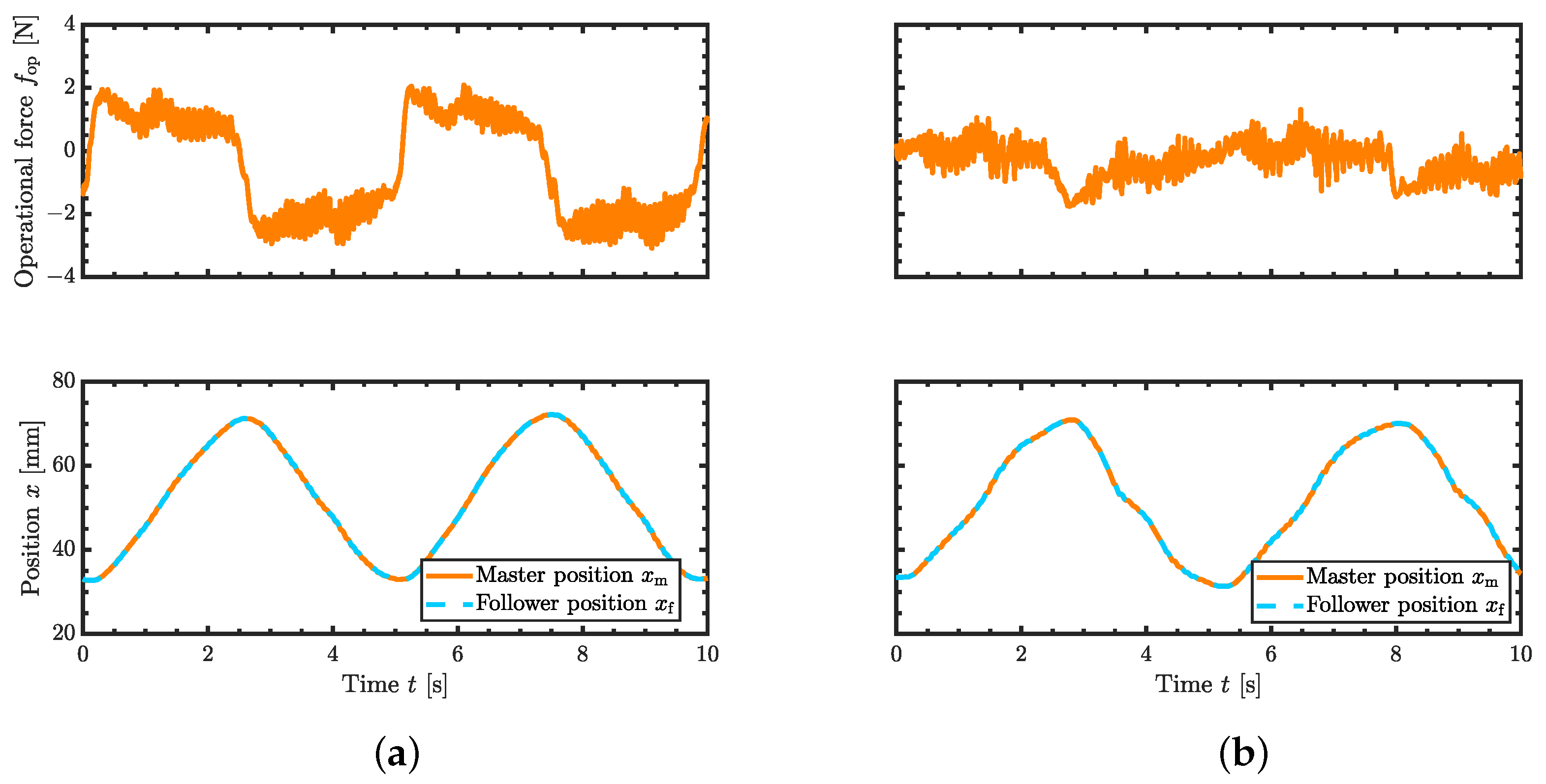
5.1. Operational Performance in No-Load Condition

To investigate the heaviness of the operational force during free movement, an operational performance experiment in the no-load condition was conducted. During free movement, the system should be able to move lightly without being affected by the follower dynamics. In the experiment, the leader was manually operated to reciprocate back and forth with no obstacles on the follower side. The leader operational force and position responses in this experiment are shown in Figure 8. The normal force-projecting type without ANFC requires an operational force of approximately 2 to −3 N. In contrast, that with ANFC requires about 1 to −1.5 N, demonstrating a significant reduction in the operational force. The reason for the slightly asymmetric operational force between the forward and return strokes was the compensation error of the cogging force in the leader’s RFOB. Regarding the position control response, both systems demonstrated good tracking performance. This indicates that they retained the advantage of the force-projecting type in overcoming the low positioning stiffness of the pneumatic follower.

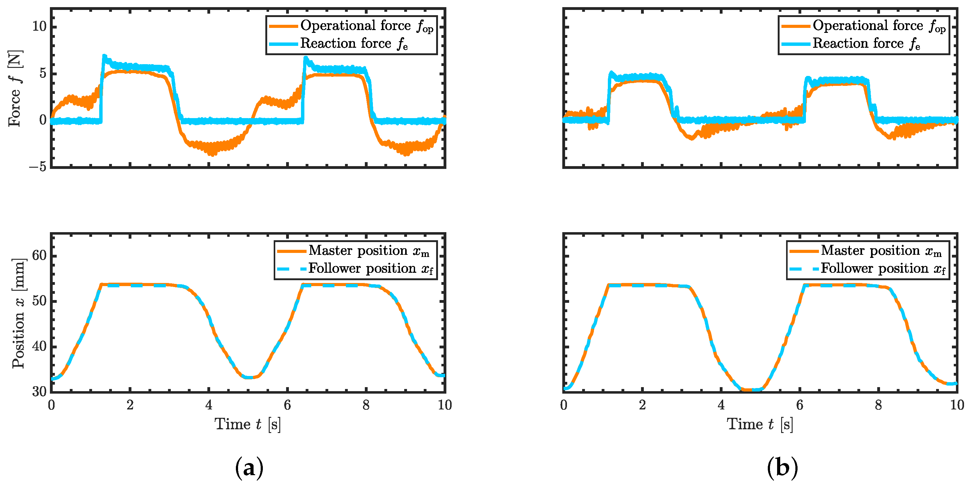
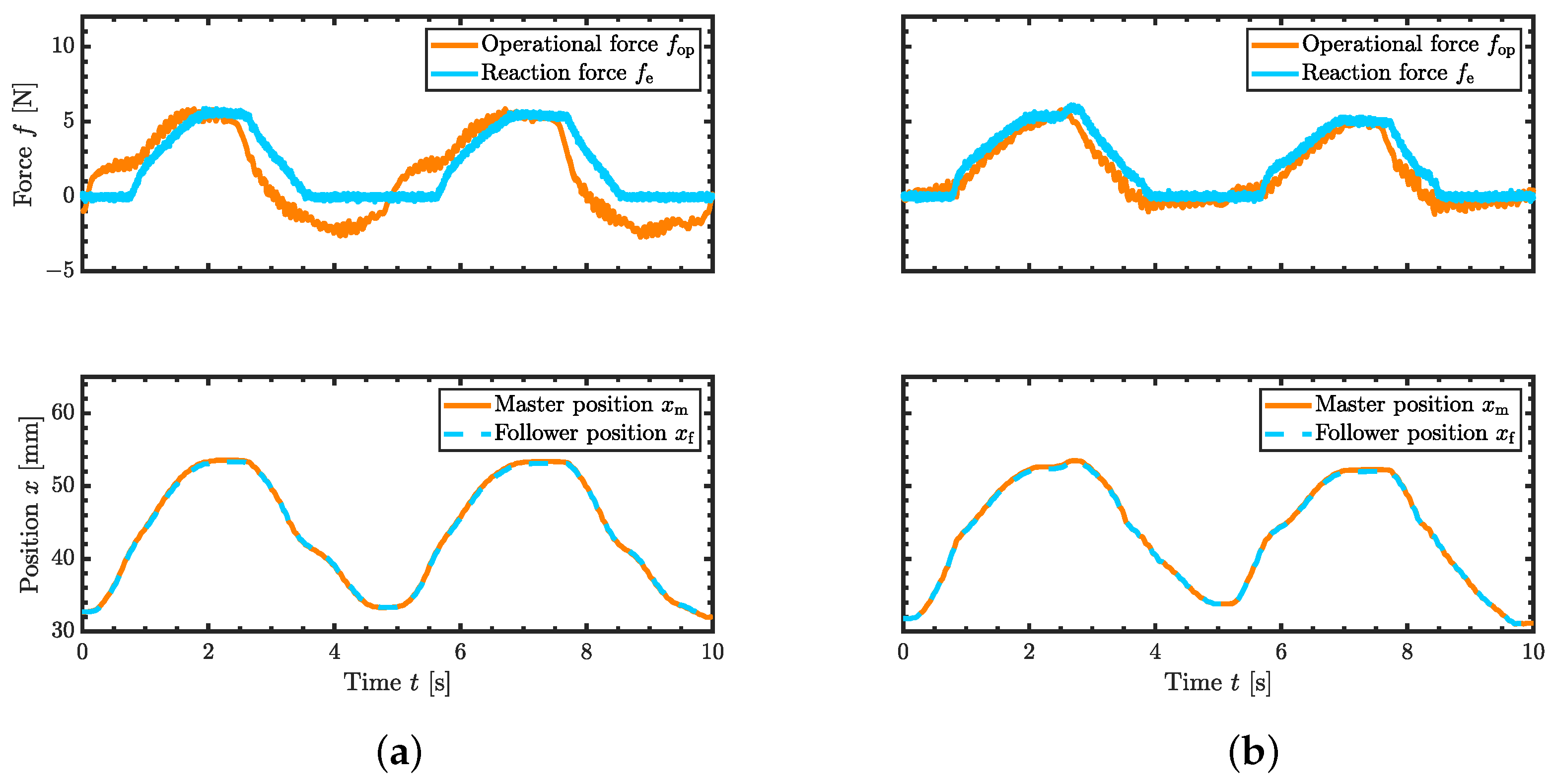
5.2. Control Response in Contact with Environment

Experiments were conducted to bring the follower into contact with each “HARD” and “SOFT” environment shown in Figure 6b by manually operating the leader. According to the principle of transparency of bilateral control, the force exerted by the follower on the environment should match the leader’s operational force. The experimenter started at a distance of about 35 mm between the follower and the environment, pushed the follower into the environment with an operational force of about 5 N, and then returned it to its original position. This series of contact manipulations was performed 6 times within 35 s. Transient responses lasting 10 s were extracted as time histories from each sequence of contact tasks, and the results are presented below.

First, the bilateral control responses when in contact with the HARD environment are shown in Figure 9. When the follower is stationary and in contact with the wall, which is made of hard plastic, the influence of dynamics is eliminated. As a result, the operational and environmental reaction forces are well matched, regardless of the presence or absence of the ANFC. However, when the ANFC is applied, the force sensed by the operator during a collision with the wall is considered to be better reproduced because the operational force during free movement is lighter with the ANFC as shown in Section 5.1. With the ANFC, at the moment when the operational force pressed against the wall is released (around 3 s and 8 s), the follower reaction force makes an unexpected slight change due to the switching of the friction compensation force. Even with smoothing of the compensation force switching, this behavior is likely to occur in situations where the force and velocity change abruptly, as in this case.

Second, the bilateral control responses when in contact with the SOFT environment are shown in Figure 10. Since the environmental material is an elastic sponge, the follower is allowed to move in contact with it under a reaction force. Therefore, the application effect of the ANFC is well obtained, which results in a clear improvement of consistency between the operational force and the environmental reaction force.

To quantitatively evaluate performance, the root mean square error (RMSE), normalized root mean square error (NRMSE = RMSE/$f_{\mathrm{op}\max }$), standard deviation of errors, and maximum error were calculated for the force error $f_{\mathrm{op}}-f_{\mathrm{e}}$ and position error $x_{\mathrm{m}}-x_{\mathrm{f}}$ throughout the whole experimental process. The values are presented in

Table 5. Parameters of force and position error in HARD environment.

		Without ANFC	With ANFC
Force	RMSE [N]	1.81	0.83
	NRMSE	0.25	0.16
	Standard deviation [N]	1.73	0.71
	Max error [N]	3.92	2.41
Position	RMSE [mm]	0.17	0.13
	NRMSE	0.022	0.025
	Standard deviation [mm]	0.16	0.12
	Max error [mm]	0.37	0.26

and

Table 6. Parameters of force and position error in SOFT environment.

		Without ANFC	With ANFC
Force	RMSE [N]	1.62	0.73
	NRMSE	0.21	0.13
	Standard deviation [N]	1.53	0.55
	Max error [N]	2.84	1.28
Position	RMSE [mm]	0.18	0.13
	NRMSE	0.023	0.022
	Standard deviation [mm]	0.16	0.10
	Max error [mm]	0.38	0.29

for each of the two types of environments. Focusing first on the force error, it can be confirmed that the error was significantly reduced in both the HARD environment and the SOFT environment when applying the proposed ANFC. When comparing NRMSE, an improvement of approximately 36% was achieved in the HARD environment, reducing from 0.25 to 0.16, and an improvement of approximately 38% was achieved in the SOFT environment, reducing from 0.21 to 0.13. The force error variations, as expressed in the standard deviations, were also dramatically reduced by applying the ANFC. It should be noted that the follower was almost stationary at the moment of contact with the HARD environment, which caused the nonlinearities of the dynamics to become more pronounced. As a result, the maximum force error was considered to be larger compared to the SOFT environment. Focusing next on the position error data, it can also be said that positioning performance was improved when applying the ANFC. This improvement was due to the compensation force provided by the ANFC, which lightened the operational feel and reduced the operational force load on the position control at the leader side.

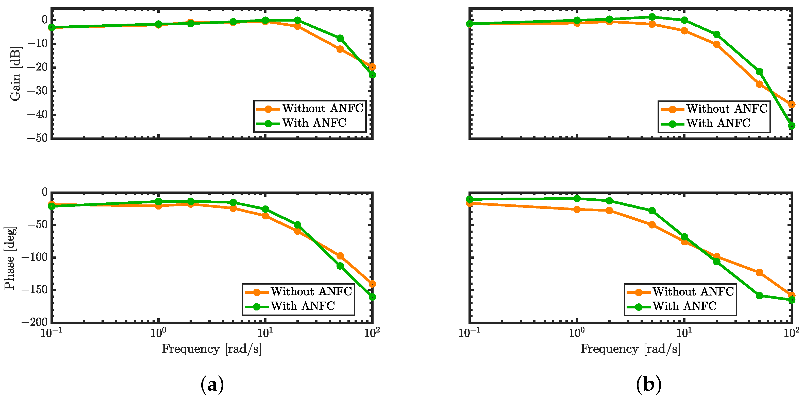
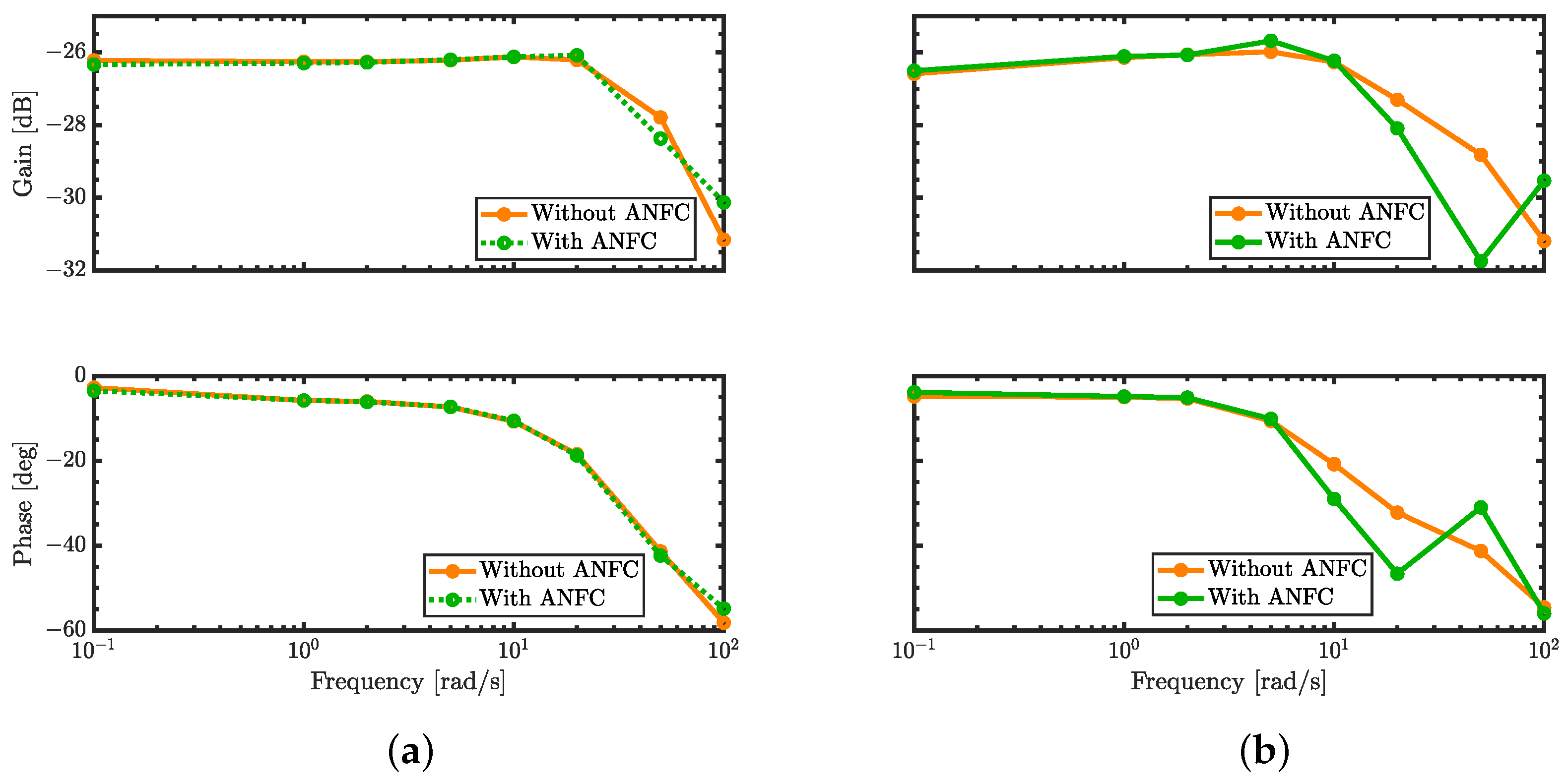
5.3. Frequency Response

To clarify the dynamic characteristics of the experimental bilateral control system with the ANFC, the system was assumed to be linearly approximated. Under this assumption, the frequency responses of the transfer functions $G_{\mathrm{f}}$ and $G_{\mathrm{x}}$, defined by the following equation, were investigated in the experiment.

$$\begin{array}{ccc}\hfill G_{\mathrm{f}}& =& -{\displaystyle \frac{\mathcal{L}\left[f_{\mathrm{e}}\right]}{\mathcal{L}\left[f_{\mathrm{op}}\right]}}\hfill \end{array}$$

(20)

$$\begin{array}{ccc}\hfill G_{\mathrm{x}}& =& {\displaystyle \frac{\mathcal{L}[x_{\mathrm{m}}-x_{\mathrm{f}}]}{\mathcal{L}\left[f_{\mathrm{op}}\right]}}\hfill \end{array}$$

(21)

Both transfer functions take the leader operational force as input. $G_{\mathrm{f}}$ and $G_{\mathrm{x}}$ represent the dynamic characteristics of the follower environmental reaction force and the position error between the leader and follower, respectively. The follower is fixed in an environment, HARD or SOFT. The driving force of the leader is generated and input to the experimental system so that the operational force is the following sine wave:

$$\begin{array}{c}\hfill f_{\mathrm{op}}=5sin\left(\omega t\right)\end{array}$$

(22)

The angular frequency $\omega$ was given eight points: 0.1, 1, 2, 5, 10, 20, 50, and 100 rad/s.

The frequency responses of $G_{\mathrm{f}}$ and $G_{\mathrm{x}}$ obtained in this experiment are shown in the Bode diagrams. Figure 11 shows the frequency responses of $G_{\mathrm{f}}$, while Figure 12 shows that of $G_{\mathrm{x}}$.

First, the results of the force transfer function $G_{\mathrm{f}}$ are described. Ideally, its gain should be zero because the operational force and environmental reaction force should be equal in magnitude, as shown in Equation (7). In Figure 11a, since the follower is quasi-static, constrained by a hard wall, generally similar characteristics were obtained with and without the ANFC. However, a slight difference was observed around 20 rad/s, suggesting that the effect of the ANFC functions predominantly. In the response of $G_{\mathrm{f}}$ in the SOFT environment shown in Figure 11b, since the follower was able to move under the environmental reaction force, the effect of property improvement by the ANFC was more pronounced. Note that no force resonance was observed in both environments.

Second, the results of the transfer function of the position error $G_{\mathrm{x}}$ are described. Since a small position error is desirable, its gain should also be small. Figure 12a,b show that in both environments, the gain value is kept below approximately −26 dB. These are good results in which the positioning stiffness of the electric leader functioned effectively, as in the experiments in our previous study [24].

6. Discussion

The experimental results demonstrated that the proposed ANFC reduces the heaviness of the operation feeling. It also improved the force reproducibility (the consistency between the leader operational force and the follower environmental reaction force) of the force-projecting type for the pneumatic follower. The ANFC algorithm, which switches the parameters of the compensating force calculation depending on the magnitude of the operational force and the motion state, ensures good force reproducibility, regardless of whether the manipulator is unloaded/loaded and in motion/at rest.

The ANFC is particularly useful for systems in which the control stiffness and responsiveness of the leader and follower differ greatly, and external forces on the follower side cannot be accurately measured, which is the target of this study. In recent studies, an adaptive coordinated controller has been proposed to enhance transient stability and voltage regulation performance in power systems under unknown generator parameters [42]. The controller is a regulator-type control system with a fixed setpoint and requires an uncertain state feedback structure. Unlike this type of controller, a significant advantage of ANFC is that performance can be improved only through feedforward compensation without implementing a force feedback loop, thereby facilitating system stability. The second advantage is that the excellent position control characteristics of the electric leader can be maximized by maintaining a simple two-channel control structure. However, the effect of switching the compensation parameters may cause unnatural changes in the follower driving force with the ANFC. One approach to mitigate this effect is introducing a more precise nonlinear friction model such as the LuGre friction model [39]. Another approach is to utilize deep learning techniques, such as LSTM, for identifying the nonlinear dynamics of the follower. Compared to physics-based modeling approaches, the data-driven approach using neural networks is expected to provide high expressiveness for nonlinear components. Furthermore, recent studies have demonstrated that deep reinforcement learning is effective for tuning nonlinear control systems [43]. For further improving the performance of the ANFC, deep reinforcement learning techniques can be utilized to derive the optimal smoothing function and tune the control parameters.

7. Conclusions

In this study, a method of adaptive nonlinear friction compensation (ANFC) was developed to improve the performance of force-projecting type bilateral control applied to a pneumatic follower. The proposed method compensates the follower’s driving force by adaptively switching between two types of friction compensation forces calculated from the admittance target velocity derived from the leader’s operating force and the follower’s current velocity, depending on the dynamic state of the system. Experiments using a 1-DOF bilateral teleoperation system demonstrated that force reproducibility improved by 36% when contacting a HARD environment and by 38% when contacting a SOFT environment. In addition, frequency response tests confirmed improved dynamic characteristics and system stability. In future work, we will develop a method to apply ANFC to a multi-DOF manipulator and evaluate its control performance via experiments.

References

1. Tadano, K.; Kawashima, K. Development of a Master Slave Manipulator with Force Display Using Pneumatic Servo System for Laparoscopic Surgery. Int. J. Assist. Robot. Syst. 2007, 8, 6–13. [Google Scholar]
2. Tadano, K.; Kawashima, K. Development of a Master Slave System with Force Sensing Using Pneumatic Servo System for Laparoscopic Surgery. In Proceedings of the 2007 IEEE International Conference on Robotics and Automation, Rome, Italy, 10–14 April 2007; pp. 947–952. [Google Scholar]
3. Kanno, T.; Haraguchi, D.; Yamamoto, M.; Tadano, K.; Kawashima, K. A Forceps Manipulator with Flexible 4-DOF Mechanism for Laparoscopic Surgery. IEEE/ASME Trans. Mechatron. 2015, 20, 1170–1178. [Google Scholar] [CrossRef]
4. Haraguchi, D.; Kanno, T.; Tadano, K.; Kawashima, K. A Pneumatically Driven Surgical Manipulator With a Flexible Distal Joint Capable of Force Sensing. IEEE/ASME Trans. Mechatron. 2015, 20, 2950–2961. [Google Scholar] [CrossRef]
5. Kawashima, K.; Sasaki, T.; Miyata, T.; Nakamura, N.; Sekiguchi, M.; Kagawa, T. Development of Robot Using Pneumatic Artificial Rubber Muscles to Operate Construction Machinery. J. Robot. Mechatron. 2004, 16, 8–16. [Google Scholar] [CrossRef]
6. Sasaki, T.; Kawashima, K. Remote control of backhoe at construction site with a pneumatic robot system. Autom. Constr. 2008, 17, 907–914. [Google Scholar] [CrossRef]
7. Anderson, R.J.; Spong, M.W. Bilateral control of teleoperators with time delay. In Proceedings of the 1988 IEEE International Conference on Systems, Man, and Cybernetics, Beijing, China, 8–12 August 1988; Volume 1, pp. 131–138. [Google Scholar]
8. Imaida, T.; Yokokohji, Y.; Doi, T.; Oda, M.; Yoshikawa, T. Ground–Space Bilateral Teleoperation of ETS-VII Robot Arm by Direct Bilateral Coupling Under 7-s Time Delay Condition. IEEE Trans. Robot. Autom. 2004, 20, 499–511. [Google Scholar] [CrossRef]
9. Kim, W.S.; Hannaford, B.; Fejczy, A.K. Force-reflection and shared compliant control in operating telemanipulators with time delay. IEEE Trans. Robot. Autom. 1992, 8, 176–185. [Google Scholar] [CrossRef]
10. Polushin, I.G.; Liu, P.X.; Lung, C.H. A Force-Reflection Algorithm for Improved Transparency in Bilateral Teleoperation With Communication Delay. IEEE/ASME Trans. Mechatron. 2007, 12, 361–374. [Google Scholar] [CrossRef]
11. Lee, D.; Spong, M.W. Passive Bilateral Teleoperation With Constant Time Delay. IEEE Trans. Robot. 2006, 22, 269–281. [Google Scholar] [CrossRef]
12. Kostyukova, O.; Vista, F.P.; Chong, K.T. Design of feedforward and feedback position control for passive bilateral teleoperation with delays. ISA Trans. 2019, 85, 200–213. [Google Scholar] [CrossRef]
13. Yokokohji, Y.; Hosotani, N.; Yoshikawa, T. Analysis of maneuverability and stability of micro-teleoperation systems. In Proceedings of the 1994 IEEE International Conference on Robotics and Automation, San Diego, CA, USA, 8–13 May 1994; Volume 1, pp. 237–243. [Google Scholar]
14. Yokokohji, Y.; Yoshikawa, T. Bilateral control of master-slave manipulators for ideal kinesthetic coupling-formulation and experiment. IEEE Trans. Robot. Autom. 1994, 10, 605–620. [Google Scholar] [CrossRef]
15. Komada, S.; Ohnishi, K. Control of robotic manipulators by joint acceleration controller. In Proceedings of the 15th Annual Conference of IEEE Industrial Electronics Society, Philadelphia, PA, USA, 6–10 November 1989; Volume 3, pp. 623–628. [Google Scholar]
16. Iida, W.; Ohnishi, K. Reproducibility and operationality in bilateral teleoperation. In Proceedings of the 8th IEEE International Workshop on Advanced Motion Control, 2004, AMC ’04, Kawasaki, Japan, 28 March 2004; pp. 217–222. [Google Scholar]
17. Katsura, S.; Matsumoto, Y.; Ohnishi, K. Modeling of Force Sensing and Validation of Disturbance Observer for Force Control. IEEE Trans. Ind. Electron. 2007, 54, 530–538. [Google Scholar] [CrossRef]
18. Murakami, T.; Yu, F.; Ohnishi, K. Torque sensorless control in multidegree-of-freedom manipulator. IEEE Trans. Ind. Electron. 1993, 40, 259–265. [Google Scholar] [CrossRef]
19. Chen, Z.; Huang, F.; Yang, C.; Yao, B. Adaptive Fuzzy Backstepping Control for Stable Nonlinear Bilateral Teleoperation Manipulators With Enhanced Transparency Performance. IEEE Trans. Ind. Electron. 2020, 67, 746–756. [Google Scholar] [CrossRef]
20. Chen, Z.; Huang, F.; Sun, W.; Gu, J.; Yao, B. RBF-Neural-Network-Based Adaptive Robust Control for Nonlinear Bilateral Teleoperation Manipulators With Uncertainty and Time Delay. IEEE/ASME Trans. Mechatron. 2020, 25, 906–918. [Google Scholar] [CrossRef]
21. Batty, T.; Ehrampoosh, A.; Shirinzadeh, B.; Zhong, Y.; Smith, J. A Transparent Teleoperated Robotic Surgical System with Predictive Haptic Feedback and Force Modelling. Sensors 2022, 22, 9770. [Google Scholar] [CrossRef]
22. Kikuuwe, R.; Kanaoka, K.; Kumon, T.; Yamamoto, M. Phase-Lead Stabilization of Force-Projecting Master-Slave Systems With a New Sliding Mode Filter. IEEE Trans. Control. Syst. Technol. 2015, 23, 2182–2194. [Google Scholar] [CrossRef]
23. Monden, R.; Kanno, T.; Haraguchi, D. Analytical Evaluation of Force-Projecting Bilateral Control for Pneumatic Manipulators. IFAC-PapersOnLine 2023, 56, 9998–10003. [Google Scholar] [CrossRef]
24. Haraguchi, D.; Monden, R. Fundamental Study on Force-Projecting Bilateral Control for Pneumatically Driven Follower Device. Actuators 2024, 13, 56. [Google Scholar] [CrossRef]
25. Haraguchi, D.; Monden, R. Teleoperation of Pneumatic Manipulators using Force-Projecting Bilateral Control. Dyn. Des. Conf. 2023, A33. [Google Scholar] [CrossRef]
26. Monden, Y.; Haraguchi, D. Sensorless Haptic Force Presentation using Force-Projecting Bilateral Control with Pneumatic Manipulator. In Proceedings of the 2024 IEEE 18th International Conference on Advanced Motion Control (AMC), Kyoto, Japan, 28 February–1 March 2024; pp. 1–6. [Google Scholar]
27. Chen, W.H.; Ballance, D.J.; Gawthrop, P.J.; O’Reilly, J. A nonlinear disturbance observer for robotic manipulators. IEEE Trans. Ind. Electron. 2000, 47, 932–938. [Google Scholar] [CrossRef]
28. Chen, W.H. Disturbance observer based control for nonlinear systems. IEEE/ASME Trans. Mechatron. 2004, 9, 706–710. [Google Scholar] [CrossRef]
29. Iwasaki, M.; Shibata, T.; Matsui, N. Disturbance-observer-based nonlinear friction compensation in table drive system. IEEE/ASME Trans. Mechatron. 1999, 4, 3–8. [Google Scholar] [CrossRef]
30. Wan, M.; Dai, J.; Zhang, W.H.; Xiao, Q.B.; Qin, X.B. Adaptive feed-forward friction compensation through developing an asymmetrical dynamic friction model. Mech. Mach. Theory 2022, 170, 104691. [Google Scholar] [CrossRef]
31. Zhang, W.; Li, M.; Gao, Y.; Chen, Y.Q. Periodic adaptive learning control of PMSM servo system with LuGre model-based friction compensation. Mech. Mach. Theory 2022, 167, 104561. [Google Scholar] [CrossRef]
32. Zhang, W.; Cao, B.; Nan, N.; Li, M.; Chen, Y.Q. An adaptive PID-type sliding mode learning compensation of torque ripple in PMSM position servo systems towards energy efficiency. ISA Trans. 2021, 110, 258–270. [Google Scholar] [CrossRef]
33. Dai, K.; Zhu, Z.; Shen, G.; Tang, Y.; Li, X.; Wang, W.; Wang, Q. Adaptive force tracking control of electrohydraulic systems with low load using the modified LuGre friction model. Control. Eng. Pract. 2022, 125, 105213. [Google Scholar] [CrossRef]
34. Zhang, B.; Wu, J.; Wang, L.; Yu, Z. Accurate dynamic modeling and control parameters design of an industrial hybrid spray-painting robot. Robot.Comput. Integr. Manuf. 2020, 63, 101923. [Google Scholar] [CrossRef]
35. Chen, Y.; Ding, J.; Chen, Y.; Yan, D. Nonlinear Robust Adaptive Control of Universal Manipulators Based on Desired Trajectory. Appl. Sci. 2024, 14, 2219. [Google Scholar] [CrossRef]
36. Li, A.; Qin, D. Adaptive model predictive control of dual clutch transmission shift based on dynamic friction coefficient estimation. Mech. Mach. Theory 2022, 173, 104804. [Google Scholar] [CrossRef]
37. Schindele, D.; Aschemann, H. Adaptive friction compensation based on the LuGre model for a pneumatic rodless cylinder. In Proceedings of the 2009 35th Annual Conference of IEEE Industrial Electronics, Porto, Portugal, 3–5 November 2009; pp. 1432–1437. [Google Scholar]
38. Liu, S.; Wang, L.; Wang, X.V. Sensorless force estimation for industrial robots using disturbance observer and neural learning of friction approximation. Robot. Comput. Integr. Manuf. 2021, 71, 102168. [Google Scholar] [CrossRef]
39. Xiao, J.; Dou, S.; Zhao, W.; Liu, H. Sensorless Human-Robot Collaborative Assembly Considering Load and Friction Compensation. IEEE Robot. Autom. Lett. 2021, 6, 5945–5952. [Google Scholar] [CrossRef]
40. Phuong, T.T.; Ohishi, K.; Yokokura, Y.; Miyasaki, T. Deep Learning Based Force-Sensor-Like Reaction Force Observer for Realization of Intelligent Force Sensing. In Proceedings of the 2024 IEEE 18th International Conference on Advanced Motion Control (AMC), Kyoto, Japan, 28 February–1 March 2024; pp. 1–6. [Google Scholar]
41. Lawrence, D.A. Stability and transparency in bilateral teleoperation. IEEE Trans. Robot. Autom. 1993, 9, 624–637. [Google Scholar] [CrossRef]
42. Fathollahi, A.; Andresen, B. Adaptive Fixed-Time Control Strategy of Generator Excitation and Thyristor-Controlled Series Capacitor in Multi-Machine Energy Systems. IEEE Access 2024, 12, 100316–100327. [Google Scholar] [CrossRef]
43. Gheisarnejad, M.; Fathollahi, A.; Sharifzadeh, M.; Laurendeau, E.; Al-Haddad, K. Data-Driven Switching Control Technique Based on Deep Reinforcement Learning for Packed E-Cell as Smart EV Charger. IEEE Trans. Transp. Electrif. 2025, 11, 3194–3203. [Google Scholar] [CrossRef]
Figure 1. Model of 1-DoF leader–follower system with sliding friction on the follower.
Actuators 14 00151 g001
Figure 2. Basic structure of force-projecting type.
Actuators 14 00151 g002
Figure 3. Block diagram of ANFC.
Actuators 14 00151 g003
Figure 4. Profile of mixing ratio γ .
Actuators 14 00151 g004
Figure 5. Flowchart showing the process by which the compensation force τ c is determined.
Actuators 14 00151 g005
Figure 6. Configuration of the experimental system [24]. (a) 1-DOF leader–follower system; (b) Two types of environmental walls connected by the follower cylinder rod.
Actuators 14 00151 g006
Figure 7. Block diagram of Force-projecting type with ANFC.
Actuators 14 00151 g007
Figure 8. Force and position responses in free movement: (a) with ANFC; (b) without ANFC.
Actuators 14 00151 g008
Figure 9. Bilateral control responses of force (upper) and position (lower) in contact with the HARD environment: (a) with ANFC; (b) without ANFC.
Actuators 14 00151 g009
Figure 10. Bilateral control responses of force (upper) and position (lower) in contact with the SOFT environment: (a) with ANFC; (b) without ANFC.
Actuators 14 00151 g010
Figure 11. Bode diagram of G f : (a) HARD environment; (b) SOFT environment.
Actuators 14 00151 g011
Figure 12. Bode diagram of G x : (a) HARD environment; (b) SOFT environment.
Actuators 14 00151 g012