Article

Comparative Study on Active Suspension Controllers with Parameter Adaptive and Static Output Feedback Control

Department of Mechanical and Automotive Engineering, Seoul National University of Science and Technology, Nowon-gu, Seoul 01811, Republic of Korea
Actuators 2025, 14(3), 150; https://doi.org/10.3390/act14030150
Submission received: 10 February 2025 / Revised: 11 March 2025 / Accepted: 17 March 2025 / Published: 18 March 2025
(This article belongs to the Special Issue Data-Driven Control for Vehicle Dynamics)

Abstract

:
This paper presents a comparative study on active suspension controllers for ride comfort. Two types of active suspension controllers are designed and compared in terms of ride comfort: static output feedback (SOF) and parameter adaptive ones, which have identical controller structure. A quarter-car model is selected as a vehicle model. To date, LQR has been used as an active suspension controller. LQR is hard to implement in real vehicles due to the full-state measurement requirement. To avoid the full-state measurement of LQR, SOF control is selected as a controller structure in this paper. Suspension stroke and its rate are selected as sensor outputs for SOF and parameter active controllers. Two types of SOF controllers are designed. The first is the LQ SOF controller, designed with the state-space model and LQ cost function. The second is SOF controllers, designed by simulation-based optimization (SBOM) for the quarter-car model with nonlinear spring and damper. A parameter adaptive controller is designed with the recursive lease square (RLS) algorithm and its equivalent extended Kalman filter (EKF). For comparison, LQR is designed and used as a baseline. From simulation results, it is shown that the static output feedback and parameter adaptive controllers are equivalent to each other in terms of controller structure and ride comfort and which conditions are needed for better control performance on those controllers.

1. Introduction

To date, it has been well known that there are two objectives in suspension control: ride comfort and road holding, which conflict with each other [1,2,3]. Generally, ride comfort is measured from the heave acceleration of a sprung mass (SPM), and road holding is measured from tire deflection. According to the frequency weightings representing sensitivity of the human body to vibration, specified in ISO2631-1:1997, the heave acceleration of the sprung mass within the range of 4–10 Hz is to be reduced for ride comfort improvement [4]. For this reason, it is necessary to reduce the heave acceleration of the SPM by a controller for ride comfort. In this paper, the control objective is to enhance ride comfort by reducing the heave acceleration of the SPM with a controller. For the purpose of enhancing ride comfort with a controller, various types of controllers have been applied [1,2,3,5,6,7]. Among various actuators such as active suspension, semi-active damper and air chamber, most of the approaches adopted active suspension as an actuator used to generate an active control force in a suspension. Several surveys on active suspension control can be found in [3,4,5,6,7,8].
Various controller design methodologies such as linear quadratic optimal control, H control, sliding mode control, backstepping control, fuzzy control, and adaptive control have been applied to design an active suspension controller [9,10,11,12,13,14]. Among these methodologies, the linear quadratic regulator (LQR) has been widely selected because it is systematic to design a controller for active suspension and easy to tune ride comfort and road holding [9].
To date, three typical vehicle models have been adopted when designing an active suspension controller: 2-DOF quarter-car, 4-DOF half-car and 7-DOF full-car ones [15,16,17]. Among them, the quarter-car model has been widely adopted for controller design. The quarter-car model can describe the vertical motions of the SPM and the unsprung mass (USPM). The half-car and full-car models can describe the vertical and pitch motions, and the vertical, pitch, and roll motions of the SPM, respectively. In this paper, the pitch and roll motions of the SPM are not considered because the control objective is to enhance ride comfort, which is measured with the vertical acceleration of the SPM. For the reason, a 2-DOF quarter-car model is used to design a controller for active suspension. From the model, a state-space model is derived. LQR is designed with the state-space model and LQ cost function, which is defined in such a way that the heave acceleration of the SPM is reduced by LQR [15,16].
LQR is a full-state feedback (FSF) controller, which requires all state variables to be measured by sensors or estimated by an observer. However, the state variables of the quarter-car model are hard to measure in real vehicles. To overcome this problem, an observer or state estimator has been applied [3]. However, a state observer requires exact values of model parameters, and this is hard to obtain in real vehicles [18]. In other words, performance of a state observer can be deteriorated by parameter uncertainties. To cope with this problem, SOF control is selected as a control structure instead of using an observer or a state estimator [14,15,16].
Figure 1 shows the schematic diagram of SOF and parameter adaptive controllers. In Figure 1, the suspension force, f, is generated by spring and damper forces, which are calculated by multiplying the spring stiffness, ks, and the damping coefficient, bs, by the suspension stroke and its rate, respectively. In the suspension, if the suspension force, f, acting between the SPM and USPM becomes zero, the heave acceleration of the SPM is not generated because there are no forces acting on the SPM. With this idea, the SOF controller (SOFC) and parameter adaptive controller (PAC) are designed in such a way that the suspension force between SPM and USPM becomes zero. For this reason, the suspension stroke and its rate are selected as a sensor output as given in Figure 1. As a result, SOFC and PAC have two gains, k1 and k2 in Figure 1, which correspond to spring stiffness, ks, and damping coefficient, bs, respectively. In this paper, the goal of controller design is to find these two gains. When designing controllers, it is assumed that non-ideal actuators with dead-zone and hysteresis nonlinearities are neglected in this paper [13].
In this paper, two types of SOFCs are designed: LQ SOF and SOF by SBOM as given in Figure 1. The first is the LQ SOF controller, designed with the LQ cost function [15,16]. This is designed with the state-space model of the quarter-car model. However, this method cannot be used if there are nonlinear elements in the model. The second is SOFC designed with the Simulink model and simulation-based optimization method (SBOM), SOF by SBOM in Figure 1 [19,20]. This is applied if the quarter-car model has nonlinear elements.
In this paper, a parameter adaptive controller (PAC) is designed with the suspension stroke and its rate, as shown in Figure 1 [13]. Identical to the previous SOFCs, the control objective of PAC is to make the suspension force be zero. More specifically, in Figure 1, the spring stiffness, ks, and damping coefficient, bs, are adaptively estimated by recursive least square (RLS) and its equivalent extended Kalman filter (EKF), which are depicted as the PAC with RLS and EKF as shown in Figure 1.
The goal of this paper is to design SOFC and PAC with the quarter-car model for ride comfort improvement and to compare those controllers in terms of controller structure and ride comfort. The contributions of this paper can be summarized as follows:
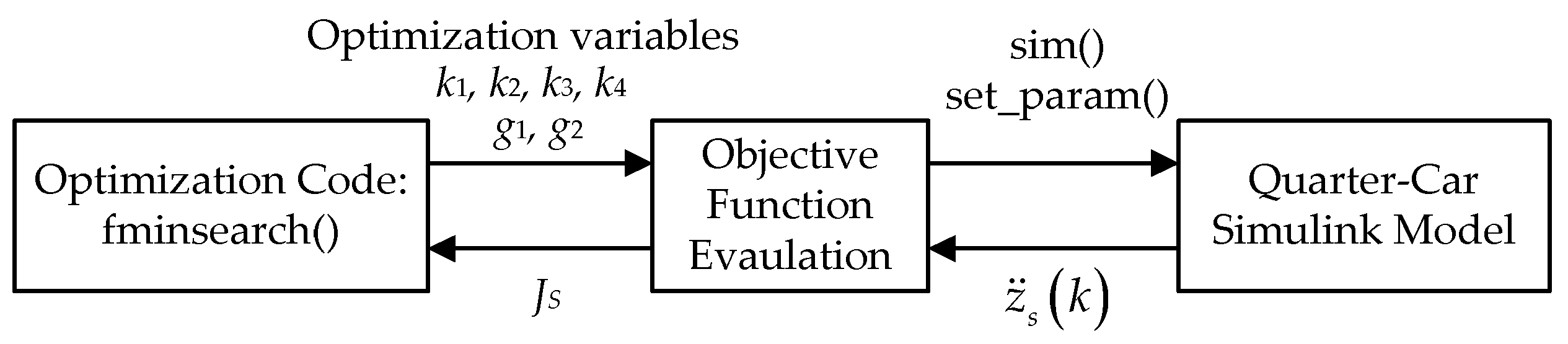
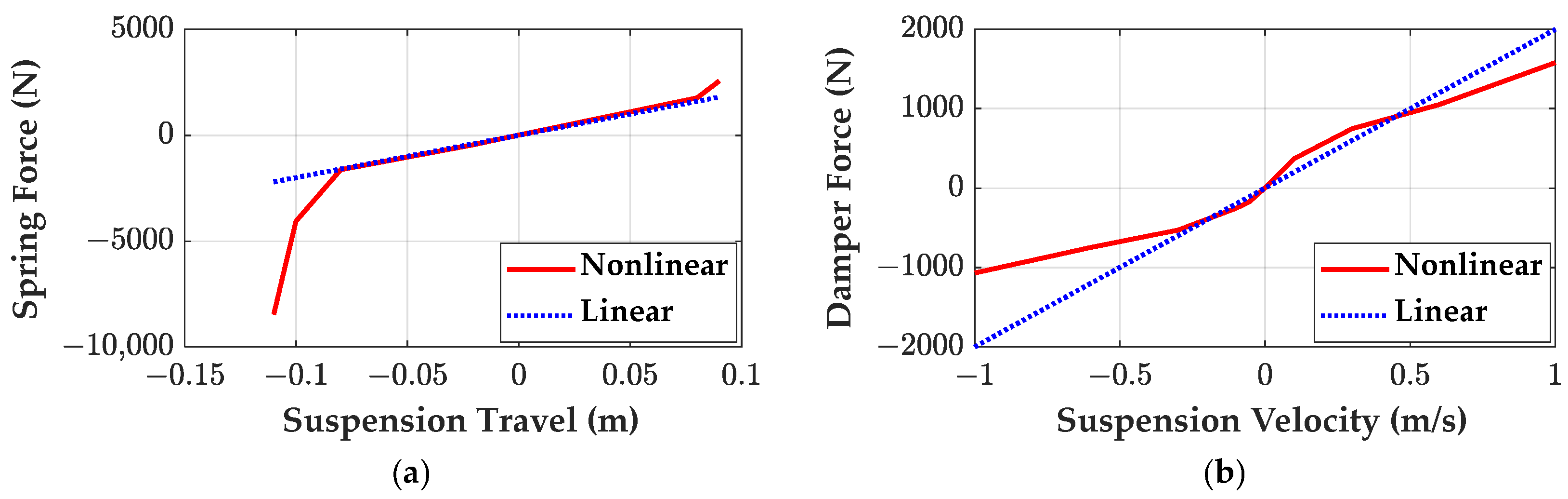
  • SOFC is designed by the LQ cost function and state-space model and by SBOM with the quarter-car model with nonlinear elements in order to reduce the heave acceleration of the SPM. These two types of SOFC are compared through simulation
  • PAC is designed by RLS and EKF in order to make the suspension force be zero.
  • By comparing the simulation results, it is shown that PAC is equivalent to or better than SOFCs. More specifically, the structures of SOFCs and PAC are identical to each other, and the performances of those controllers are equivalent to each other.
This paper is organized as follows: In Section 2, the 2-DOF quarter-car model is presented, and a state-space equation is derived from it. Based on the model, the active suspension controllers are design with LQR, LQ SOF control, and SBOM. In Section 3, simulation is conducted with the controllers. The conclusions are given in Section 4.

2. Design of Active Suspension Controllers
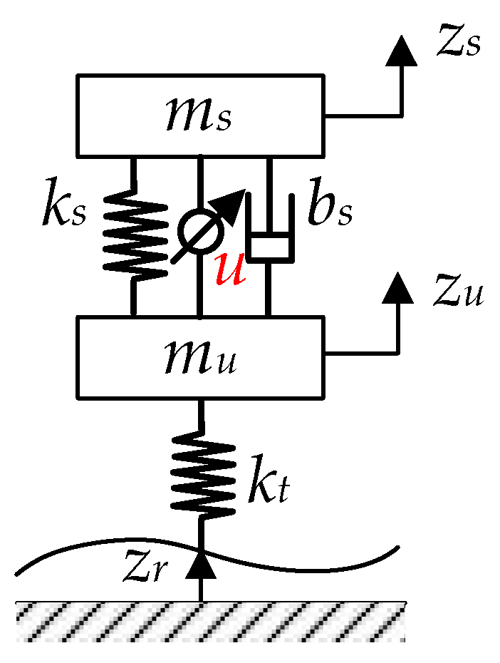
2.1. Vehicle Model

In this paper, a quarter-car model is selected as a vehicle one. Figure 2 shows the quarter-car model [15,16]. This model consists of the SPM and USPM, ms and mu, and spring and damper between them, which have the stiffness, ks, and the damping coefficient, bs, respectively. The vertical displacements of the SPM and UPSM are zs and zu, respectively. The control force, u, is applied to the SPM and USPM. The disturbance is the road profile or elevation, zr, which is applied to the UPSM with the stiffness of kt. The suspension force, f, applied between the SPM and USPM is given in (1). As shown in (1), the suspension force is generated for the spring and damper forces and the control input, u. In this paper, it is assumed that there are no suspension preloads or gravitational forces acting on the suspension. With the suspension force, (1), the equations of the motions of the SPM and USPM are given in (2). The state vector, x, is defined as (3). With (3), the state-space model of the quarter-car model is obtained as (4). In (4), the detailed derivation procedure of the system, disturbance, and input matrices, A, B1, and B2, can be found in the reference [15,16].
f = k s ( z s z u ) b s ( z ˙ s z ˙ u ) + u
m s z ¨ s = f m u z ¨ u = f k t z u z r
x z s z u z ˙ s z ˙ u T
x ˙ = A x + B 1 z r + B 2 u

2.2. Design of Static Output Feedback Controller

The LQ cost function, J, for active suspension control is defined as (5). Generally, the weights in J ρi have been set by Bryson’s rule, i.e., ρi = 1/ξi2, where ξi is the maximum allowable value (MAV) on the corresponding term [21]. For ride comfort improvement in J, ρ1 should be set to higher values while maintaining the others constant. Meanwhile, for road holding, ρ3 should be set to higher. ρ4 is used to limit the control effort.
J = 0 ρ 1 z ¨ s 2 + ρ 2 z s z u 2 + ρ 3 z u 2 + ρ 4 u 2 d t
A new vector, z, and matrices, C and D, are defined as (6). In (6), Ai,j is the element of A at the i-th row and j-th column, and B2,i is the element of B2 at the i-th row. With the vector and matrices defined in (6), (5) is represented as (7). LQR is a controller with the form of FSF, as given in (8), which minimizes J. In (8), the gain matrix, K, is easily calculated from the solution of the Riccati equation, P, for Q, N, and R. Let us denote this controller K as LQR.
z = C x + D u , C ρ 1 A 3 , 1 ρ 1 A 3 , 2 ρ 1 A 3 , 3 ρ 1 A 3 , 4 ρ 2 ρ 2 0 0 0 ρ 3 0 0 0 0 0 0 , D ρ 1 B 2 , 3 0 0 ρ 4
J = 0 z T z d t = 0 x u T Q N N T R x u d t , Q = C T C , N = C T D , R = D T D
u = K x = k 1 k 2 k 3 k 4 x = R 1 B 2 P
Generally, the state variables in x are hard to measure in real vehicles. There have been two methods to overcome this problem. The first is to use an estimator, and the second is to use an SOF control. In this paper, SOF control is adopted [15,16,17].
The SOF controller has the form of (9). As shown in (9), the control input, u, is calculated from not the state vector but the outputs. The vector of sensor outputs, y, is defined as (10) from the definition of the state vector, (3). As shown in (10), the suspension stroke and its rate are selected as a sensor output. With (10), the SOF controller of (9) can be represented as (11). As given in (11), the control input, u, has the form of (1), which is to be designed in such a way that the suspension force, f, becomes zero. If f is zero, it means that there are no forces acting on the SPM, resulting in no heave acceleration of the SPM. It has been known that it is impossible to analytically find the gain matrix of an SOF controller, G. For this reason, the optimization problem for the LQ SOF controller is formulated as (12) in order to find the optimum G that minimizes J. To solve (12), the meta-heuristic method, CMA-ES, is applied [15,16,17,19,20,22]. Let us denote this controller, G, as LQSOF.
u = G y
y = z s z u z ˙ s z ˙ u = 1 1 0 0 0 0 1 1 x = C x
u = g 1 g 2 z s z u z ˙ s z ˙ u = G y = G C x
min g 1 , g 2 J q = 1 2 trace P , P = P T > 0 s . t . max R e A + B 2 G C < 0 A + B 2 G C T P + P A + B 2 G C + Q + C T G T N T + N G C + C T G T R G C = 0
If there are nonlinear elements, spring and damper, in the quarter-car model, the state-space model cannot be derived. As a result, the LQR or LQSOF controller cannot be designed with the state-space model. To design a controller for the quarter-car model with nonlinear elements, simulation-based optimization (SBOM) is adopted [19,20].
The cost function of SBOM for ride comfort is given as (13). The optimization is performed by fminsearch(), a built-in function given in MATLAB 2019a. Figure 3 shows the procedure of SBOM [19,20]. In the case of SOFC, simulation is performed for a given g1 and g2 with the Simulink model of the quarter-car model for a simulation period. The disturbance used for simulation is a half-sine bump. From the simulation result, the cost function JS is calculated. Then, fminsearch() tries to find the optimum g1 and g2 that minimize JS. To guarantee the stability of the closed-loop system, the stability constraint, max(Re[A + B2GC]) < 0 as given in (12), is imposed. Let us denote this controller as SOFSBOM. This procedure of SBOM can be used to find the gains, k1, k2, k3, and k4 in K of LQR that minimize JS. Let us denote this controller as FSFSBOM.
J S = max k = 0 , 1 , , z ¨ s k

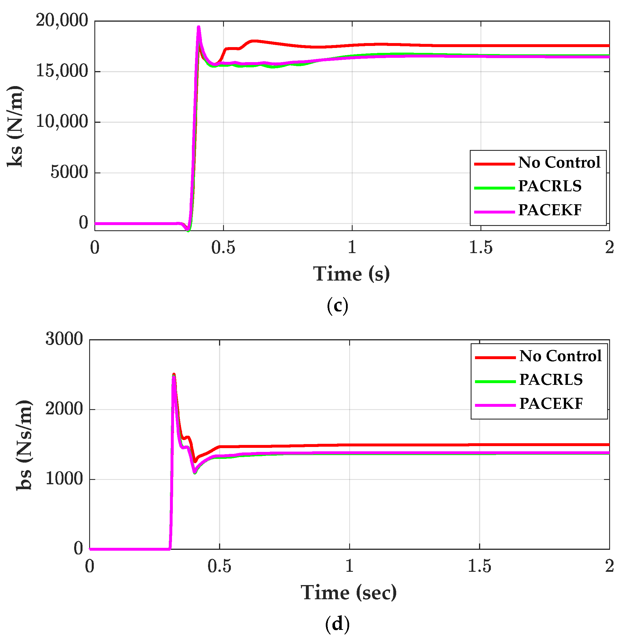
2.3. Design of Parameter Adaptive Controller

The parameter adaptive controller (PAC) originates from (1) and (2). In (1) and (2), if the suspension force, f, is zero, then it means that there are no forces acting on the sprung mass and that the disturbance acting on the sprung mass is perfectly canceled [13]. As a result, the heave acceleration of the sprung mass becomes zero, as given in (14). From (14), the control input, u, is obtained as (15). In (15), if the suspension stroke and its rate are measured by a sensor, then the parameters ks and bs can be estimated by a recursive least square (RLS). In fact, ks and bs act as the proportional and derivative gains, respectively. By comparing (15) with (11), it can be easily noticed that the structures of SOFC and PAC are identical to each other.
In the previous approach, the cubic terms of the suspension stroke and its rate were considered. As a result, four parameters were needed to calculate the control input, u [13]. Different from the approach, the cubic terms are not included into the control input, as shown in (15). This means that the spring and damper forces are linear with respect to the suspension stroke and its rate, respectively.
f = k s ( z s z u ) b s ( z ˙ s z ˙ u ) + u = m s z ¨ s = 0
u = k s z s z u + b s z ˙ s z ˙ u = z s z u z ˙ s z ˙ u k s b s
To derive RLS, the parameters and variables in (15) are represented in the form of the discrete-time ones. Two new vectors of the measurements and parameters, φ and θ, are defined as (16), respectively. With those vectors, (15) is represented as (17). The procedure of RLS is given in (18), (19), and (20). In (19), λ is the forgetting factor. Let us denote this controller as PACRLS.
φ k z s k z u k z ˙ s k z ˙ u k , θ k k s k b s k
u k = φ T k θ k
e k = m s z ¨ s k φ T k θ ^ k
H k + 1 = H k I φ k + 1 φ T k + 1 H k λ + φ T k + 1 H k φ k + 1
θ ^ k + 1 = θ ^ k + H k + 1 φ k + 1 e k + 1
Generally, RLS can be represented as an extended Kalman filter (EKF) [23,24,25,26]. With the vectors of φ and θ defined in (16), the new vectors are defined as (21). With those vectors, (15) is represented as the stochastic system, (22). In (22), μ and η are the white-noise processes of the system and measurement, respectively. M and N are the covariance matrices of system and measure noises, respectively. The time and measurement updates of EKF are given in (23) and (24), respectively. Different from RLS, there are two tuning parameters, M and N, in EKF. By virtue of this fact, the performance of EKF can be finely tuned by the elements of M and N. Let us denote this controller as PACEKF.
x p k θ ^ k , C p φ T k
x p k + 1 = x p k + μ k y p k = m s z ¨ s k = C p x p k + η k Μ k = E μ k μ T k , Ν k = E η k η T k
x ^ p k = x ^ p k 1 T ¯ k = M k + T k 1
K e = T ¯ k C p T Ν k + C p T ¯ k C p T x ^ p k = x ^ p k + Κ e y p k C p x ^ p k T k = I K e C p T ¯ k
The difference between the SOF controller and PAC is that the former has constant gain while the latter updates the parameters bs and ks in every time step. In view of computation amount, the SOF controller is preferred to PAC.
As given in (11), the SOF controller has two multiplications and one additional operation in a single iteration. This is quite simple to be run in a microprocessor. On the other hand, the computational complexity of RLS has been known as O(N2), where N is the number of coefficients [27]. As shown in (16), the number of coefficients in PACRLS is 2. Moreover, EKF given in (23) and (24) is equivalent to RLS. For this reason, PACRLS and PACEKF can be run in a microprocessor with little computational burden.
In real vehicles, the SOF controllers and PAC can be easily implemented on a microprocessor because the structure of those controllers is simple, and RLS and EKF have small dimensions. Moreover, the sensors such as an accelerometer and potentiometer/encoder for vertical acceleration and suspension stroke measurement have been available in real vehicles.

3. Simulation and Discussion

In this section, the designed controllers, LQSOF, FSFSBOM, SOFBOM, PACRLS, and PACEKF, are simulated. LQR is used as a baseline. From simulation results, the performance of the controllers is compared among one another in terms of ride comfort.

3.1. Simulation Environment

The parameters of the quarter-car model are given in Table 1. The weights in the LQ cost function are given in Table 2. As given in Table 2, the MAV on the heave acceleration of SPM, η1, is set to lower for ride comfort. When applying SBOM, the gain elements were bounded between −100,000 and 100,000. In SBOM, two road profiles were used as a disturbance. The first is the half-sine bump with the height of 0.05 m and the wavelength of 4 m, and the second is the sine waved road that has the wavelength and the amplitude of 12.2 m and 0.05 m. Let these two road profiles be called HSB and SWR, respectively. The vehicle speeds were set to 20 m/s and 10 m/s for the half-sine bump and the sine-waved road, respectively. As a result, there are four controllers designed by SBOM: FSFSBOM.HSB, SOFSBOM.HSB, FSFSBOM.SWR, and SOFSBOM.SWR. These controllers are compared with LQR and LQSOF in simulation. In SBOM, the actuator was modeled as the first-order system with a particular time-constant, which represents a bandwidth. The bandwidth of the actuator was set to 100 Hz. The sampling periods of PACRLS and PACEKF were set to 1 ms. The effects of the actuator bandwidth on the performance will be discussed later. The simulation periods were set to 2 s and 5 s for HSB and SWR, respectively.
When applying SBOM with the Simulink model, the spring and damper curves of the nonlinear spring and damper were used as shown in Figure 4 [28]. In Figure 4, the dotted blue lines represent the linear spring and damper, calculated from the values in Table 1.
Table 3 shows the gain matrices of LQR, LQSOF, FSFSBOM, and SOFSBOM. In the case of the controllers designed by SBOM, HSB and SWR stand for half-sine bump and sine-waved road, respectively. In Table 3, three SOF controllers, i.e., LQSOF, SOFSBOM.HSB, and SOFSBOM.SWR, have similar gains. For example, the first elements of those controllers are similar to one another. This means that SBOM tries to find the gains which make (14) satisfied because the cost function JS is selected. From this fact, it is expected that PACRLS or PACEKF acts as SOFSBOM. On the contrary, the gain elements of LQR, FSFSBOM.HSB, and FSFSBOM.SWR are different from one another.

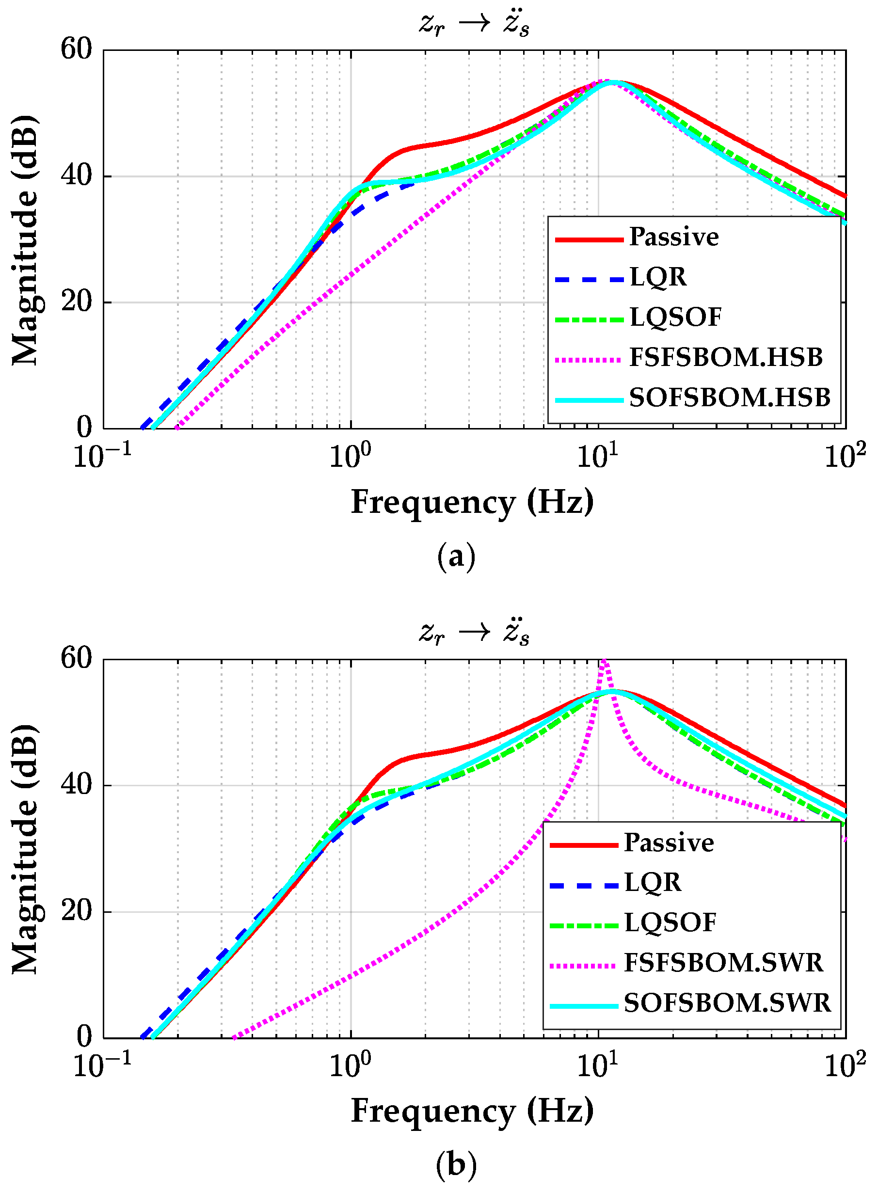
3.2. Frequency Response Analysis with the Designed Controllers

In this subsection, frequency response analysis is performed on the controllers given in Table 3. Figure 5 shows the frequency responses of the SOF controllers designed on HSB and SWR, drawn with the state-space model of (4). As shown in Figure 5, LQSOF and SOFSBOM are equivalent to one another in terms of ride comfort. In other words, those three controllers reduced the heave acceleration of the SPM over the range from 4 to 10 Hz, as provided in ISO2631-1:1997. FSFSBOM outperforms the other controllers. However, FSFSBOM.SWR shows an abnormal peak near 10 Hz, i.e., the resonance frequency of the USPM. This can have negative effects on the durability of the suspension. From those results, it is expected that the SOF controllers can provide good performance and that FSFSBOM shows the best performance in terms of ride comfort.

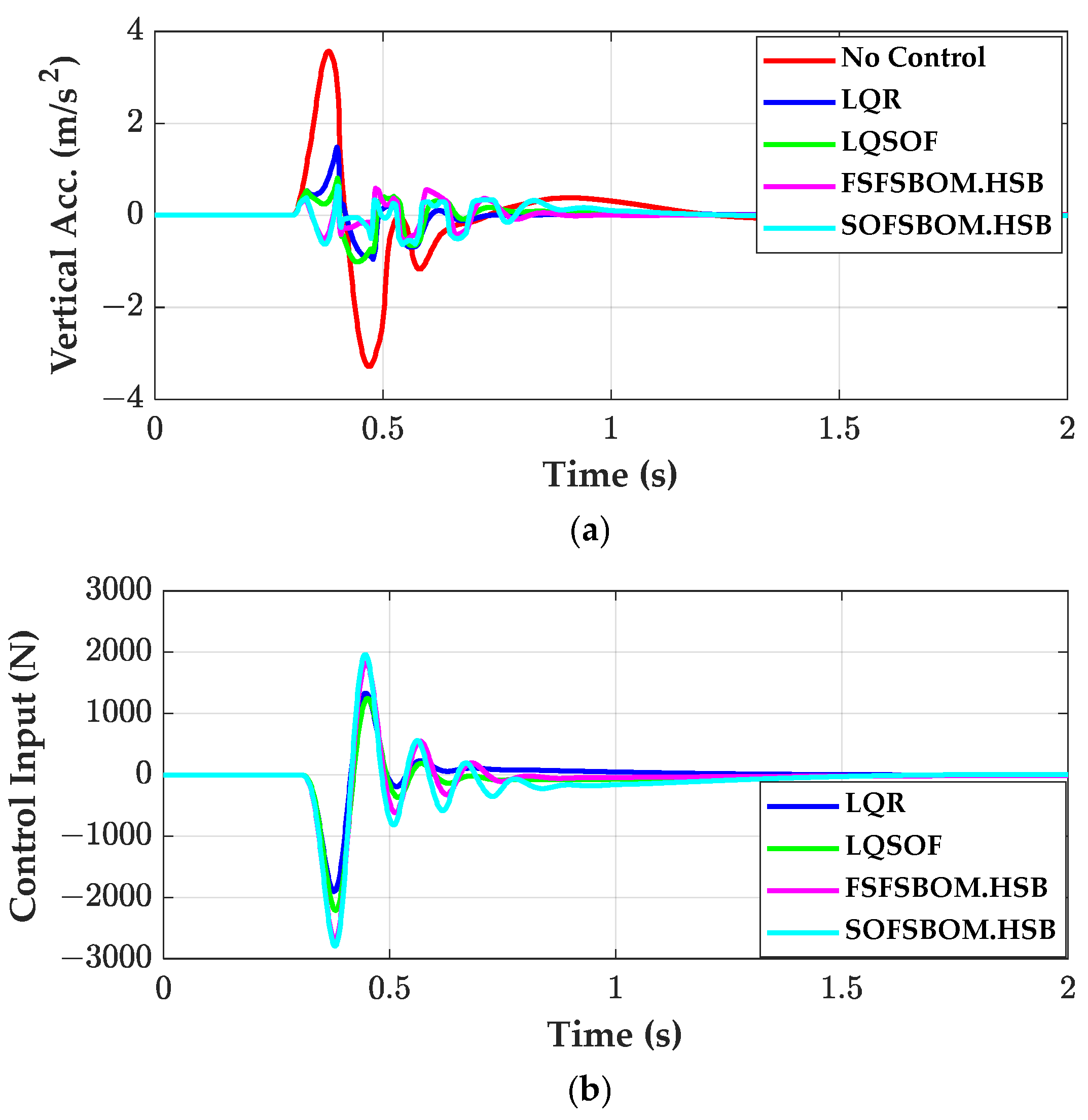
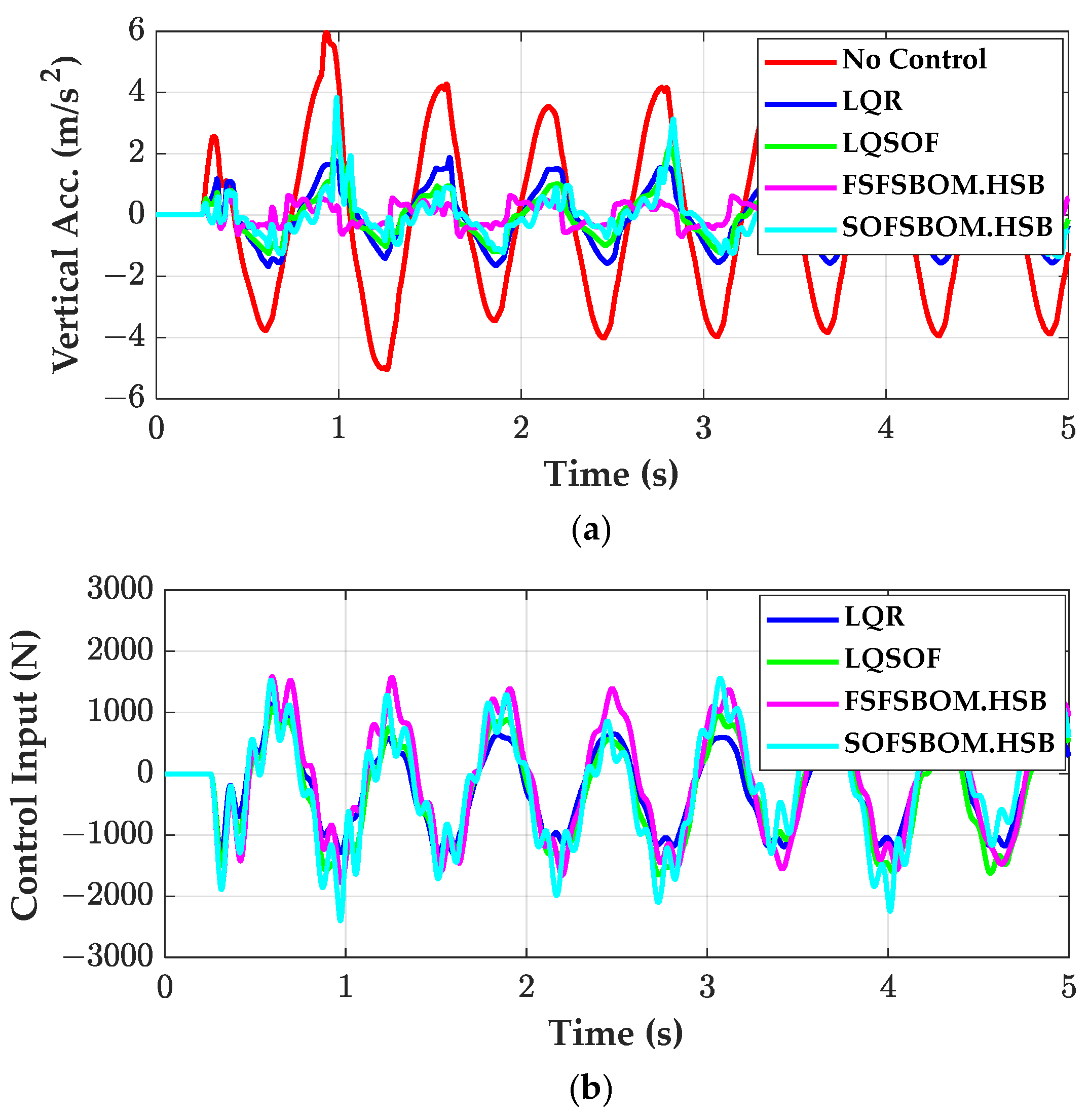
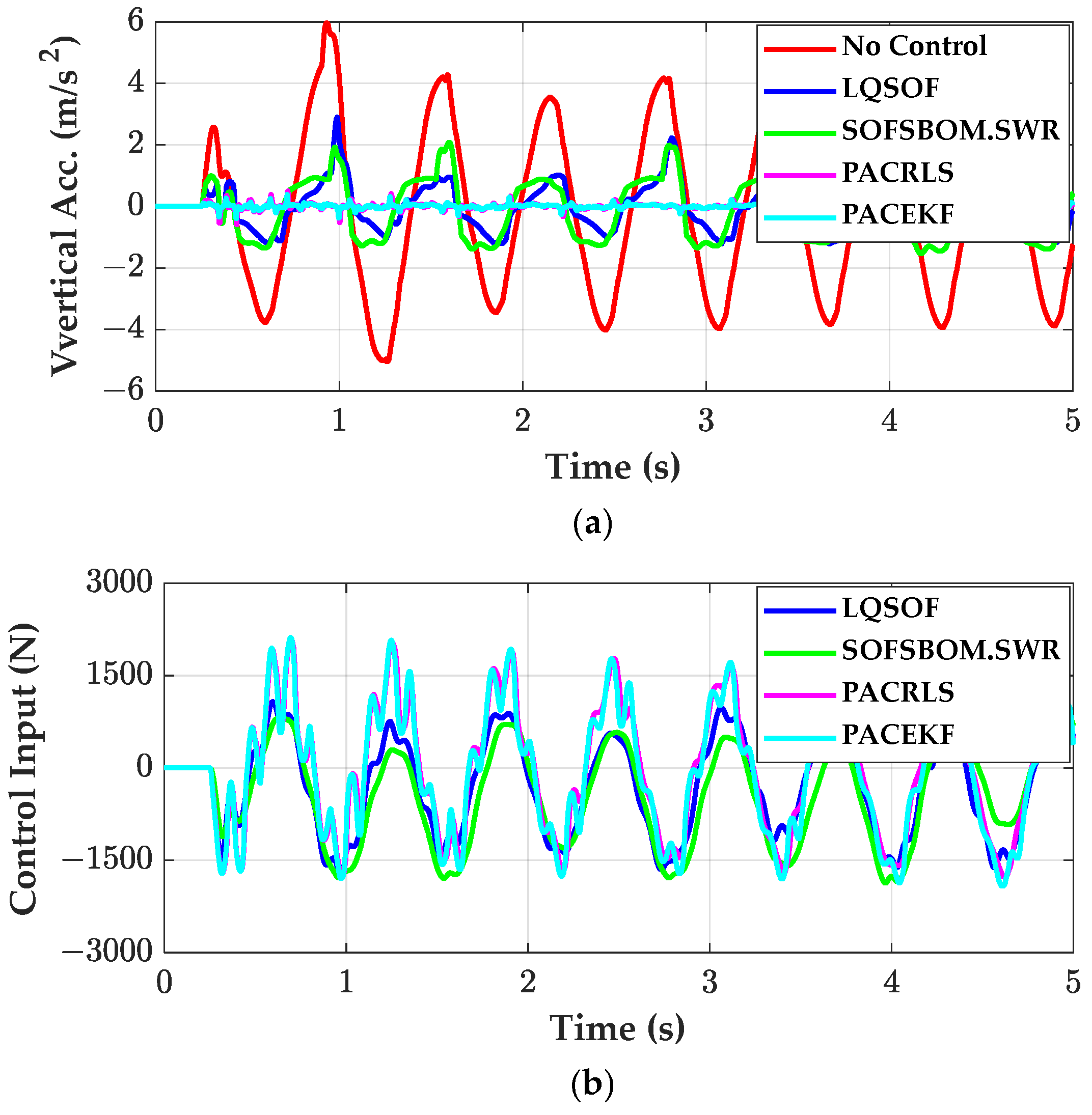
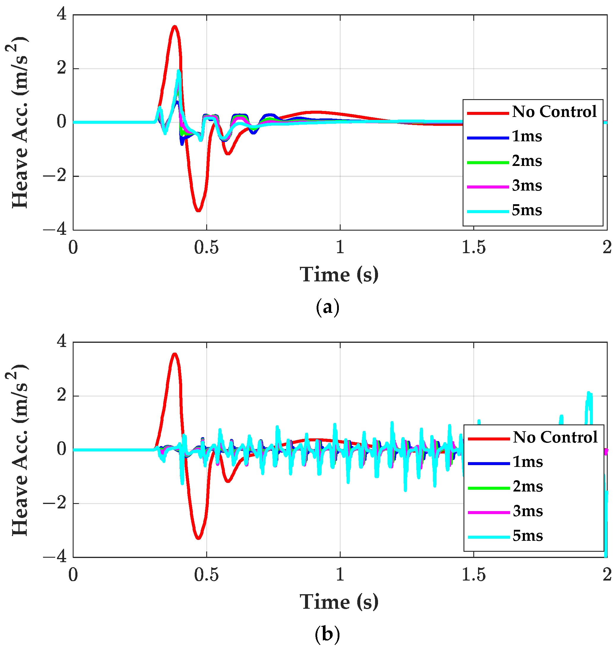
3.3. Simulation on Half-Sine Bump and Sine-Waved Road

In this subsection, the controllers are simulated on the half-sine bump and sine-waved road. The six controllers, LQR, LQSOF, FSFSBOM, SOFSBOM, PACRLS, and PACEKF, are simulated and compared in terms of ride comfort and control effort.
The first simulation is performed with LQR, LQSOF, FSFSBOM, and SOFSBOM. Figure 6, Figure 7, Figure 8 and Figure 9 show the simulation results of the no control case and four controllers on the half-sine bump and sine-waved road. In those figures, FSFSBOM.HSB and SOFSBOM.HSB stand for FSFSBOM and SOFSBOM designed on the half-sine bump, respectively. In those figures, FSFSBOM.SWR and SOFSBOM.SWR stand for FSFSBOM and SOFSBOM designed on the sine-waved road, respectively.
As shown in those figures, LQR, LQSOF, SOFSBOM.HSB, and SOFSBOM.SWR provided nearly similar results to one another. This means that SOF controllers designed with the structure of (11) will show nearly identical performance in terms of ride comfort. On the other hand, FSFSBOMs, i.e., FSFSBOM.HSB and FSFSBOM.SWR, outperform the other SOF controllers. However, FSFSBOM.SWR shows chattering in its response, as shown in Figure 7. This is caused by the high gain on the vertical velocity of the SPM, as given in Table 3.
The second simulation is performed with SOFSBOM, PACRLS, and PACEKF. In PACRLS, the forgetting factors were set to 0.999 and 0.8 for the half-sine bump and sine-waved road, respectively. In PACEKF, the covariance matrices, M and N, were set as 104·I4×4 and 1, respectively. This set was determined by trial and error. This set means that EKF prefers sensor measurement instead of the system dynamics. If the multiplier, i.e., 104, is less than 102, then the performance of EKF will be deteriorated.
Figure 10 and Figure 11 show the simulation results of the no control case and SOFSBOM, PACRLS, and PACEKF on the half-sine bump and sine-waved road. As shown in those figures, LQSOF and SOFSBOM show nearly similar performance, as expected from Figure 5.
As shown in Figure 10, SOFSBOM.HSB and PACRLS on the half-sine bump show nearly identical results to each other. On the other hand, PACEKF shows the best result in terms of ride comfort. This is caused by the fact that M was set to a higher value. If M is set to a lower value of 10 or 1, PACEKF will give a similar result to PACRLS. Instead of reducing M, if the forgetting factor, λ, of PACRLS is set a value less than 0.99, PACRLS will show identical behavior to PACEKF. As shown in Figure 10, PACEKF did not converge to zero due to no damping and very fast learning rate.
The plots of the spring stiffness and damping coefficient as given in Figure 10c,d show that those parameters converged into the gains of SOFSBOM.HSB. This is caused by the fact that the spring and damping force curves given in Figure 4 are nearly linear. For the same reason, if there are severe nonlinearities in spring and damper, the control performance of PACRLS and PACEKF will be deteriorated.
As shown in Figure 11, PACRLS and PACEKF outperform the SOF controllers, LQSOF and SOFSBOM.SWR. This is caused by the fact that the sine-wave road is a periodic disturbance, and that the forgetting factor of RLS was set to 0.8, which means RLS has short memory on history.
The simulation results given in Figure 10 and Figure 11 mean that SOFSBOM and PAC try to make the suspension force be zero, as given in (14), with the identical control structure. This also means that only two signals, i.e., the suspension stroke and its rate, are needed for SOFSBOM and PAC and that only two gains are needed for ride comfort. In addition to the identical control structure, the performances of SOFSBOM and PAC are equivalent to each other in terms of ride comfort on the half-sine bump, as shown in Figure 10, and PAC outperforms LQSOF and SOFSBOM on the sine-waved road, as shown in Figure 11.
The third simulation is performed with PACEKF for several sampling periods. Generally, the smaller the sampling periods, the better the control performance. However, the sampling period is limited for a suspension controller due to the small computational capacity of a microprocessor. In the third simulation, PACRLS and PACEKF are simulated with the sampling periods of 1, 2, 5, 10 ms.
Figure 12 shows the simulation results of PACRLS and PACEKF with various sampling periods. As shown in Figure 12, the control performance is deteriorated as the sampling period becomes larger for PACRLS. This is natural that the PACRLS cannot reject the high-frequency components in the disturbance. In the case of PACEKF, the control performance was not deteriorated as the sampling period became larger. However, it did not converge to zero. As shown in Figure 12b, the response of PACEKF will diverge if the sampling period is equal to or larger than 5 ms. For this reason, if one wants to achieve desirable performance, then the sampling period of PAC should be smaller than 5 ms.
The fourth simulation is performed with PACEKF for several actuator bandwidths. Generally, the larger the bandwidth, the better the control performance. However, actuators used for vehicle suspension have very small bandwidth due to physical limitations. In the third simulation, PACRLS and PACEKF are simulated with the bandwidths of 5, 10, 50, 100 Hz. The sampling periods of PACs were set to 1 ms.
Figure 13 shows the simulation results of PACRLS and PACEKF with various actuator bandwidths. As shown in Figure 13, the control performance is severely deteriorated as the bandwidth of the actuator becomes smaller. If one wants to achieve desirable performance, then the bandwidth of the actuator should be larger than 50 Hz. Different from the results given in Figure 10, the heave accelerations of PACEKF with the bandwidths of 5 and 10 Hz converged into zero due to low bandwidth.
The fifth simulation is performed with different dampers. Figure 14 shows several damper characteristics: Damper#1, Damper#2, Damper#3, and Damper#4. As shown in Figure 14, Damper#1 is a soft damper, and Damper#4 is a hard one. It is natural that the harder the damper, the lower the performance in terms of ride comfort. Moreover, high slope near zero velocity acts as friction as shown in Damper#4, Figure 14. The other parameters are identical to those given in Table 1 and Figure 4a. The sampling periods of PACs were set to 1 ms, and the actuator bandwidth was set to 10 Hz.
Figure 15 and Figure 16 show the simulation results of PACRLS and PACEKF. As shown in these figures, the harder the damper, the lower the performance in terms of ride comfort. This is natural that the soft damper can give better ride comfort than the hard one.

4. Conclusions

This paper presents the design methods of active suspension controllers, PAC and SOF ones, with the quarter-car model and two available sensor signals. The control objective is to make the suspension force between the SPM and USPM be zero to improve ride comfort. For this purpose, the suspension stroke and its rate were selected as a sensor output for SOF controllers. The quarter-car model was selected as a vehicle model. To avoid the full-state measurement of LQR, SOF control was adopted as a controller structure. The SOF controllers were designed with LQ cost function and the SBOM. With the sensor signals, PAC was designed with RLS and EKF for the purpose of making the suspension force be zero. To compare the performance of those controllers in terms of ride comfort, simulation was performed on the half-sine bump and sine-waved road in the MATLAB/Simulink environment. From simulation results, the following points were identified.
  • The SOF controllers designed with SBOM and PAC have identical control structure and show equivalent performance to each other in terms of ride comfort.
  • FSFSBOM designed on the half-sine bump outperforms the other SOF controllers.
  • PACRLS and PACEKF show equivalent performance to the SOF controllers on the half-sine bump in terms of ride comfort. On the other hand, PAC outperforms the other SOF controllers under periodic disturbances such as the sine-waved road.
  • The sampling period and the actuator bandwidth of PACs play a critical role in controlling the active suspension. For desired performance, the sampling period of PAC should be less than 5 ms and actuator bandwidth should be larger than 50 Hz.
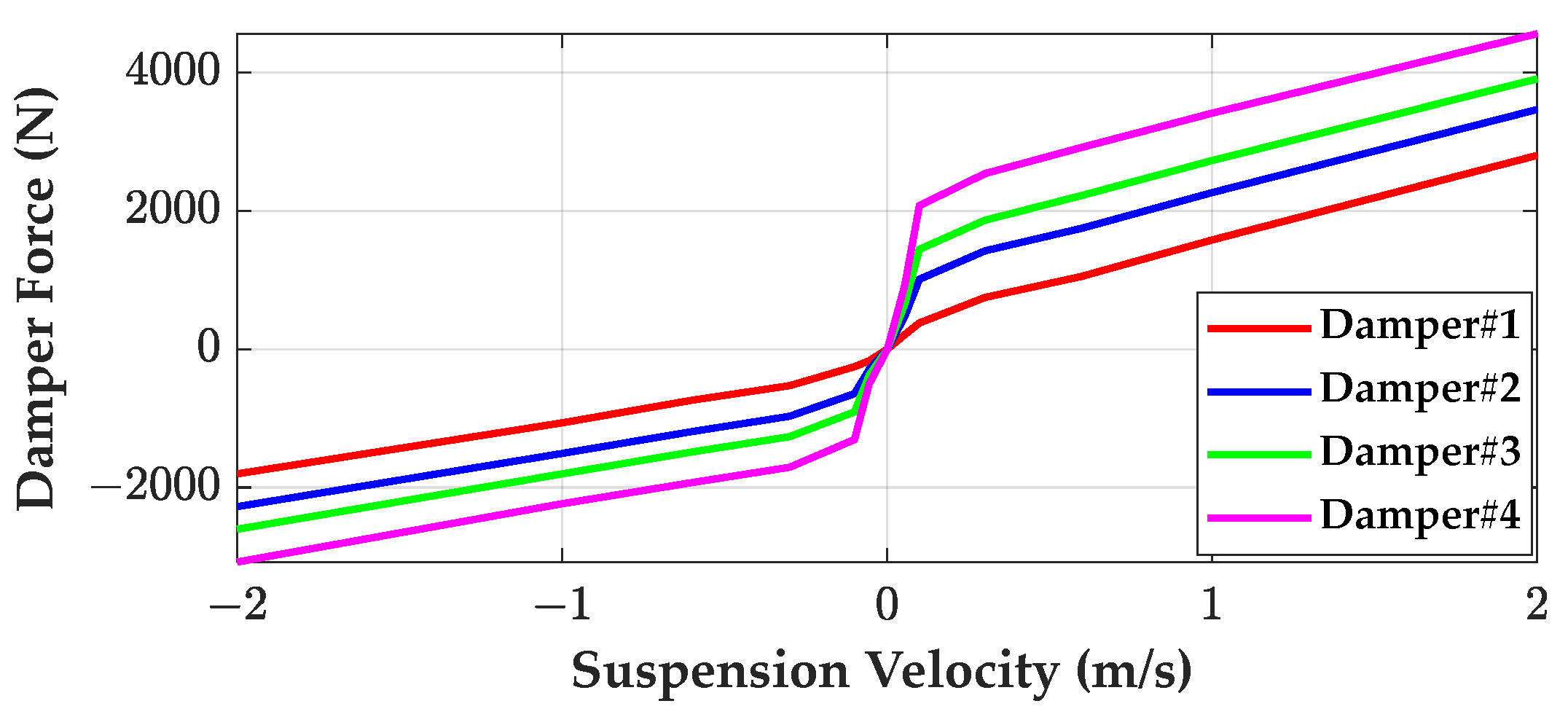
  • If the damper has high damping coefficients, the control performance of PAC, i.e., PACRLS and PACEKF, is deteriorated.
To achieve that the suspension force becomes zero with a controller, several methods can be applied. For example, learning-based controllers such as fuzzy learning and neural networks can be applied to tune the spring stiffness and the damping coefficient. In addition, to validate the proposed SOFCs and PAC in this paper, experiments with the controllers designed in this paper can be conducted on a small-scaled quarter-car test rig/bench.
The drawback of the proposed method is that it was designed only for ride comfort improvement by canceling the suspension force transmitted into the SPM. In future work, an SOF controller and PAC will be designed for compromising on conflicting ride comfort and road holding by modifying the structure of SOF controllers and PAC to include the tire deflection.

Funding

This work was supported by the Ministry of Education through the National Research Foundation of Korea (NRF) under the Basic Science Research Program (RS-2019-NR040071).

Data Availability Statement

The original contributions presented in this study are included in the article. Further inquiries can be directed to the corresponding author.

Conflicts of Interest

The authors declare no conflicts of interest.

Abbreviations

The following abbreviations are used in this manuscript:
EKFExtended Kalman filter
FSFFull-state feedback
HSBHalf-sine bump
LQRLinear quadratic regulator
LQ SOFLinear quadratic static output feedback
SBOMSimulation-based optimization method
SOFStatic output feedback
SOFCStatic output feedback controller
SPMSprung mass
PACParameter adaptive controller
PACEKFParameter adaptive controller with recursive least square
PACRLSParameter adaptive controller with extended Kalman filter
RLSRecursive least square
SWRSine-waved road
USPMUnsprung mass
Nomenclature
bsdamping coefficient of a damper within a suspension (N·s/m)
fsuspension force acting on sprung and unsprung masses
JLQ cost function used for LQR, LQSOF, and LQSSOF
JScost function of the simulation-based optimization
ksstiffness of a spring within a suspension (N/m)
ktstiffness of a tire (N/m)
mssprung mass (kg)
muunsprung mass under a suspension (kg)
uforces generated by an actuator within a suspension (N)
zrroad elevation acting on a tire (m)
zsvertical displacement of a sprung mass (m)
zuvertical displacement of a wheel center (m)
ξimaximum allowable value (MAV) of a weight in LQ cost function
λforgetting factor in the recursive least square
ριweight in LQ cost function

References

  1. Sharp, R.S.; Crolla, D.A. Road vehicle suspension system design—A review. Veh. Syst. Dyn. 1987, 16, 167–192. [Google Scholar] [CrossRef]
  2. Hrovat, D. Survey of advanced suspension developments and related optimal control applications. Automatica 1997, 33, 1781–1817. [Google Scholar] [CrossRef]
  3. Tseng, H.E.; Hrovat, D. State of the art survey: Active and semi-active suspension control. Veh. Syst. Dyn. 2015, 53, 1034–1062. [Google Scholar] [CrossRef]
  4. ISO 2631-1:1997; Mechanical Vibration and Shock—Evaluation of Human Exposure to Whole-Body Vibration—Part 1: General Requirements. International Organization for Standardization: Geneva, Switzerland, 1997.
  5. Wilson, D.A.; Sharp, R.S.; Hassan, S.A. The application of linear optimal control theory to the design of active automobile suspensions. Veh. Syst. Dyn. 1987, 15, 105–118. [Google Scholar] [CrossRef]
  6. Cao, D.; Song, X.; Ahmadian, M. Editors’ perspectives: Road vehicle suspension design, dynamics, and control. Veh. Syst. Dyn. 2011, 49, 3–28. [Google Scholar] [CrossRef]
  7. Theunissen, J.; Tota, A.; Gruber, P.; Dhaens, M.; Sorniotti, A. Preview-based techniques for vehicle suspension control: A state-of-the-art review. Annu. Rev. Control 2021, 51, 206–235. [Google Scholar] [CrossRef]
  8. Sun, W.; Pan, H.; Zhang, Y.; Gao, H. Multi-objective control for uncertain nonlinear active suspension systems. Mechatronics 2014, 24, 318–327. [Google Scholar] [CrossRef]
  9. Hac, A. Optimal linear preview control of active vehicle suspension. Veh. Syst. Dyn. 1992, 21, 167–195. [Google Scholar] [CrossRef]
  10. Guo, L.; Zhang, L. Robust H control of active vehicle suspension under non-stationary running. J. Sound Vib. 2012, 331, 5824–5837. [Google Scholar] [CrossRef]
  11. Sun, W.; Gao, H.; Kaynak, O. Adaptive backstepping control for active suspension systems with hard constraints. IEEE/ASME Trans. Mechatron. 2013, 18, 1072–1079. [Google Scholar] [CrossRef]
  12. Chen, S.-A.; Wang, J.-C.; Yao, M.; Kim, Y.-B. Improved optimal sliding mode control for a non-linear vehicle active suspension system. J. Sound Vib. 2017, 395, 1–25. [Google Scholar] [CrossRef]
  13. Pan, H.; Sun, W.; Jing, X.; Gao, H.; Yao, J. Adaptive tracking control for active suspension systems with non-ideal actuators. J. Sound Vib. 2017, 399, 2–20. [Google Scholar] [CrossRef]
  14. Yatak, M.O.; Sahin, F. Ride comfort-road holding trade-off improvement of full vehicle active suspension system by interval type-2 fuzzy control. Eng. Sci. Technol. Int. J. 2021, 24, 259–270. [Google Scholar] [CrossRef]
  15. Park, M.; Yim, S. Design of static output feedback and structured controllers for active suspension with quarter-car model. Energies 2021, 14, 8231. [Google Scholar] [CrossRef]
  16. Jeong, Y.; Sohn, Y.; Chang, S.; Yim, S. Design of static output feedback controllers for an active suspension system. IEEE Access 2022, 10, 26948–26964. [Google Scholar] [CrossRef]
  17. Kim, J.; Yim, S. Design of a suspension controller with an adaptive feedforward algorithm for ride comfort enhancement and motion sickness mitigation. Actuators 2024, 13, 315. [Google Scholar] [CrossRef]
  18. Attia, T.; Vamvoudakis, K.G.; Kochersberger, K.; Bird, J.; Furukawa, T. Simultaneous dynamic system estimation and optimal control of vehicle active suspension. Veh. Syst. Dyn. 2019, 57, 1467–1493. [Google Scholar] [CrossRef]
  19. Jeong, Y.; Sohn, Y.; Chang, S.; Yim, S. Design of virtual reference feedforward controller for an active suspension system. IEEE Access 2022, 10, 65671–65684. [Google Scholar] [CrossRef]
  20. Kim, J.; Yim, S. Design of static output feedback suspension controllers for ride comfort improvement and motion sickness reduction. Processes 2024, 12, 968. [Google Scholar] [CrossRef]
  21. Bryson, A.E., Jr.; Ho, Y. Applied Optimal Control; Hemisphere: New York, NY, USA, 1975. [Google Scholar]
  22. Hansen, N.; Muller, S.D.; Koumoutsakos, P. Reducing the time complexity of the derandomized evolution strategy with covariance matrix adaptation (CMA-ES). Evol. Comput. 2003, 11, 1–18. [Google Scholar] [CrossRef]
  23. Wenzel, T.A.; Burnham, K.J.; Blundell, M.V.; Williams, R.A. Dual extended Kalman filter for vehicle state and parameter estimation. Veh. Syst. Dyn. 2006, 44, 153–171. [Google Scholar] [CrossRef]
  24. Jiang, K.; Victorino, A.C.; Charara, A. Adaptive estimation of vehicle dynamics through RLS and Kalman filter approaches. In Proceedings of the 2015 IEEE 18th International Conference on Intelligent Transportation Systems, Canary Islands, Spain, 15–18 September 2015; pp. 1741–1746. [Google Scholar] [CrossRef]
  25. Hu, D.; Zong, C.; Na, X. Combined estimation of vehicle states and road friction coefficients using dual extended Kalman filter. Chin. J. Mech. Eng. 2013, 26, 313–324. [Google Scholar] [CrossRef]
  26. Park, M.; Yim, S. Design of robust observers for active roll control. IEEE Access 2019, 7, 173034–173043. [Google Scholar] [CrossRef]
  27. Haykin, S. Adaptive Filter Theory, 2nd ed.; Prentice-Hall: Hoboken, NJ, USA, 1991; pp. 760–761. [Google Scholar]
  28. Mechanical Simulation Corporation. CarSim Data Manual, Version 8; Mechanical Simulation Corporation: Ann Arbor, MI, USA, 2009.
Figure 1. Schematic diagram of SOFC and PAC.
Actuators 14 00150 g001
Figure 2. Quarter-car model.
Actuators 14 00150 g002
Figure 3. Simulation-based optimization procedure.
Actuators 14 00150 g003
Figure 4. Spring and damping curves of the quarter-car model. (a) Spring force; (b) damping force.
Actuators 14 00150 g004
Figure 5. Frequency responses of the SOF controllers from the road profile to the heave acceleration of SPM. (a) SOF controllers designed on HSB; (b) SOF controllers designed on SWR.
Actuators 14 00150 g005
Figure 6. Simulation results of no control case and four controllers which were designed on the HSB on the HSB. (a) Heave acceleration of the SPM; (b) control inputs.
Actuators 14 00150 g006
Figure 7. Simulation results of no control case and four controllers which were designed on SWR on the HSB. (a) Heave acceleration of the SPM; (b) control inputs.
Actuators 14 00150 g007
Figure 8. Simulation results of no control case and four controllers which were designed on HSB on the SWR. (a) Heave acceleration of the SPM; (b) control inputs.
Actuators 14 00150 g008
Figure 9. Simulation results of no control case and four controllers which were designed on SWR on the SWR. (a) Heave acceleration of the SPM; (b) control inputs.
Actuators 14 00150 g009
Figure 10. Simulation results of no control case and SOFSBOM, PACRLS, and PACEKF on the HSB. (a) Heave acceleration of the SPM; (b) control inputs; (c) variation of spring stiffness; (d) variation of damping coefficient.
Actuators 14 00150 g010aActuators 14 00150 g010b
Figure 11. Simulation results of no control case and SOFSBOM, PACRLS, and PACEKF on the SWR. (a) Heave acceleration of the SPM; (b) control inputs; (c) variation of spring stiffness; (d) variation of damping coefficient.
Actuators 14 00150 g011aActuators 14 00150 g011b
Figure 12. Simulation results of no control case, PACRLS, and PACEKF for various sampling periods on the HSB. (a) Heave acceleration of the SPM with PACRLS; (b) heave acceleration of the SPM with PACEKF.
Actuators 14 00150 g012
Figure 13. Simulation results of no control case, PACRLS, and PACEKF for various bandwidths on the HSB. (a) Heave acceleration of the SPM with PACRLS; (b) heave acceleration of the SPM with PACEKF.
Actuators 14 00150 g013
Figure 14. Damping force curves of Damper#1, Damper#2, Damper#3, and Damper#4.
Actuators 14 00150 g014
Figure 15. Simulation results of PACRLS with various dampers. (a) Heave acceleration of the SPM; (b) control input.
Actuators 14 00150 g015
Figure 16. Simulation results of PACEKF with various dampers. (a) Heave acceleration of the SPM; (b) control input.
Actuators 14 00150 g016
Table 1. Parameters of the quarter-car model [15].
ParameterValueParameterValue
ms413 kgmu45 kg
ks34,000 N/mbs3500 N·s/m
kt230,000 N/m
Table 2. MAVs in LQ cost function.
MAVValueMAVValue
ξ11 m/s2ξ20.1 m
ξ30.01 mξ43000 N
Table 3. Gain matrices of the controllers.
ControllerRoad ProfileGain Matrix
LQR K = 14 , 073 9481 373 1097
LQSOF G = 16 , 061 1080
FSFSBOMHSB K = 8955 16 , 845 4934 1307
SOFSBOMHSB G = 15 , 585 1377
FSFSBOMSWR K = 20 , 000 15 , 003 100 , 000 1444
SOFSBOMSWR G = 19 , 380 656
Disclaimer/Publisher’s Note: The statements, opinions and data contained in all publications are solely those of the individual author(s) and contributor(s) and not of MDPI and/or the editor(s). MDPI and/or the editor(s) disclaim responsibility for any injury to people or property resulting from any ideas, methods, instructions or products referred to in the content.

