Article

Prescribed Performance Tracking Control for Nonlinear Stochastic Time-Delay Systems with Multiple Constraints

School of Automation and Software Engineering, Shanxi University, Taiyuan 030006, China
*
Author to whom correspondence should be addressed.
Actuators 2025, 14(1), 19; https://doi.org/10.3390/act14010019
Submission received: 25 November 2024 / Revised: 27 December 2024 / Accepted: 6 January 2025 / Published: 8 January 2025
(This article belongs to the Section Control Systems)

Abstract

:
This paper proposes a prescribed performance tracking control scheme for a category of nonlinear stochastic time-delay systems with input saturation and state asymmetric time-varying constraints. First, to solve the non-differentiable problem caused by input saturation, a smooth nonlinear function was utilized to approximate the saturation function. A nonlinear mapping technique was employed to transform the constrained problem into a bounded convergence problem. The time-delay problem was then solved by constructing the corresponding Lyapunov–Krasovskii function. The error feedback controller was constructed by combining the backstepping technique, the dynamic surface technique, the neural network approximation technique, and the adaptive control method. Based on stochastic mean-square stability theory, all signals in the closed-loop system are proven to be bounded under the designed control scheme. Also, this scheme ensures that the system states always stay within the constraint range, and the tracking error meets the prescribed performance constraint. Finally, the feasibility and superiority of the proposed control scheme were validated through simulation.

1. Introduction

Stochastic time-delay systems, which consider both random disturbances and time-delay factors, are playing an increasingly crucial role in various fields, such as physics, biology, engineering, medicine, social sciences, economics, finance, etc. [1,2,3]. Since random disturbances and system time delays can seriously affect system stability, the stability and stabilization problems of such systems have attracted widespread concern from scientists and experts across all fields of natural sciences, yielding rich research results. References [4,5] investigated the stability problem of stochastic nonlinear systems with unknown time delay and disturbances, and the global asymptotic stability criterion and local exponential stability criterion were given separately, providing a valuable theoretical basis for the controller design of stochastic time-delay systems. Based on these important stability research results, References [6,7] presented the finite-time stabilization control scheme for stochastic time-delay systems. Nevertheless, restrictions, which widely exist in practical systems (e.g., state constraints, output constraints, and input constraints), lead to increased difficulty in the controller design, which affects the development of control theory for stochastic time-delay systems.
In fact, many systems, such as the wheeled mobile robot (WMR) systems [8,9,10], where the maximum forward speeds of the wheels are limited to a certain range, and the chemical reactor systems [11,12], where the reactant concentrations and feed rates are also constrained within a specific range, are restricted by constraints. As a result, dealing with constraints in controller design is an important task. For this problem, Reference [13] proposed a barrier Lyapunov function (BLF) that can produce values close to infinity as its parameters verge on certain limits. By using the BLF approach, References [14,15] pioneered a control scheme for nonlinear systems with only output constraints. Nevertheless, the virtual controllers designed by using this method should satisfy the “feasibility condition”, i.e., if the particular constraints can be met, the virtual controllers will be workable. It makes the design and application of the relevant control solutions highly difficult. Subsequently, the barrier-function-based nonlinear mapping technique was developed in place of the BLF approach, avoiding the judgment of feasibility [16,17]. However, compared to deterministic systems, few results have been obtained in the study of constrained control problems for nonlinear stochastic time-delay systems. In Reference [18], the stabilization problem of nonlinear stochastic systems suffering asymmetric output constraints was examined by combining the BLF method and backstepping technique. Despite this, the focus of the study was solely on the output constraints. For the full-state-constrained case, Reference [19] solved the adaptive tracking problem of nonlinear stochastic time-delay systems with the construction of symmetric and asymmetric BLFs.
Meanwhile, it is worth noting that input saturation degrades control performance and even destabilizes the system, however, this is inevitable in practical systems. Recently, the design of the controller subjected to input saturation has been addressed in the following ways: either by utilizing a smooth function to approach the input saturation, as seen in References [20,21,22], or by introducing an auxiliary system, as demonstrated in Reference [23]. To the authors’ knowledge, research related to the tracking control of nonlinear stochastic time-delay systems with input saturation and time-varying full-state constraints still needs to be investigated more comprehensively. Therefore, enhancing the control performance of the aforementioned systems constitutes a focal point of this paper.
To hasten the convergence speed and accuracy of the system, scholars have proposed some effective methods, such as finite-time control [24,25], time synchronization control [26], and prescribed performance control [27,28,29]. Among them, the prescribed performance control strategy can guarantee that the tracking error meets the prescribed performance requirements, so it has captured a great deal of attention. Lately, experts have optimized the prescribed performance control methods from different aspects. For example, References [30,31,32] put forward a finite-time performance function, which allowed the tracking error to converge to a more diminutive fixed region within the confines of finite time. Reference [33] investigated a prescribed performance control problem of nonlinear strict-feedback systems subject to actuator faults. Reference [34] introduced a new constraint handling technique that overcomes the limitation requiring the absolute value of the initial value of the performance boundary function to be larger than the absolute value of the initial value of the tracking error. Nevertheless, the development of prescribed performance tracking control for stochastic time-delay systems is progressing more slowly than for deterministic systems. Improving and developing advanced tracking control for nonlinear stochastic time-delay systems remains challenging.
Given the above discussion, this paper provides a prescribed performance tracking control design scheme for a category of nonlinear stochastic time-delay systems with state asymmetric time-varying constraints and input saturation constraints. The main contributions are as follows:
(1) Unlike the stochastic time-delay systems researched in [35,36,37], the controlled system is more general and applicable to a wider range of practical scenarios [38,39,40].
(2) Compared to the state-constrained control methods proposed in [30,31,32], this paper proposes a new barrier function-based nonlinear mapping technique. It overcomes the limitation of the signs of the constraint boundary functions being fixed. So it is more effective than [30,31,32] in handling general constraints.
(3) Unlike [41,42,43,44], the designed controller not only ensures that the system states consistently meet the asymmetric time-varying constraints, but also guarantees that the system output can track the reference signal within a preset time, achieving good transient and steady-state tracking performance. So, the performance requirements of real-world physical systems are satisfiable by the proposed controller.

2. Problem Description and Preliminaries

2.1. Problem Description

The following nonlinear stochastic time-delay system is considered as follows:
d x i = g i ( x ¯ i ) x i + 1 + f i ( x ¯ i ) + ψ i x ¯ i ( t τ i ) d t + φ i T ( x ¯ i ) d ω , i = 1 , 2 , , n 1 d x n = g n ( x ¯ n ) u ( v ) + f n ( x ¯ n ) + ψ n x ¯ n ( t τ n ) d t + φ n T ( x ¯ n ) d ω , y = x 1 ,
where x ¯ i = [ x 1 , x 2 , , x i ] T R i denotes the system state vector, and y signifies the system output. x ¯ i ( t τ i ) = [ x 1 ( t τ 1 ) , , x i ( t τ i ) ] T R i denotes the state-delay vector, and τ i signifies the time-delay term. g i ( · ) , f i ( · ) , and φ i ( · ) denote unknown and smooth nonlinear functions, while ψ i ( · ) with ψ i ( 0 ) = 0 denotes an unknown and smooth-bounded nonlinear time-delay function. ω signifies an r-dimension standard Wiener process. u ( v ) denotes the actual control input subjected to the saturation constraint, which is expressed as follows:
u ( v ) = u P , v u P v , u S < v < u P u S , v u S
where u P > 0 and u S < 0 represent the known constants, and v indicates the desired control law that needs to be designed.
We take the following asymmetric time-varying state constraints into account:
x i R i c i l ( t ) < x i < c i h ( t ) , i = 2 , , n ,
where the initial value of state x i satisfies x i ( 0 ) R i , c i l ( t ) denotes the lower constraint function, and c i h ( t ) denotes the upper constraint function. Thus, there exists a constant d i , such that we have the following:
c i h ( t ) c i l ( t ) d i > 0 , i = 2 , , n .
For system (1), the objective is to design a tracking controller, such that we have the following: (1) all signals of the closed-loop system are bounded. (2) The system states always satisfy the pre-described constraints, even if the signs of the constraint boundary functions change. (3) The system output y ( t ) is capable of tracking the reference signal y d ( t ) before a specified timeframe, and the tracking error e ( t ) , defined as y ( t ) y d ( t ) , conforms to the prescribed performance constraint.
The following assumptions and definitions are needed for the sake of achieving the above control objectives.

2.2. Preliminaries

Assumption 1. 
g i ( · ) is a smooth and bounded unknown nonlinear function, assuming its sign is known, and there exist positive constants g 0 and g M , such that g i ( · ) satisfies 0 < g 0 g i ( · ) g M .
Assumption 2. 
The reference signal y d and the derivatives of all orders are continuously bounded.
Definition 1 
([45]). For the stochastic system d x = f ( x ) d t + I ( x ) d ω , the stochastic differential operator L of the differentiable function V ( x ) is denoted by the following formula:
L V ( x ) = V ( x ) x f ( x ) + 1 2 T r I T 2 V ( x ) x 2 I
where the function V ( x ) is positive-definite and satisfies the specified condition V ( x ) C 2 , and T r ( A ) denotes the trace of A.
Lemma 1 
([46,47]). As for the smooth bounded nonlinear time-delay function ψ i ( · ) , there exist positive smooth functions m i l ( x l ( · ) ) , satisfying m i l ( 0 ) = 0 , such that the following equation holds:
| ψ i ( · ) | l = 1 i m i l ( x l ( · ) ) , i = 1 , , n .
Lemma 2 
([41]). Let F ( Z ) be a smooth continuous function defined on Ω; there is a radial basis function (RBF) NN described as F n n ( Z ) = W * T Ξ ( Z ) , satisfying the following:
F ( Z ) = W * T Ξ ( Z ) + δ ( Z ) , sup Z Ω | F ( Z ) W * T Ξ ( Z ) | Δ ,
where W * T denotes the optimal weight vector, Ξ ( Z ) denotes the basis function, δ ( Z ) denotes the approximation error with | δ ( Z ) | Δ , and Δ denotes a positive constant.
Lemma 3 
([48]). Suppose A and B are non-negative real numbers and there are positive constants K and D that satisfy 1 K + 1 D = 1 , then the following inequality holds:
A B A K K + B D D ,
Lemma 4 
([49]). For the stochastic system described by d x = f ( x ) d t + I ( x ) d ω , considering x R n and t > t 0 , suppose there exists a positive-definite function V ( x , t ) : R n × R + R + ; two constants, C > 0 and D > 0 ; and class K -functions K 1 and K 2 , such that we have the following:
K 1 ( x ) V ( x , t ) K 2 ( x ) ,
L V ( x , t ) C V + D .
Then, there exists a unique solution to the stochastic system and it has the following:
E ( V ( x , t ) ) V ( x ( 0 ) ) e x p ( C t ) + D C , t > t 0 .
where E ( · ) indicates the mathematical expectation.

3. Solutions to Constraints

In this section, we present solutions for saturated input, prescribed performance constraints, and asymmetric time-varying state constraints, respectively. To simplify the description, the independent variables t and x ¯ i will be omitted.

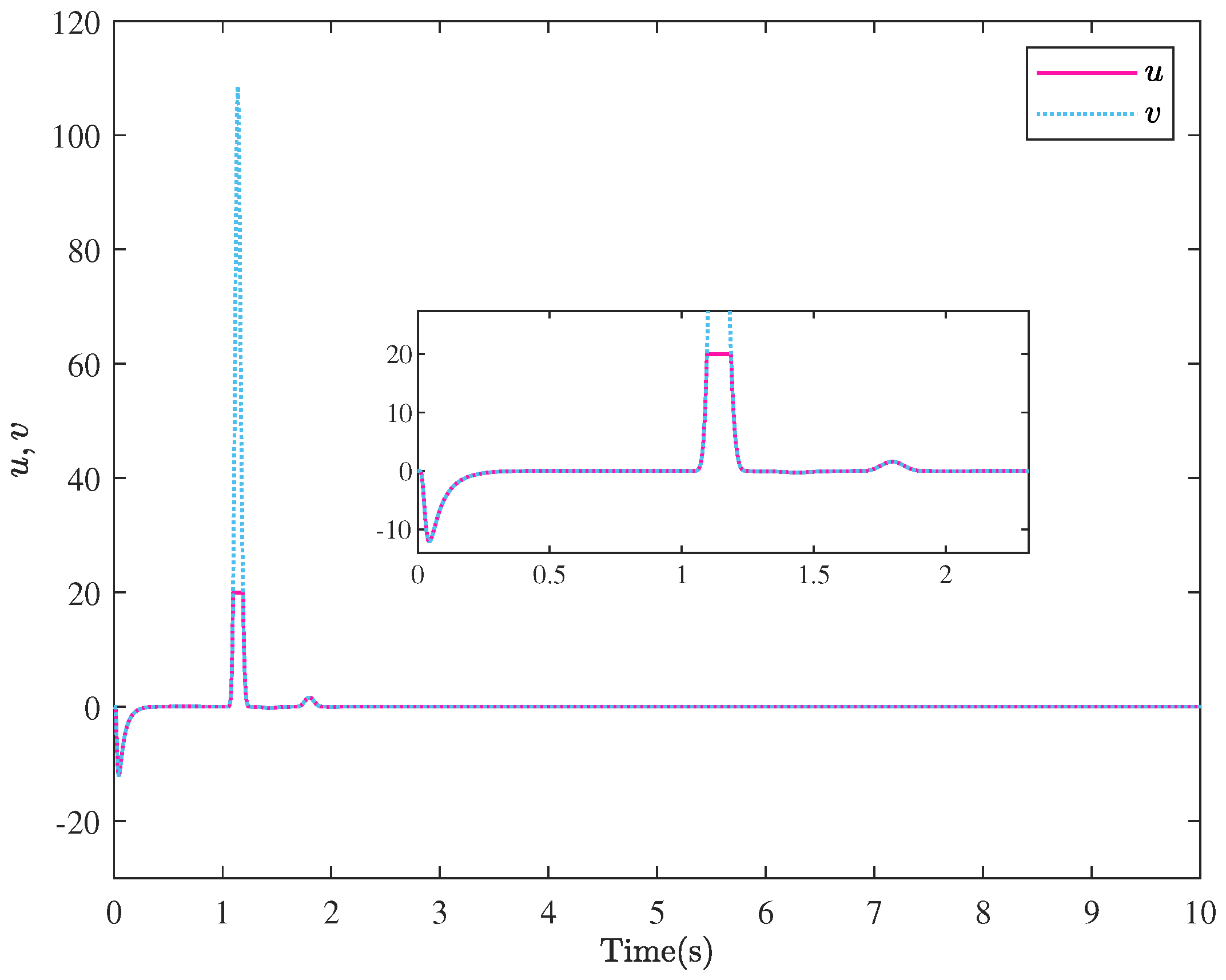
3.1. Input Saturation Constraint

From Equation (2), it can be seen that there exist non-differentiable points in u ( v ) , which makes it impossible to design the controller directly by the backstepping technique. To solve this problem, the saturation function u ( v ) is approximated using a smooth segmented function k ( v ) in this paper. k ( v ) is shown as follows:
k ( v ) = u P tanh ( v u P ) , v 0 u S tanh ( v u S ) , v < 0
where the approximation error is defined as q ( v ) = u ( v ) k ( v ) , and | q ( v ) | m a x { u P ( 1 tanh ( 1 ) ) , u S ( tanh ( 1 ) 1 ) } = Q . Based on the differential median theorem, take any point v in ( v 0 , v ) on k ( v ) (i.e., v = h v + ( 1 h ) v 0 , 0 < h < 1 ) , so that the equation k ( v ) = k ( v 0 ) + k v · ( v v 0 ) holds, where k v = k ( v ) v | v = v . When v 0 = 0 , one has k ( v ) = k v v .
Remark 1. 
When v 0 , k v 4 ( e x p ( v u P ) + e x p ( v u P ) ) 2 and k v 4 ( e x p ( v u S ) + e x p ( v u S ) ) 2 when v < 0 . It is clear from the analysis that the maximum value of k v can be obtained at v = 0 , so there is a constant k m , which is unknown and positive, satisfying 0 < k m < k v 1 . It is worth noting that k m cannot be used for the controller design. It is only suitable for stability analysis.

3.2. Prescribed Performance Constraint

The third control objective of this paper can be stated as follows:
ϱ ( t ) < e < ϱ ( t ) , t 0
where e = y y d denotes the tracking error, is a normal number, and ϱ ( t ) denotes the performance function. To ensure that the systems have good transient and steady-state tracking performance, in this paper, the performance function is designed in advance as follows:
ϱ ( t ) = ϱ 0 t T f exp 1 T f T f t + ϱ T f t [ 0 , T f ) , ϱ T f t [ T f , + ) ,
where ϱ 0 , T f , and ϱ T f are positive constants that need to be designed in advance.
Remark 2. 
Encouraged by [50], ϱ ( t ) , the finite-time performance function (FTPF) is a smooth function and exhibits the following three elements: (i) ϱ ˙ ( t ) 0 ; (ii) ϱ ( t ) > 0; (iii) lim t T f ϱ ( t ) = ϱ T f > 0 , and ϱ ( t ) = ϱ T f , for any t T f with T f being the settling time. Different from the traditional and monotonically decreasing performance function ϱ ( t ) = ( ϱ 0 ϱ ) e x p ( l 1 t ) + ϱ , which can only assure that the tracking error is often required to achieve convergence when t + , the new method can ensure that the system converges in T f .
To ensure that the tracking error fulfills the preset performance requirement, i.e., to satisfy Equation (13), it is necessary to construct the following nonlinear mapping function, as follows:
μ 1 = e ( c 1 h e ) ( e c 1 l ) ,
where c 1 h = ϱ , c 1 l = ϱ , and c 1 l ( 0 ) < e ( 0 ) < c 1 h ( 0 ) . From Equation (15), it follows that if c 1 l ( 0 ) < e ( 0 ) < c 1 h ( 0 ) , then μ 1 + as e c 1 h , and μ 1 as e c 1 l . Thus, by making μ 1 bounded, it is guaranteed that c 1 l < e < c 1 h .

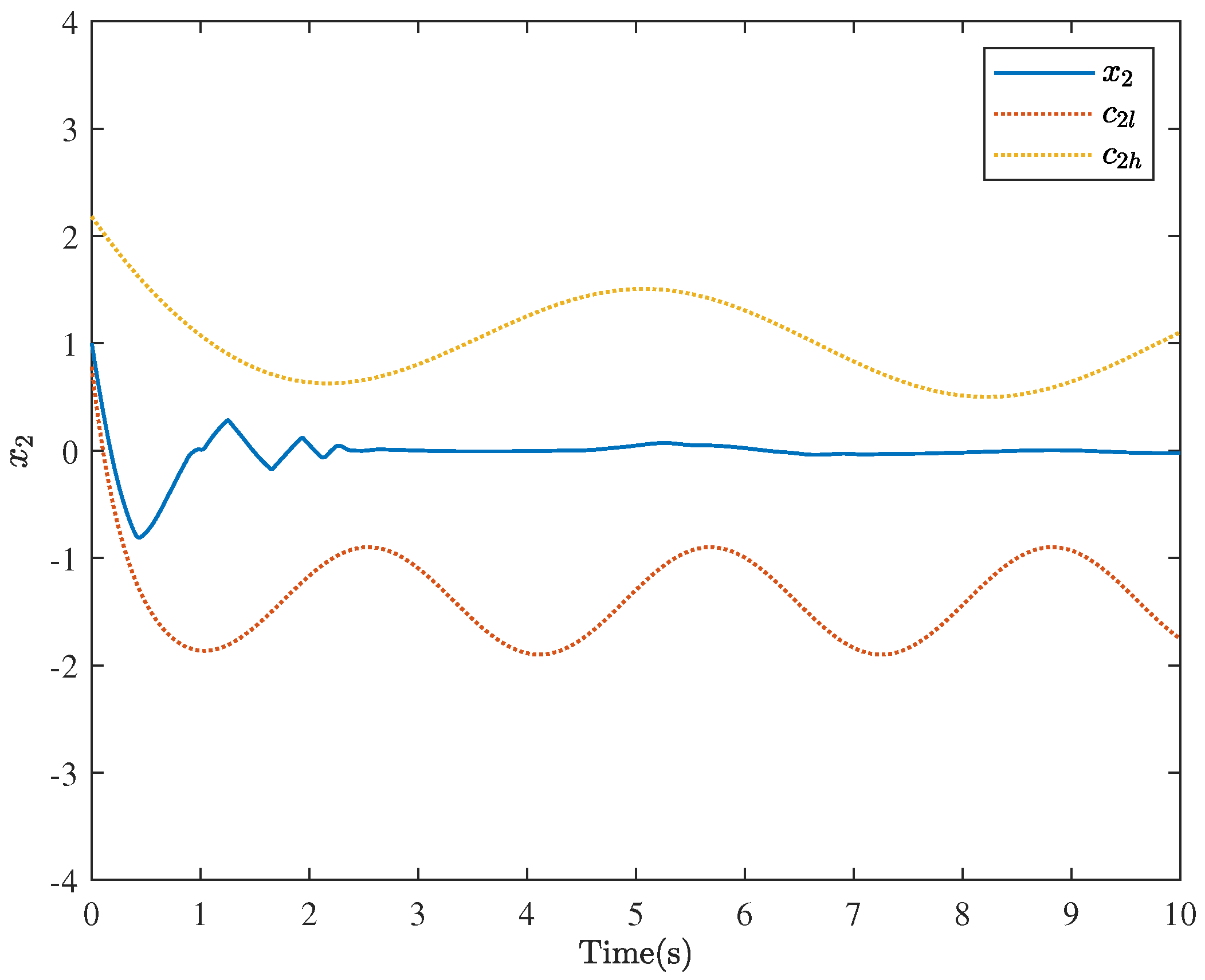
3.3. Asymmetric Time-Varying State Constraints

To guarantee that the system states always satisfy the pre-described constraints, the following uniform barrier function (UBF) [41] is designed as follows:
μ i = x i c ¯ i l x i c i l + x i c ̲ i h c i h x i , i = 2 , 3 , , n ,
where c 1 l and c 1 h are bounded constraint functions, there are constants c ¯ i l and c ̲ i h such that c i l < c ¯ i l , c ̲ i h < c 1 h , and the initial value x i ( 0 ) satisfies c i l ( 0 ) < x i ( 0 ) < c i h ( 0 ) . After transformation, Equation (16) can be converted to the following:
μ i = a i 1 x i + a i 2 ,
where a i 1 = c ¯ i l c i l + c i h c ̲ i h ( x i c i l ) ( c i h x i ) , and a i 2 = c i l c ̲ i h c ¯ i l c i h ( x i c i l ) ( c i h x i ) . Then, the following equation can be obtained:
x i = μ i a i 1 a i 3 ,
where a i 3 = a i 2 a i 1 = c i l c ̲ i h c ¯ i l c i h c ¯ i l c i l + c i h c ̲ i h . Analyzing Equation (16) shows that μ i + as x i c i h and μ i as x i c i l . Therefore, as long as μ i is guaranteed to be bounded, c i l < x i < c i h can be guaranteed. In summary, one can see that the prescribed performance problem and the state-constrained problem can be converted into a boundedness problem for μ i ( i = 1 , n ) by means of a nonlinear mapping.

4. Adaptive Control Design and Stability Analysis

The command filtering technique is employed to deal with the complexity explosion problem in the backstepping design. Before the design procedure, the subsequent coordinate change is defined as follows:
z 1 = μ 1 ,
z i = μ i α i f , i = 2 , , n ,
where α i f signifies the output of the first-order filter, which has the following form:
ε i α ˙ i f + α i f = a i 1 α i 1 , i = 2 , , n ,
where the design constant ε i is positive, α i 1 denotes the virtual control law to be designed later, and a i 1 α i 1 represents the input of the first-order filter. The filtering error representing the difference between the input and output is expressed as follows:
Y i = α i f a i 1 α i 1 , i = 2 , , n .
By utilizing Lemma 1 and Young’s inequality, we can deduce the following:
z i 3 ζ i 1 ψ i x ¯ i ( t τ i ) | z i 3 ζ i 1 | | ψ i x ¯ i ( t τ i ) | | z i 3 ζ i 1 | l = 1 i m i l x l ( t τ i ) | z i 3 ζ i 1 | m i 1 x 1 ( t τ i ) + + m i i x i ( t τ i ) 3 4 ζ i 1 4 3 z i 4 + m i 1 4 x 1 ( t τ i ) 4 + + 3 4 ζ i 1 4 3 z i 4 + m i i 4 x i ( t τ i ) 4 3 i 4 ζ i 1 4 3 z i 4 + l = 1 i m i l 4 x l ( t τ i ) 4 .
The following Lyapunov–Krasovskii function in step i ( i = 1 , , n ) should be considered to effectively compensate for the time-delay term, as follows:
V M i = e η i ( t τ i ) 4 t τ i t l = 1 i e η i s m i l 4 ( x l ( s ) ) d s ,
whose time derivative is as follows:
V ˙ M i = l = 1 i e η i τ i 4 m i l 4 ( x l ( t ) ) l = 1 i m i l 4 ( x l ( t τ i ) ) 4 η i V M i ,
where m i l is defined in Lemma 1 and η i is taken as a normal number.
The controller is designed by using the backstepping methodology and the process is as follows:
Step 1: In view of Equations (1) and (15)–(22), we have the following:
d z 1 = d μ 1 = ζ 11 d x 1 y ˙ d d t + ζ 12 d t = ζ 11 g 1 x 2 + f 1 + ψ 1 y ˙ d + ζ 12 d t + ζ 11 φ 1 T d ω = ζ 11 g 1 z 2 + Y 2 a 21 + ζ 11 g 1 α 1 + ζ 11 g 1 a 23 + f 1 + ψ 1 y ˙ d + ζ 12 d t + ζ 11 φ 1 T d ω ,
where ζ 11 = e 2 c 1 l c 1 h ( c 1 h e ) 2 ( e c 1 l ) 2 , and ζ 12 = ( c ˙ 1 l c 1 h + c 1 l c ˙ 1 h ) e ( c ˙ 1 l + c ˙ 1 h ) e 2 ( c 1 h e ) 2 ( e c 1 l ) 2 .
We construct a candidate Lyapunov function as follows:
V 1 = 1 4 z 1 4 + g 0 2 λ 1 θ ˜ 1 2 + 1 4 γ 2 Y 2 4 + V M 1 ,
where λ 1 and γ 2 are positive design constants, θ ^ 1 is an estimate of θ 1 , and the estimation error is θ ˜ 1 = θ 1 θ ^ 1 , in which θ 1 will be given later. When i = 1 , V M 1 = e η 1 ( t τ 1 ) 4 t τ 1 t e η i s m 11 4 ( x 1 ( s ) ) d s from Equation (24). Then, by taking the differential of V 1 , we have the following:
L V 1 = z 1 3 ζ 11 g 1 z 2 + Y 2 a 21 + ζ 11 g 1 α 1 + ζ 11 g 1 a 23 + f 1 + ψ 1 y ˙ d + ζ 12 + 3 2 z 1 2 ζ 11 2 Tr φ 1 T φ 1 g 0 λ 1 θ ˜ 1 θ ^ ˙ 1 + Y 2 3 γ 2 L Y 2 + e η 1 τ 1 4 m 11 4 x 1 ( t ) m 11 4 x 1 ( t τ 1 ) 4 η 1 V M 1 .
By applying Young’s inequality, we have the following:
3 2 z 1 2 ζ 11 2 Tr φ 1 T φ 1 3 4 z 1 4 ζ 11 4 φ 1 4 + 3 4 ,
z 1 3 ζ 11 g 1 z 2 a 21 3 4 ζ 11 g 1 4 3 z 1 4 + 1 4 a 21 4 z 2 4 ,
z 1 3 ζ 11 g 1 Y 2 a 21 3 4 ζ 11 g 1 4 3 z 1 4 + 1 4 a 21 4 Y 2 4 .
With Equations (21) and (22), we have the following:
d Y 2 = α ˙ 2 f d t d a 21 α 1 = Y 2 ε 2 D 2 ( · ) d t E 2 ( · ) d ω ,
where D 2 ( · ) and E 2 ( · ) are continuous functions in set i defined as follows:
D 2 ( · ) = H 1 α 1 + a 21 H 2 ,
where H 1 = a 21 x 2 ( g 2 x 3 + f 2 + ψ 2 ) + 2 a 21 2 x 2 2 Tr { φ 2 T φ 2 } + a 21 c 2 l c ˙ 2 l + a 21 c 2 h c ˙ 2 h + a 21 c ˙ 2 l c ¨ 2 l + a 21 c ˙ 2 h c ¨ 2 h , H 2 = α 1 x 1 ( g 1 x 2 + f 1 + ψ 1 ) + 2 α 1 2 x 1 2 Tr { φ 1 T φ 1 } + α 1 c 1 l c ˙ 1 l + α 1 c 1 h c ˙ 1 h + α 1 c ˙ 1 l c ¨ 1 l + α 1 c ˙ 1 h c ¨ 1 h + α 1 y d y ˙ d + α 1 y ˙ d y ¨ d + α 1 θ ^ 1 θ ^ ˙ 1 , and E 2 ( · ) = a 21 x 2 φ 2 α 1 + α 1 x 1 a 21 φ 1 . Define the compacts Ω V = { i = 1 n 1 4 z i 4 + i = 1 n g 0 2 λ i θ ˜ i 2 + i = 1 n 1 1 4 λ i + 1 Y i + 1 4 Q ¯ } , Ω i j = { [ c i j , c i j ˙ , c i j ¨ ] T : c i j 2 + c i j ˙ 2 + c i j ¨ 2 Q , i = 1 , , n , j = l , h } , and Ω d = { [ y d , y d ˙ , y d ¨ ] T : y d 2 + y d ˙ 2 + y d ¨ 2 Q ̲ } , in which Q ¯ , Q and Q ̲ are positive constants. There exist positive constants D ¯ 2 and E ¯ 2 in the compacts Ω V × Ω d × Ω i j satisfying D 2     D ¯ 2 and E 2     E ¯ 2 , respectively. Then, we have the following:
Y 2 3 L Y 2 = Y 2 4 ϵ 2 Y 2 3 D 2 + 3 2 Y 2 2 Tr E 2 T E 2 .
According to Young’s inequality, we have the following: Y 2 3 D 2 3 4 Y 2 4 + 1 4 D ¯ 2 4 , and 3 2 Y 2 3 Tr { E 2 T E 2 } 3 4 Y 2 4 + 3 4 E ¯ 2 4 . Then, Equation (34) can be modified into the following:
Y 2 3 L Y 2 3 2 1 ϵ 2 Y 2 4 + O 2 ,
where O 2 = ( 1 / 4 ) D ¯ 2 4 + ( 3 / 4 ) E ¯ 2 4 is a positive constant. By inserting Equations (29)–(31) and (35) into (28), we obtain the following:
L V 1 z 1 3 ζ 11 g 1 α 1 + F 1 ( Z 1 ) 3 4 z 1 4 + 3 4 g 0 λ 1 θ ˜ 1 θ ^ ˙ 1 K 2 Y 2 4 + 1 4 a 21 4 z 2 4 + U 1 η 1 V M 1 ,
where F 1 ( Z 1 ) = ζ 11 ( g 1 a 23 + f 1 y ˙ d ) + ζ 12 + 3 4 z 1 ζ 11 φ 1 4 + 3 4 z 1 + 3 2 ( ζ 11 g 1 ) 4 3 z 1 + 3 4 ( ζ 11 ) 4 3 z 1 , K 2 = 1 γ 2 ( 1 ϵ 2 3 2 ) 1 4 a 21 4 , and U 1 = 1 γ 2 O 2 + e η 1 τ 1 4 m 11 4 ( x 1 ( t ) ) . Selecting the appropriate design parameters γ 2 and ϵ 2 can make K 2 > 0 .
Based on Lemma 2, the RBF neural network W 1 * T Ξ 1 ( Z 1 ) is used to approximate F 1 ( Z 1 ) , i.e., there is F 1 ( Z 1 ) = W 1 * T Ξ 1 ( Z 1 ) + δ 1 ( Z 1 ) . According to the nature of the neural network basis function, it is known that Ξ 1 ( Z 1 ) T Ξ 1 ( Z 1 ) l 1 , in which l 1 denotes the dimension of Ξ 1 ( Z 1 ) . Since the dimension l i of the basis function and the optimal weight vector W i * T cannot be determined directly, the adaptive parameter is defined as follows:
θ i = l i W i * T 2 g 0 1 , i = 1 , , n 1 ,
where the estimate of θ i is θ ^ i and the estimation error is θ ˜ i = θ i θ ^ i . Based on Lemma 3, we can obtain the following:
z 1 3 F 1 = z 1 3 W 1 * T Ξ 1 ( Z 1 ) + δ 1 ( Z 1 ) l 1 2 a 1 2 z 1 6 W 1 * T 2 + a 1 2 2 + 3 4 z 1 4 + Δ 1 4 4 g 0 2 a 1 2 z 1 6 θ 1 + a 1 2 2 + 3 4 z 1 4 + Δ 1 4 4 ,
where a 1 is a positive design constant. Along with Equation (38), Equation (36) can be rewritten as follows:
L V 1 g 0 2 a 1 2 z 1 6 θ 1 + a 1 2 2 + Δ 1 4 4 + z 1 3 ζ 11 g 1 α 1 + 3 4 g 0 λ 1 θ ˜ 1 θ ^ ˙ 1 K 2 Y 2 4 + 1 4 a 21 4 z 2 4 + U 1 η 1 V M 1 .
The virtual controller and adaptive law of the first subsystem are designed as follows:
α 1 = 1 ζ 11 c 1 z 1 1 2 a 1 2 z 1 3 θ ^ 1 ,
θ ^ ˙ 1 = λ 1 2 a 1 2 z 1 6 σ 1 θ ^ 1 ,
where c 1 , σ 1 , and λ 1 denote positive design parameters.
By substituting Equations (40) and (41) into (39), and using inequality g 0 σ 1 λ 1 θ ˜ 1 θ ^ 1 g 0 σ 1 2 λ 1 θ ˜ 1 2 + g 0 σ 1 2 λ 1 θ 1 2 , we obtain the following:
L V 1 c 1 g 0 z 1 4 g 0 σ 1 2 λ 1 θ ˜ 1 2 K 2 Y 2 4 η 1 V M 1 + 1 4 a 21 4 z 2 4 + Γ 1 ,
where Γ 1 = g 0 σ 1 2 λ 1 θ 1 2 + a 1 2 2 + Δ 1 4 4 + 3 4 + U 1 .
Step i  ( 2 i n 1 ) : Akin to Step 1, by means of Equations (1) and (16)–(22), we have the following:
d z i = ζ i 1 g i z i + 1 + Y i + 1 a i + 1 , 1 + ζ i 1 g i α i + ζ i 1 g i a i + 1 , 3 + f i + ψ i + ζ i 2 α ˙ i f d t + Φ i T d ω ,
where ζ i 1 = c ¯ i l c i l ( x i c i l ) 2 + c i h c ̲ i h ( c i h x i ) 2 , ζ i 2 = ( x i c ¯ i l ) c ˙ i l ( x i c i l ) 2 ( x i c ̲ i h ) c ˙ i h ( c i h x i ) 2 , and Φ i = ζ i 1 φ i j = 1 i 1 α i 1 x j ζ j 1 φ j .
We construct a candidate Lyapunov function as follows:
V i = V i 1 + 1 4 z i 4 + g 0 2 λ i θ ˜ i 2 + 1 4 γ i + 1 Y i + 1 4 + V M i ,
where λ i and γ i + 1 are positive design constants, g 0 is an unknown parameter, θ ^ i is an estimate of θ i , the estimation error is θ ˜ i = θ i θ ^ i , and θ i is given by Equation (37).
Similar to Equation (28), it is easy to obtain the following:
L V i = L V i 1 + z i 3 ζ i 1 g i z i + 1 + Y i + 1 a i + 1 , 1 + ζ i 1 g i α i + ζ i 1 g i a i + 1 , 3 + f i + ψ i + ζ i 2 α ˙ i f + 3 2 z i 2 Tr Φ i T Φ i g 0 λ i θ ˜ i θ ^ ˙ i + Y i + 1 3 γ i + 1 L Y i + 1 + l = 1 i e η i τ i 4 m i l 4 x l ( t ) l = 1 i m i l 4 x l ( t τ i ) 4 η i V M i .
Then, by using Young’s inequality, we have the following:
z i 3 ζ i 1 ψ i x ¯ i ( t τ i ) 3 i 4 ζ i 1 4 3 z i 4 + l = 1 i m i l 4 x l ( t τ i ) 4 ,
3 2 z i 2 Tr Φ i T Φ i 3 4 z i 4 Φ i T 4 + 3 4 ,
z i 3 ζ i 1 g i z i + 1 a i + 1 , 1 3 4 ζ i 1 g i 4 3 z i 4 + 1 4 a i + 1 , 1 4 z i + 1 4 ,
z i 3 ζ i + 1 , 1 g i Y i + 1 a i + 1 , 1 3 4 ζ i 1 g i 4 3 z i 4 + 1 4 a i + 1 , 1 4 Y i + 1 4 .
Similar to the analysis method in step 1, we have the following:
Y i + 1 3 L Y i + 1 3 2 1 ϵ i + 1 Y i + 1 4 + O i + 1 ,
where O i + 1 = ( 1 / 4 ) D ¯ i + 1 4 + ( 3 / 4 ) E ¯ i + 1 4 is a positive constant.
By incorporating Equations (46)–(50) into (45), we have the following:
L V i L V i 1 + z i 3 ζ i 1 g i α i + F i ( Z i ) 1 4 a i , 1 4 z i 4 3 4 z i 4 + 3 4 g 0 λ i θ ˜ i θ ^ ˙ i K i + 1 Y i + 1 4 + 1 4 a i + 1 , 1 4 z i + 1 4 + U i η i V M i ,
where F i ( Z i ) = ζ i 1 ( g i a i + 1 , 3 + f i ) + ζ i 2 α ˙ i f + 3 4 z i Φ i T 4 + 3 4 z i + 3 2 ( ζ i 1 g i ) 4 3 z i + 3 i 4 ( ζ i 1 ) 4 3 z i + 1 4 a i , 1 4 z i , K i + 1 = 1 γ i + 1 ( 1 ϵ i + 1 3 2 ) 1 4 a i + 1 , 1 4 , and U i = 1 γ i + 1 O i + 1 + l = 1 i e η i τ i 4 m i l 4 ( x l ( t ) ) . Selecting the appropriate design parameters γ i + 1 and ϵ i + 1 can make K i + 1 > 0 .
Based on Lemma 2, the RBF neural network W i * T Ξ i ( Z i ) is used to approximate F i ( Z i ) , i.e., there is F i ( Z i ) = W i * T Ξ i ( Z i ) + δ i ( Z i ) . Similar to Lemma 3, the following inequality holds: z i 3 F i g 0 2 a i 2 z i 6 θ i + a i 2 2 + 3 4 z i 4 + Δ i 4 4 , where a i is a positive design constant. Substituting this inequality into Equation (51) yields the following:
L V i L V i 1 + g 0 2 a i 2 z i 6 θ i + a i 2 2 + Δ i 4 4 + z i 3 ζ i 1 g i α i 1 4 a i , 1 4 z i 4 + 3 4 g 0 λ i θ ˜ i θ ^ ˙ i K i + 1 Y i + 1 4 + 1 4 a i + 1 , 1 4 z i + 1 4 + U i η i V M i .
The virtual controller and adaptive law of the ith subsystem are designed as follows:
α i = 1 ζ i 1 c i z i 1 2 a i 2 z i 3 θ ^ i ,
θ ^ ˙ i = λ i 2 a i 2 z i 6 σ i θ ^ i ,
where c i , σ i , and λ i denote positive design parameters.
By substituting Equations (53) and (54) into (52) and using inequality g 0 σ i λ i θ ˜ i θ ^ i g 0 σ i 2 λ i θ ˜ i 2 + g 0 σ i 2 λ i θ i 2 , we obtain the following:
L V i i = 1 n 1 c i g 0 z i 4 i = 1 n 1 g 0 σ i 2 λ i θ ˜ i 2 i = 1 n 1 K i + 1 Y i + 1 4 i = 1 n 1 η i V M i + 1 4 a i + 1 , 1 4 z i + 1 4 + i = 1 n 1 Γ i ,
where Γ i = g 0 σ i 2 λ i θ i 2 + a i 2 2 + Δ i 4 4 + 3 4 + U i .
Step n: Based on Equations (1) and (16)–(22), we have the following:
d z n = ζ n 1 g n k v v + q ( v ) + ζ n 1 f n + ψ n + ζ n 2 α ˙ n f d t + Φ n T d ω ,
where ζ n 1 = c ¯ n l c n l ( x n c n l ) 2 + c n h c ̲ n h ( c n h x n ) 2 , ζ n 2 = ( x n c ¯ n l ) c ˙ n l ( x n c n l ) 2 ( x n c ̲ n h ) c ˙ n h ( c n h x n ) 2 , and Φ n = ζ n 1 φ n j = 1 n 1 α n 1 x j ζ j 1 φ j . We take into account the Lyapunov function provided below:
V n = V n 1 + 1 4 z n 4 + g 0 k m 2 λ n θ ˜ n 2 + V M n ,
where λ n is a positive design constant and the definition of the normal number k m can be seen in Section 3.1; θ n is given later.
Similar to Equation (28), we obtain the following:
L V n = L V n 1 + z n 3 ζ n 1 g n k v v + q ( v ) + ζ n 1 f n + ψ n + ζ n 2 α ˙ n f + 3 2 z n 2 Tr Φ n T Φ n g 0 k m λ n θ ˜ n θ ^ ˙ n + l = 1 n e η n τ n 4 m n l 4 x l ( t ) l = 1 n m n l 4 x l ( t τ n ) 4 η n V M n .
Then, by employing Young’s inequality, we have the following:
z n 3 ζ n 1 ψ n x ¯ n ( t τ n ) 3 n 4 ζ n 1 4 3 z n 4 + l = 1 n m n l 4 x l ( t τ n ) 4 ,
3 2 z n 2 Tr Φ n T Φ n 3 4 z n 4 Φ n T 4 + 3 4 .
By substituting Equations (59) and (60) into (58), we have the following:
L V n L V n 1 + z n 3 [ ζ n 1 g n k v v + q ( v ) + ζ n 1 f n + ζ n 2 α ˙ n f + 3 4 z n Φ n T 4 + 3 4 z n + 3 n 4 ζ n 1 4 3 z n ] 3 4 z n 4 + 3 4 g 0 k m λ n θ ˜ n θ ^ ˙ n + U n η n V M n ,
where F n ( Z n ) = ζ n 1 g n q ( v ) + ζ n 1 f n + ζ n 2 α ˙ n f + 3 4 z n Φ n T 4 + 3 4 z n + 3 n 4 ( ζ n 1 ) 4 3 z n + 1 4 a n 1 4 z n , and U n = l = 1 n e η n τ n 4 m n l 4 ( x l ( t ) ) .
Based on Lemma 2, the RBF neural network W n * T Ξ n ( Z n ) is used to approximate F n ( Z n ) , i.e., there is F n ( Z n ) = W n * T Ξ n ( Z n ) + δ n ( Z n ) . As in Equation (37), we define the adaptive parameter as θ n = l n W n * T 2 g 0 1 k m 1 . Similar to Lemma 3, the following inequality holds: z n 3 F n g 0 k m 2 a n 2 z n 6 θ n + a n 2 2 + 3 4 z n 4 + Δ n 4 4 , where a n is a positive design constant. Substituting this inequality into Equation (61) yields the following:
L V n i = 1 n 1 c i g 0 z i 4 i = 1 n 1 g 0 σ i 2 λ i θ ˜ i 2 i = 1 n 1 K i + 1 Y i + 1 4 i = 1 n 1 η i V M i + i = 1 n 1 Γ i + z n 3 ( ζ n 1 g n k v v ) + g 0 k m 2 a n 2 z n 6 θ n + a n 2 2 + Δ n 4 4 + 3 4 g 0 k m λ n θ ˜ n θ ^ ˙ n + U n η n V M n .
The ideal controller and adaptive law of the nth subsystem are designed as follows:
v = 1 ζ n 1 c ¯ n z n 1 2 a n 2 z n 3 θ ^ n ,
θ ^ ˙ n = λ n 2 a n 2 z n 6 σ ¯ n θ ^ n ,
where c ¯ n , σ i , a n , and λ ¯ n denote positive design parameters.
By substituting Equations (63) and (64) into (62) and using inequality g 0 σ n λ n θ ˜ n θ ^ n g 0 σ n 2 λ n θ ˜ n 2 + g 0 σ n 2 λ n θ n 2 , we obtain the following:
L V n i = 1 n c i g 0 z i 4 i = 1 n g 0 σ i 2 λ i θ ˜ i 2 i = 1 n 1 K i + 1 Y i + 1 4 i = 1 n η i V M i + i = 1 n Γ i ,
where Γ n = g 0 k m σ ¯ n 2 λ n θ n 2 + a n 2 2 + Δ n 4 4 + 3 4 + U n , c n = k m c ¯ n , and σ n = k m σ ¯ n .
The backstepping technique is illustrated in Figure 1 for better clarity.
Remark 3. 
The backstepping technique is a classic controller design method proposed by [51]; it has been widely used. Its basic idea is to transform the controller design problem of a high-order system into the design of virtual controllers for lower-order systems. In the design of each low-order subsystem, an intermediate virtual control variable is introduced to stabilize the subsystem and compensate for the influence brought by the residual terms of the previous subsystem. Its design direction is opposite to the controller’s control direction.
Theorem 1 is a high generalization of the main results of this paper.
Theorem 1. 
In the case of system (1) satisfying Assumptions 1 and 2, and when the initial values of the system state variables meet the constraints, the virtual control laws (40), (53), and (63), as well as the adaptive laws (41), (54), and (64), are used in order to achieve the following: (1) all the signals of the closed-loop system are bounded. (2) The system states always satisfy the pre-described constraints, even if the signs of the constraint boundary functions change. (3) The output y can track the reference signal y d before a specified time T f , and the tracking error e satisfies the preset performance constraint.
Proof. 
In accordance with the process employed in designing the controller, the following inequality can be derived:
L V n i = 1 n c i g 0 z i 4 i = 1 n g 0 σ i 2 λ i θ ˜ i 2 i = 1 n 1 K i + 1 Y i + 1 4 i = 1 n η i V M i + i = 1 n Γ i C V n + D ,
where C = min { 4 c i g 0 , σ i , 4 γ i + 1 K i + 1 , η i } , i = 1 , , n , and D = i = 1 n Γ i . Based on reference [52], we have the following:
d ( E [ V n ] ) d t = E [ L V n ] C E [ V n ] + D .
If E [ V n ] = β and C > D / β , then d ( E [ V n ] ) d t 0 . Furthermore, it has E [ V n ( t ) ] β when E [ V n ( 0 ) ] β for all t 0 . Availing oneself of Lemma 4, we have the following:
0 E [ V n ( t ) ] V n ( 0 ) e C t + D C , t 0 ,
which means that E [ V n ( t ) ] D C , while t . According to the above analysis, it is easy to conclude that the signals θ ˜ i , Y i , and z i are bounded. Then, the following results are allowed to be derived.
1. All the signals belonging to the closed-loop system are bounded according to the following analysis. μ 1 is bounded through the boundedness of z 1 , which means that x 1 , and ζ 11 are bounded. Based on Equation (40), it indicates that α 1 is bounded, then according to Equation (22), α 2 f is also bounded. From Equation (20), we can conclude that μ 2 is bounded, which implies that both x 2 and ζ 21 are bounded. According to Equation (53), it is indicated that α 2 is bounded; thus, it follows from Equation (22) that α 3 f is bounded. By proceeding in this manner, z i , x i , Y i , μ i , α i , and v are all bounded.
2. The system states always satisfy the pre-described constraints. That is, from Equation (16), it follows that each x i is within the asymmetric time-varying constraint range ( c i l , c i h ) due to the boundedness of μ i .
3. The output y can track the reference signal y d before the specified time T f , and the tracking error e satisfies the preset performance constraint. In other words, according to the analysis around Equation (15), c 1 l < e < c 1 h is guaranteed because μ 1 is bounded.
The proof is completed. □

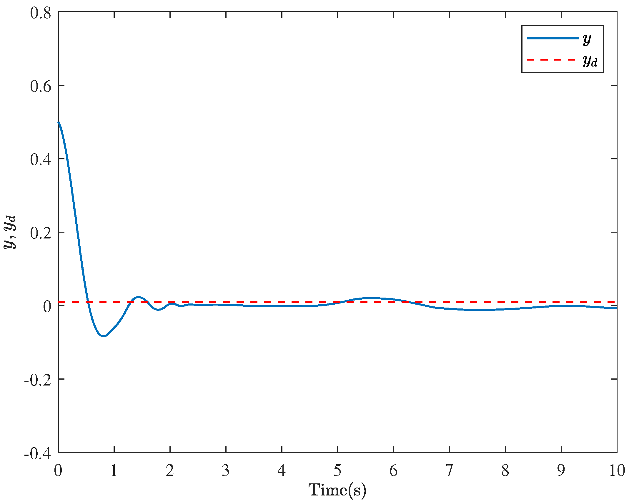
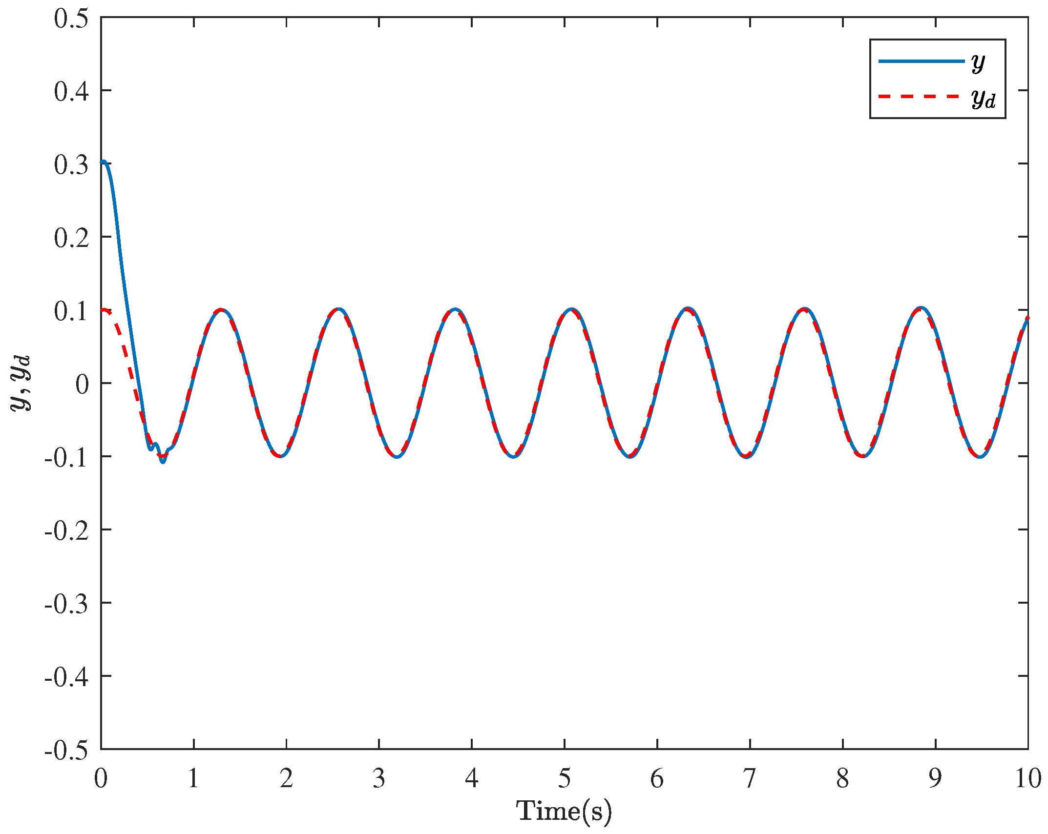
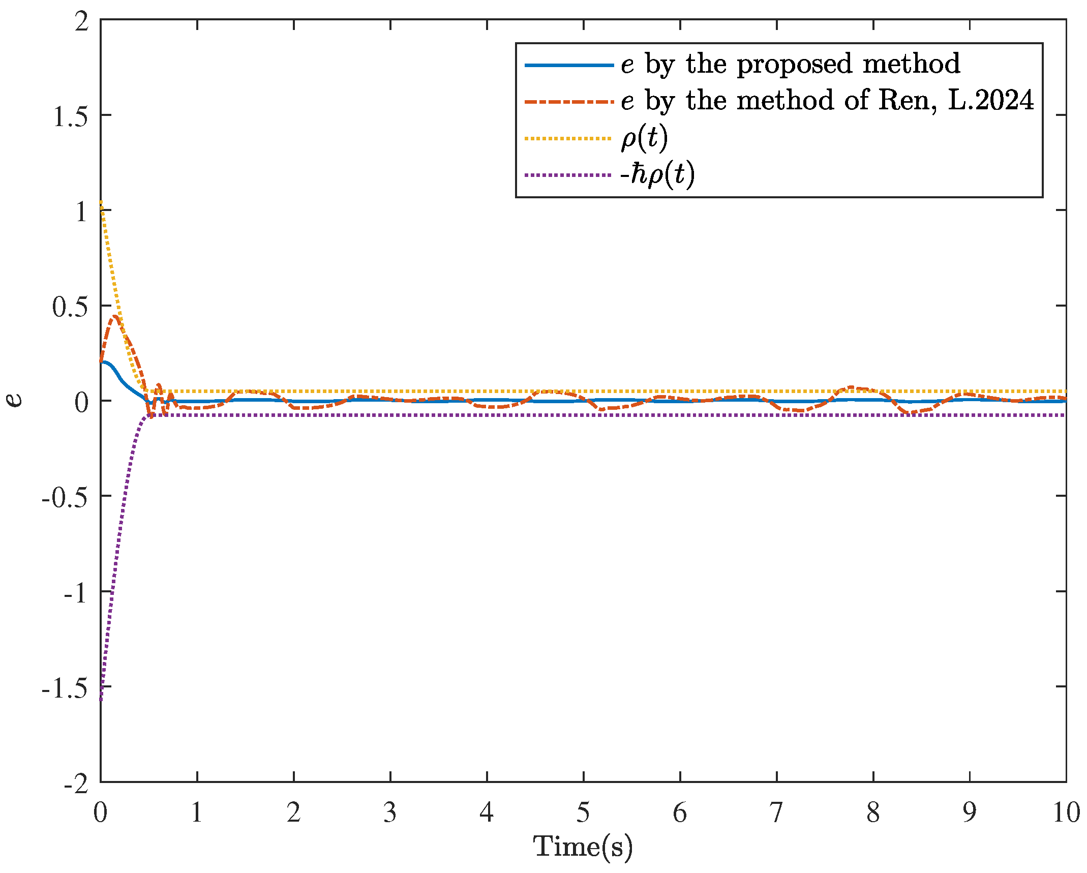
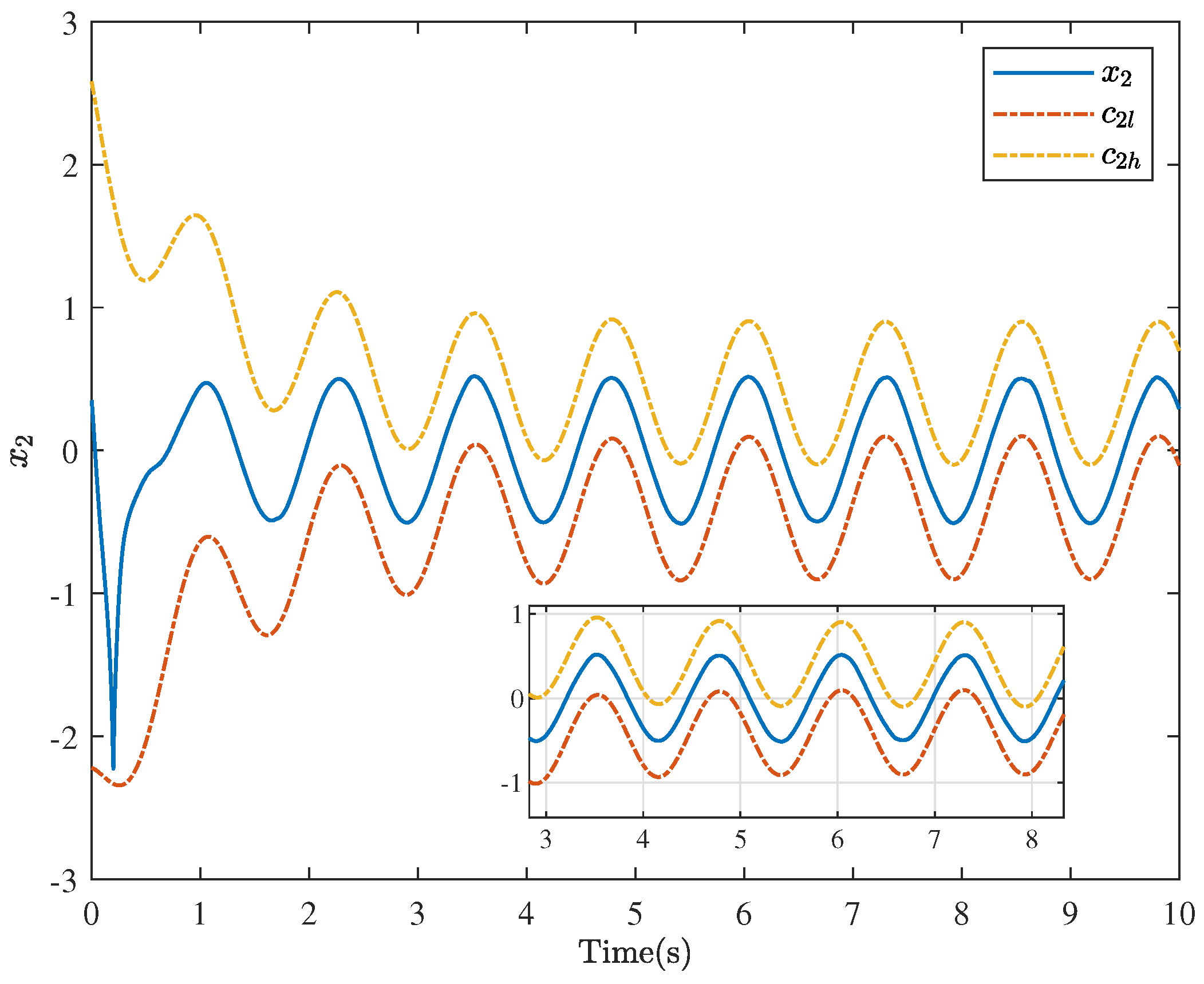
5. Simulation Examples

Example 1. 
In order to verify the effectiveness of the proposed control scheme, the two-stage chemical reactor with delayed recycle streams (shown in Figure 2) is given [42,43,44].
Encouraged by [42,43,44], the two-stage chemical reactor can be depicted by the following structure:
d x 1 = 1 R B V A x 2 1 G A x 1 + ψ 1 x 1 ( t τ 1 ) d t 0.01 x 1 d ω , d x 2 = F V B u ( v ) 1 G B x 2 C B x 2 + ψ 2 x ¯ 2 ( t τ 2 ) d t 0.1 x 2 d ω , y = x 1 ,
where x 1 and x 2 denote the concentrations of the produce streams from reactors A and B. A and B are both time-delay systems, and there are time-delay phenomena in the recycling of concentrations, which are caused by the feed rate, reaction volume, reactor residence time, and so on. The time delay in the recycling of concentrations is as follows: ψ 1 ( x 1 ( t τ 1 ) ) = 1 G A x 1 ( t τ 1 ) , and ψ 2 ( x ¯ 2 ( t τ 2 ) ) = R A V B x 1 ( t τ 2 ) R B V B x 2 ( t τ 2 ) + 0.1 x 2 2 ( t τ 2 ) , where τ 1 = τ 2 = 0.5 . The reference trajectory y d is selected as y d = 0.01 ; the practical significance and values of the system parameters are shown in Table 1. Additional information can be seen in [46].
Remark 4. 
By monitoring the reactant concentrations, the controller is designed to ensure the entire reaction system can operate safely and efficiently. Restricting the range of reactant concentrations in advance can help prevent excessively high concentrations that may cause violent reactions or accidents, as well as low concentrations that lead to low reaction efficiency [11,12].
During the simulation, the state constraint boundary functions are selected as c 2 l = 0.5 cos ( 2 t + 1.2 ) + 2 e 4 t 1.4 and c 2 h = 0.5 cos ( t + 1.2 ) + e t + 1 , respectively. The initial states of the system are chosen as [ x 1 ( 0 ) , x 2 ( 0 ) , θ ^ 1 ( 0 ) , θ ^ 2 ( 0 ) ] T = [ 0.5 , 1 , 0 , 1 ] T . The other design parameters are chosen as c ¯ 2 l = 10 , c ̲ 2 h = 10 , c 1 = 9 , c 2 = 2 , a 1 = 10 , a 2 = 30 , λ 1 = 0.001 , λ 2 = 0.001 , σ 1 = 0.3 , σ 2 = 0.1 , u P = 20 , u S = 20 , ϵ 2 = 0.01 , ϱ 0 = 1 , T f = 1.5 , ϱ T f = 0.05 and = 1.5 .
The simulation results are presented in Figure 3, Figure 4, Figure 5 and Figure 6. The motion trajectory and tracking situations of the system output are illustrated in Figure 3. Figure 4 shows the results with tracking errors satisfying the performance constraint. It can be seen from Figure 3 and Figure 4 that the system output y can track the reference signal y d before T f = 1.5 s, and the tracking accuracy falls within the range of (−0.075, 0.05). Figure 4 also gives the tracking error under the action of the control method in Reference [46]. Compared with this method, the method proposed in this paper can guarantee that the tracking error always satisfies the prescribed performance constraints, which can effectively increase the tracking speed and substantially improve the tracking accuracy. Additionally, the association between the desired control law v and the saturated actuator u is depicted in Figure 5. It is noticeable that the controller can achieve the control objectives despite being affected by saturation. Figure 6 gives the changing curve of the system state x 2 , and it is evident that the state x 2 always stays within the constraint range. It also indicates that the signs of the constraint boundary functions c 2 l and c 2 h are variable, that is, neither constantly positive nor constantly negative, which means that the limitation is broken. In summary, the simulation results demonstrate the feasibility and superiority of the control method in this paper.
Example 2. 
To demonstrate the effectiveness of the proposed approach, we carry out the following numerical example, which is given in [41]. Consider the following nonlinear stochastic time-delay system:
d x 1 = 2 x 2 + 0.01 x 1 2 0.5 x 1 ( t τ 1 ) d t + x 2 3 d ω , d x 2 = 1.5 u + x 1 x 2 0.1 x 1 ( t τ 2 ) + 0.5 x 2 ( t τ 2 ) d t + 0.2 x 1 s i n ( x 2 ) d ω , y = x 1 .
The reference trajectory y d is selected as y d = 0.1 sin ( 5 t + 1.4 ) . During the simulation, the state constraints boundary functions are selected as c 2 l = 0.5 cos ( 5 t + 1.2 ) 2 e t 0.4 and c 2 h = 0.5 cos ( 5 t + 1.2 ) + 2 e t + 0.4 , respectively. The initial states of the system are chosen as x 1 ( 0 ) = 0.3 , x 2 ( 0 ) = 0.35 , θ ^ 1 ( 0 ) = 0 , θ ^ 2 ( 0 ) = 1 . The other design parameters are chosen as c ¯ 2 l = 5 , c ̲ 2 h = 5 , c 1 = 0.1 , c 2 = 0.1 , a 1 = 2 , a 2 = 2 , λ 1 = 1 , λ 2 = 1 , σ 1 = 0.3 , σ 2 = 0.1 , u P = 10 , u S = 10 , ϵ 2 = 0.01 , ϱ 0 = 1 , T f = 0.6 , ϱ T f = 0.05 and = 1.5 .
The simulation results are presented in Figure 7, Figure 8, Figure 9 and Figure 10. In addition, to further illustrate the effect of different design methods on the dynamic performance of tracking error, comparisons between the proposed method and the method described in [41] are listed in Table 2.
In Table 2, TMTE is the maximum transient error, and TMSSE is the maximum steady-state error. TECT is the error convergence time. When t TECT, | e | ϱ T f . It can be observed from Figure 8 and Table 2 that (1) the tracking error always satisfies the performance constraints; (2) by using the proposed method, the tracking accuracy falls within the range (−0.005, 0.005) before the finite time T f = 0.6 and will always be within it later; and (3) by using the proposed method, the tracking error achieves good transient and steady-state tracking performance.
The motion trajectory and tracking situations of the system output are illustrated in Figure 7. Compared to [41], our article offers some advantages. As shown in Figure 8, the method proposed in this paper can guarantee that the tracking error always satisfies the prescribed performance constraints, which can effectively increase the tracking speed and substantially improve the tracking accuracy. As depicted in Figure 9, it is noticeable that the controller can achieve the control objectives despite being affected by saturation. Additionally, Figure 10 gives the changing curve of the system state x 2 , and it is evident that the state x 2 always stays within the constraint range. Different from [30,31,32], it can be observed that the signs of the constraint boundary functions c 2 l and c 2 h are variable, that is, neither constantly positive nor constantly negative. In summary, the simulation results demonstrate the feasibility and superiority of the control method in this paper.

6. Conclusions

This paper proposes a prescribed performance tracking control scheme for a category of stochastic time-delay nonlinear systems. The control input of this system is subject to a saturation constraint, the system state variables must satisfy asymmetric time-varying constraints, and the tracking error should meet the prescribed performance constraint. First, a suitable nonlinear function was selected to approximate the saturation function to solve the non-conductivity problem caused by the saturated input. A nonlinear mapping technique was adopted to transform the constrained problem into a bounded convergence problem, thereby solving the problem of the system state variables and the tracking error subject to the constraints. Additionally, to eliminate the unfavorable effects of the time delay, a suitable Lyapunov–Krasovskii function was introduced to compensate for the time delay term. Based on this, the error feedback controller was designed by combining the backstepping technique, dynamic surface technique, neural network approximation technique, and adaptive control method. Both theoretical analysis and simulation results indicate that the designed controller not only ensures that all signals of the closed-loop system are bounded but also guarantees that the system states always remain within the prescribed range. The tracking error can converge to the preset accuracy range within a preset time, which meets the prescribed performance requirements. Our future study will further explore methods to reduce transmission from the controller to the actuator.

Author Contributions

Conceptualization, R.C.; software, M.Z.; methodology, R.C. and M.Z.; resources, M.Z.; validation, M.Z., R.C. and Y.W.; writing—review and editing, R.C. and Y.W.; formal analysis, R.C.; data curation, M.Z.; supervision, M.Z.; writing—original draft preparation, M.Z. All authors have read and agreed to the published version of the manuscript.

Funding

This research received funding from the Fundamental Research Program of Shanxi Province under grant number 202303021221063.

Data Availability Statement

Data sharing does not apply to this article, as no datasets were generated or analyzed during the current study.

Acknowledgments

The authors wholeheartedly express their appreciation for the editors’ and reviewers’ kind attention and valuable comments, which have greatly contributed to this paper.

Conflicts of Interest

The authors declare no conflicts of interest.

References

  1. AlNemer, G.; Hosny, M.; Udhayakumar, R.; Elshenhab, A.M. Existence and hyers–ulam stability of stochastic delay systems governed by the rosenblatt process. Mathematics 2024, 12, 1729. [Google Scholar] [CrossRef]
  2. Zhu, Q.X. Stability analysis of stochastic delay differential equations with Lévy noise. J. Frankl. Inst. 2018, 118, 62–68. [Google Scholar] [CrossRef]
  3. Chen, H.; Shi, P.; Lim, C. Stability analysis for nonautonomous impulsive hybrid stochastic delay systems. Syst. Control. Lett. 2024, 187, 105785. [Google Scholar] [CrossRef]
  4. Min, H.; Xu, S.; Zhang, B.; Ma, Q. Globally adaptive control for stochastic nonlinear time-delay systems with perturbations and its application. Automatica 2019, 102, 105–110. [Google Scholar] [CrossRef]
  5. Fan, L.; Zhu, Q.; Zheng, W. Stability analysis of switched stochastic nonlinear systems with state-dependent delay. IEEE Trans. Autom. Control 2024, 69, 2567–2574. [Google Scholar] [CrossRef]
  6. Sun, S.; Zhang, H.; Zhang, J.; Yu, L.; Sun, J. Multiple delay-dependent robust H finite-time filtering for uncertain itô stochastic takagi–sugeno fuzzy semi-markovian jump systems with state constraints. IEEE Trans. Fuzzy Syst. 2020, 30, 321–331. [Google Scholar] [CrossRef]
  7. Ding, K.; Zhu, Q.; Zheng, W. Disturbance-observer-based finite-time antidisturbance control for Markov switched descriptor systems with multi-disturbances and intermittent measurements. IEEE Trans. Circuits Syst. I Regul. Pap. 2023, 70, 2968–2981. [Google Scholar] [CrossRef]
  8. Ding, L.; Li, S.; Liu, Y.; Gao, H.; Chen, C.; Deng, Z. Adaptive neural network-based tracking control for full-state constrained wheeled mobile robotic system. IEEE Trans. Syst. Man Cybern. Syst. 2017, 47, 2410–2419. [Google Scholar] [CrossRef]
  9. Gao, H.; Song, X.; Ding, L.; Deng, Z. Adaptive tracking control of nonholonomic systems based on feedback error learning. Int. J. Robot. Autom. 2013, 28, 371–378. [Google Scholar] [CrossRef]
  10. Li, Z.; Li, J.; Kang, Y. Adaptive robust coordinated control of multiple mobile manipulators interacting with rigid environments. Automatica 2010, 46, 2028–2034. [Google Scholar] [CrossRef]
  11. Jakobsen, H.A. Chemical Reactor Modeling, Multiphase Reactive Flows; Springer: Cham, Switzerland, 2018. [Google Scholar]
  12. Mhaskar, P.; Kennedy, A.B. Robust model predictive control of nonlinear process systems: Handling rate constraints. Chem. Eng. Sci. 2008, 63, 366–375. [Google Scholar] [CrossRef]
  13. Tee, K.; Ge, S.; Tay, E. Barrier Lyapunov functions for the control of output-constrained nonlinear systems. Automatica 2009, 45, 918–927. [Google Scholar] [CrossRef]
  14. Ren, B.; Ge, S.; Tee, K.; Lee, T. Adaptive neural control for output feedback nonlinear systems using a barrier Lyapunov function. IEEE Trans. Neural Netw. 2010, 21, 1339–1345. [Google Scholar] [PubMed]
  15. Guo, T.; Wu, X. Backstepping control for output-constrained nonlinear systems based on nonlinear mapping. Neural Comput. Appl. 2014, 25, 1665–1674. [Google Scholar] [CrossRef]
  16. Liu, Y.; Ma, L.; Liu, L.; Tong, S.; Chen, C.P. Adaptive neural network learning controller design for a class of nonlinear systems with time-varying state constraints. IEEE Trans. Neural Netw. Learn. Syst. 2020, 31, 66–75. [Google Scholar] [CrossRef]
  17. Liu, X.; Gao, C.; Wang, H.; Wu, L.; Yang, Y. Adaptive neural tracking control of full-state constrained nonstrict-feedback time-delay systems with input saturation. Int. J. Control. Autom. Syst. 2020, 18, 2048–2060. [Google Scholar] [CrossRef]
  18. Fang, L.; Ma, L.; Ding, S.; Park, J. Finite-time stabilization of high-order stochastic nonlinear systems with asymmetric output constraints. IEEE Trans. Syst. Man Cybern. Syst. 2021, 51, 7201–7213. [Google Scholar] [CrossRef]
  19. Shu, Y. BLF-based neural dynamic surface control for stochastic nonlinear systems with time delays and full-state constraints. Int. J. Control 2024, 97, 982–998. [Google Scholar] [CrossRef]
  20. Vo, A.; Truong, T.; Kang, H.J.; Le, T. A fixed-time sliding mode control for uncertain magnetic levitation systems with prescribed performance and anti-saturation input. Eng. Appl. Artif. Intell. 2024, 133, 108373. [Google Scholar] [CrossRef]
  21. Liu, Z.; Zhao, Y.; Zhang, O.; Chen, W.; Wang, J.; Gao, Y.; Liu, J. A novel faster fixed-time adaptive control for robotic systems with input saturation. IEEE Trans. Ind. Electron. 2024, 71, 5215–5223. [Google Scholar] [CrossRef]
  22. Liu, Z.; Liu, J.; Zhang, O.; Zhao, Y.; Chen, W.; Gao, Y. Adaptive disturbance observer-based fixed-time tracking control for uncertain robotic systems. IEEE Trans. Ind. Electron. 2024, 71, 14823–14831. [Google Scholar] [CrossRef]
  23. Hao, Y.; Fang, Z.; Liu, H. Adaptive T-S fuzzy synchronization for uncertain fractional-order chaotic systems with input saturation and disturbance. Inf. Sci. 2024, 666, 120423. [Google Scholar] [CrossRef]
  24. Shen, X.; Liu, J.; Liu, G.; Zhang, J.; Leon, J.; Wu, L.; Franquelo, L.G. Finite-time sliding mode control for NPC converters with enhanced disturbance compensation. IEEE Trans. Circuits Syst. I Regul. Pap. 2024, 1–10. [Google Scholar] [CrossRef]
  25. Shao, Y.; Xu, S.; Chen, X.; Zhang, B. Fast finite-time control for a class of stochastic low-order nonlinear system with uncertainties. J. Frankl. Inst. 2024, 361, 106788. [Google Scholar] [CrossRef]
  26. Wang, D.; Ge, S.; Liang, X.; Li, D. Time-synchronized formation control of unmanned surface vehicles. IEEE Trans. Intell. Veh. 2024, 1–9. [Google Scholar] [CrossRef]
  27. Ding, Z.; Wang, H.; Sun, Y.; Qin, H. Adaptive prescribed performance second-order sliding mode tracking control of autonomous underwater vehicle using neural network-based disturbance observer. Ocean Eng. 2022, 260, 111939. [Google Scholar] [CrossRef]
  28. Li, J.; Zhang, G.; Cabecinhas, D.; Pascoal, A.M.; Zhang, W. Prescribed performance path following control of USVs via an output-based threshold rule. IEEE Trans. Veh. Technol. 2024, 73, 6171–6182. [Google Scholar] [CrossRef]
  29. Lin, X.; Xu, R.; Yao, W.; Gao, Y.; Sun, G.; Liu, J.; Wu, L. Observer-Based prescribed performance speed control for PMSMs: A data-driven RBF neural network approach. IEEE Trans. Ind. Inform. 2024, 20, 7502–7512. [Google Scholar] [CrossRef]
  30. Chang, R.; Bai, Z.; Zhang, B.; Sun, C. Adaptive finite-time prescribed performance tracking control for unknown nonlinear systems subject to full-state constraints and input saturation. Int. J. Robust Nonlinear Control 2022, 32, 9347–9362. [Google Scholar] [CrossRef]
  31. Chang, R.; Hou, T.; Bai, Z.; Sun, C. Event-triggered adaptive tracking control for nonlinear systems with input saturation and unknown control directions. Int. J. Robust Nonlinear Control 2024, 34, 3891–3911. [Google Scholar] [CrossRef]
  32. Chang, R.; Liu, Y.; Chi, X.; Sun, C. Event-based adaptive formation and tracking control with predetermined performance for nonlinear multi-agent systems. Neurocomputing 2025, 611, 128660. [Google Scholar] [CrossRef]
  33. Zhang, C.; Guo, G. Prescribed performance fault-tolerant control of nonlinear systems via actuator switching. IEEE Trans. Fuzzy Syst. 2024, 32, 1013–1022. [Google Scholar] [CrossRef]
  34. Shen, L.; Wang, H.; Yue, H. Prescribed performance adaptive fuzzy control for affine nonlinear systems with state constraints. IEEE Trans. Fuzzy Syst. 2022, 30, 5351–5360. [Google Scholar] [CrossRef]
  35. Liu, Y.; Xu, J.; Lu, J.; Gui, W. Stability of stochastic time-delay systems involving delayed impulses. Automatica. 2023, 152, 110955. [Google Scholar] [CrossRef]
  36. Zhang, M.; Zhu, Q. Stability of stochastic delayed differential systems with average-random-delay impulses. J. Frankl. Inst. 2024, 361, 106777. [Google Scholar] [CrossRef]
  37. Li, Z.; Song, Y.; Li, X.; Zhou, B. On stability analysis of stochastic neutral-type systems with multiple delays. Automatica 2025, 171, 111905. [Google Scholar] [CrossRef]
  38. Zhang, Y.; Liu, Y.; Cui, G.; Li, Z.; Hao, W. Finite-time distributed control of non-triangular stochastic nonlinear multi-agent systems with input constraints. Actuators 2023, 12, 28. [Google Scholar] [CrossRef]
  39. Zhang, W.; Yu, B. Adaptive predefined time control for strict-feedback systems with actuator quantization. Actuators 2024, 13, 366. [Google Scholar] [CrossRef]
  40. Long, Z.; Zhou, W.; Fang, L.; Zhu, D. Fixed-Time stabilization of a class of stochastic nonlinear systems. Actuators 2023, 13, 3. [Google Scholar] [CrossRef]
  41. Ren, L.; Wu, J.; Liu, J. Dynamic event-triggered adaptive fixed-time fuzzy tracking control for stochastic nonlinear systems under asymmetric time-varying state constraints. Int. J. Fuzzy Syst. 2024, 26, 73–86. [Google Scholar] [CrossRef]
  42. Liu, Y.; Zhu, Q. Event-triggered adaptive neural network control for stochastic nonlinear systems with state constraints and time-varying delays. IEEE Trans. Neural Netw. Learn. Syst. 2021, 34, 1932–1944. [Google Scholar] [CrossRef] [PubMed]
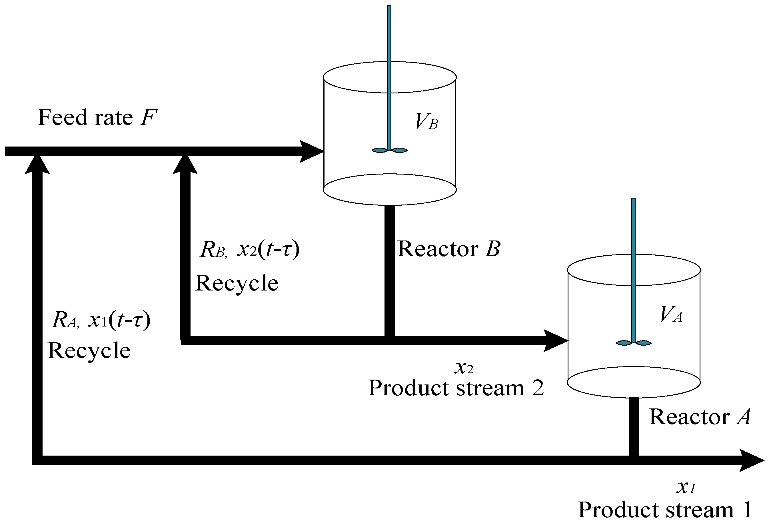
  43. Liu, L.; Yin, S.; Zhang, L.; Yin, X.; Yan, H. Improved results on asymptotic stabilization for stochastic nonlinear time-delay systems with application to a chemical reactor system. IEEE Trans. Syst. Man Cybern. Syst. 2016, 47, 195–204. [Google Scholar] [CrossRef]
  44. Hua, C.; Liu, P.X.; Guan, X. Backstepping control for nonlinear systems with time delays and applications to chemical reactor systems. IEEE Trans. Ind. Electron. 2009, 56, 3723–3732. [Google Scholar]
  45. Bolin, D.; Kovács, M.; Kumar, V.; Simas, A. Regularity and numerical approximation of fractional elliptic differential equations on compact metric graphs. Math. Comput. 2024, 93, 2439–2472. [Google Scholar] [CrossRef]
  46. Liu, Y.; Zhu, Q.; Fan, X. Event-triggered adaptive fuzzy control for stochastic nonlinear time-delay systems. Fuzzy Sets Syst. 2023, 452, 42–60. [Google Scholar] [CrossRef]
  47. Lin, W.; Qian, C. Adaptive control of nonlinearly parameterized systems: The smooth feedback case. IEEE Trans. Autom. Control. 2002, 47, 1249–1266. [Google Scholar] [CrossRef]
  48. Wang, H.; Chen, B.; Lin, C. Adaptive neural tracking control for a class of stochastic nonlinear systems. Int. J. Robust Nonlinear Control 2014, 24, 1262–1280. [Google Scholar] [CrossRef]
  49. Ai, Z.; Wang, H.; Niu, B.; Zhao, X. Fuzzy adaptive fixed-time output feedback tracking control for stochastic nonlinear systems with unmodeled dynamics. IEEE Trans. Fuzzy Syst. 2024, 32, 4074–4085. [Google Scholar] [CrossRef]
  50. Shao, S.; An, Z.; Chen, M.; Zhao, Q. Resilient neural control based on event-triggered extended state observers and the application in unmanned aerial vehicles. IEEE Trans. Intell. Veh. 2023, 9, 930–943. [Google Scholar] [CrossRef]
  51. Kanellakopoulos, I.; Kokotovic, P.V.; Morse, A.S. Systematic design of adaptive controllers for feedback linearizable systems. In Proceedings of the 1991 American Control Conference, Boston, MA, USA, 26–28 June 1991; pp. 649–654. [Google Scholar]
  52. Wang, H.; Liu, K.; Liu, X.; Chen, B.; Lin, C. Neural-based adaptive output-feedback control for a class of nonstrict-feedback stochastic nonlinear systems. IEEE Trans. Cybern. 2015, 45, 1977–1987. [Google Scholar] [CrossRef]
Figure 1. The backstepping technique.
Actuators 14 00019 g001
Figure 2. Two-stage chemical reactor with delayed recycle streams.
Actuators 14 00019 g002
Figure 3. The system tracking trajectories for Example 1.
Actuators 14 00019 g003
Figure 4. The trajectories of e under the proposed method and the method of [46] for Example 1.
Actuators 14 00019 g004
Figure 5. The trajectories of u and v for Example 1.
Actuators 14 00019 g005
Figure 6. The trajectories of x 2 and the constraint boundary functions for Example 1.
Actuators 14 00019 g006
Figure 7. The system tracking trajectories for Example 2.
Actuators 14 00019 g007
Figure 8. The trajectories of e under the proposed method and the method of [41] for Example 2.
Actuators 14 00019 g008
Figure 9. The trajectories of u and v for Example 2.
Actuators 14 00019 g009
Figure 10. The trajectories of x 2 and the constraint boundary functions for Example 2.
Actuators 14 00019 g010
Table 1. The practical significance and values of system parameters.
ParameterThe Practical SignificanceValue
R A Recirculation flow0.5 m3/s
R B Recirculation flow0.6 m3/s
G A Reactor residence time2 s
C A Reaction constant 0.5
C B Reaction constant 0.5
V A Reaction volume 0.4
V B Reaction volume1
FFeed rate0.5 m3/s
Table 2. Control performance index values of different methods.
Different MethodsTMTETMSSETECT
The proposed method0.20.0050.6
The method of [41]0.4420.051.525
Disclaimer/Publisher’s Note: The statements, opinions and data contained in all publications are solely those of the individual author(s) and contributor(s) and not of MDPI and/or the editor(s). MDPI and/or the editor(s) disclaim responsibility for any injury to people or property resulting from any ideas, methods, instructions or products referred to in the content.

