1. Introduction
Robots with flexible joints are becoming increasingly relevant. New types of robots are gaining importance on the market, such as collaborative robots (cobots), exoskeletons, and prostheses. They are meant to directly interact with humans. In this new generation of robots, the emphasis in their construction is not on precision (such as for rigid robot counterparts) but rather on weight reduction (collaborative robots) and/or soft interaction with humans (exoskeletons and prostheses). Thus, these new robots use more elastic mechanical transmissions.
Cobots typically have harmonic drive transmissions instead of classical gears [
1] due to their light weight, high reduction ratio, and relatively good back-driveability. Wearable robotics mostly use series elastic actuators (SEAs) [
2,
3] for transmission. SEAs are added to some cobots to increase the compliance of their harmonic drives [
4], such as those produced by the Rethink company.
Before the advent of flexible robots, most robots were rigid to achieve high precision. Controlling rigid manipulators is well covered and included in robotics textbooks [
5,
6,
7]. In these cases, the best performance is obtained using inverse dynamics control methods, also called computed torque. This involves compensating all nonlinear forces that act on the robot, such as gravity, inertia, and centrifugal and Coriolis forces.
When approaching the problem of controlling flexible robots, the first idea that comes to mind is adapting the well-known inverse dynamics method. However, in a rigid robot, the actuators are directly connected to the links, compensating for external forces. In a robot with flexible links, the motor acts on an elastic element, causing its torsion, which causes the link to move. Thus, the dynamic between the actuator and the link does not directly compensate for external forces.
Many applications involve a wide range of compliances in their joints. According to [
8], stiffnesses may vary from 5 to 10 kNm/rad down to 0.2 to 1 kNm/rad. This wide elasticity range complicates control considerably. In addition, stability analysis is much more difficult.
For example, oscillations may occur, possibly prohibiting many robotics tasks.
To achieve a task, the trajectory of the link () must be controlled, but it is only possible to act on the motor ().
Another complication in flexible robots vs. rigid ones is the higher order of the system. While the former is second-order, the latter is fourth [
9,
10]. Thus, it may be necessary to measure and include higher-order derivatives.
Several control strategies have been proposed to deal with this wide range of elasticity. The late 1980s and early 1990s were prolific regarding contributions in this field; researchers aimed to control motor position and velocity to achieve good trajectory tracking with links.
In [
11,
12], some less conventional control methods, like the
singular perturbation method (Spm) or
backstepping control design (Bcd), were proposed. Tomei [
13] introduced an extremely simple PD with the
simple gravity compensation (Sgc) method and demonstrated its stability criteria. The authors of [
14] improved the previous method, proposing
exact gravity cancellation (Egc) while introducing less restrictive criteria with better trajectory tracking. The authors of [
15,
16] introduced the
passivity-based approach (Pba) to determine the control action.
For each case, it is difficult to decide which method is appropriate and which constraints to use for its practical application, such as computational costs and expensive sensor requirements. Although some of these methods have been described in previous work [
11,
12,
17,
18], this study models and simulates a selection of methods to provide a clearer picture of the performance of each for different stiffness levels.
This study is dedicated to applying “classical” methods to control robots with flexible joints. A few recent strategies have not been included since they have several versions. Their analysis would be very extensive and has been left for future work. However, they are briefly mentioned below.
One approach is model predictive control (MPC) [
19,
20,
21]. This method includes constraints such as maximum motor torques and velocities in the controller design.
Another strategy is sliding mode control [
22,
23,
24]. It achieves good and robust trajectory tracking, but it may need a very fast sampling period.
Several authors have dedicated their research to robustly controlling robots with elastic joints [
25,
26,
27]. This is a wide area, and there are many very different contributions.
This paper is organized as follows: the
Section 2 presents the approach used to model the selected control algorithms. It then briefly describes the basis of each control algorithm and, finally, the simulation parameters. Then,
Section 3 presents the output of the simulations for different stiffness levels. Next,
Section 4 provides an interpretation of the simulation results, the requirements of each method for its practical implementation, and the pros and cons. Finally,
Section 5 discusses the advantages and disadvantages of each controller. At the end of the article,
Appendix A describes the first and second derivatives of the inertia, gravity, centrifugal, and Coriolis matrices.
2. Materials and Methods
2.1. Approaches for Modeling Robots with Flexible Joints
The dynamic model of the rigid robot is well known and can be found in textbooks [
5,
6,
7]. It can be represented by the following expression:
where
is the vector of the motor torque;
, and
are the vectors of the motor position, velocity, and acceleration, respectively;
is the inertia matrix of the robot;
is the matrix of the centrifugal and Coriolis forces; and
is the vector of gravity torques on the motors.
The following subsections describe the two possible ways to model the dynamics of robots with elastic joints: conventional modeling and the singularly perturbed model.
2.1.1. Conventional Elastic Modeling
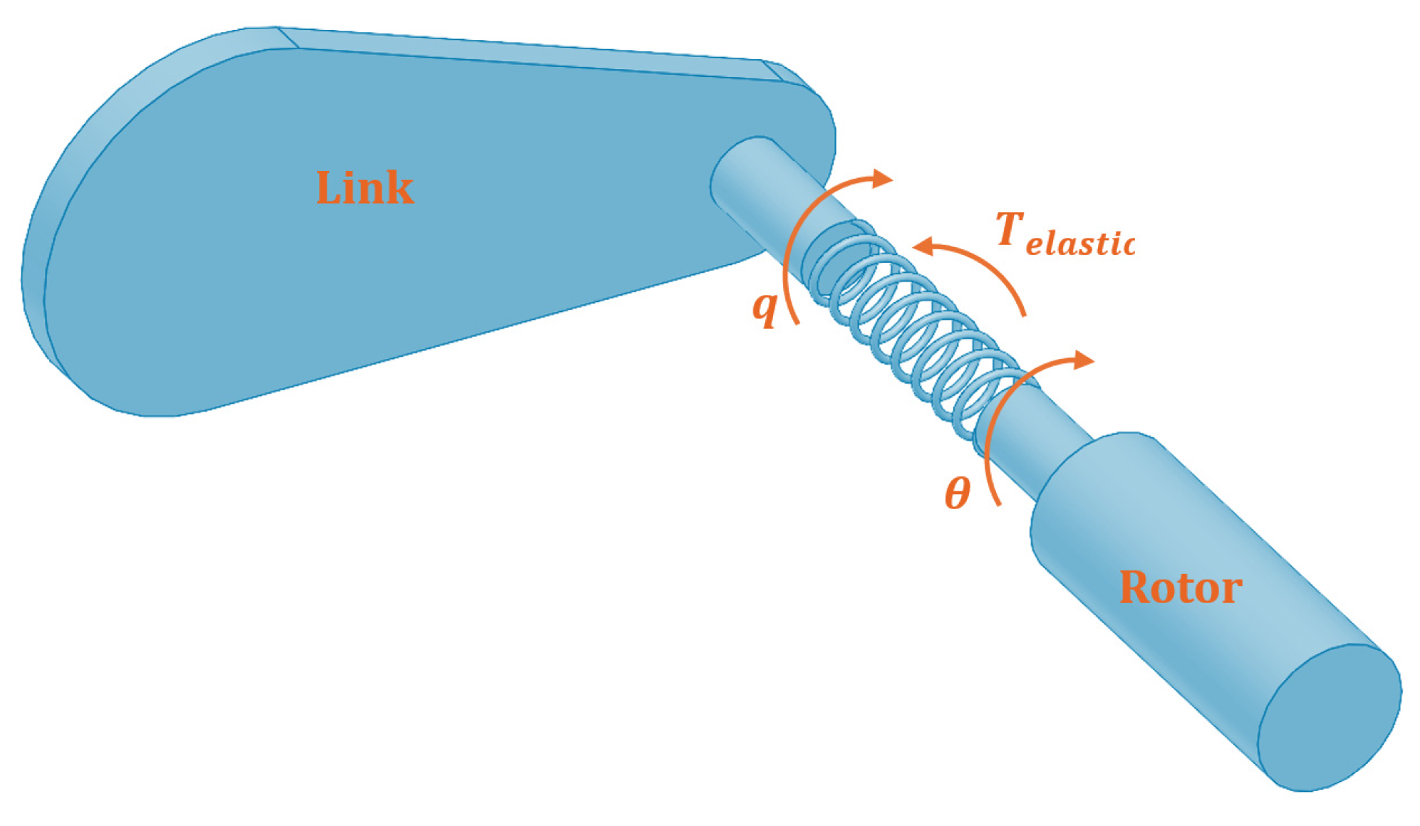
The main difference between modeling a rigid robot and a flexible robot is an elastic element between the motor rotor and the link (see
Figure 1).
The dynamics can be separated into two parts: the motor side and the link side. We can directly actuate the former, but we need to control the latter to achieve tasks, for example, as in [
17,
18]. This fact can be determined by assuming three conditions:
A1: Joint deflections are small, so flexibility effects are limited to the linear elasticity domain.
A2: Actuator rotors are modeled as uniform bodies with their centers of mass on the rotation axis.
A3: Each motor is located in the robot arm before the driven link. This can be generalized to the case of multiple motors simultaneously driving multiple distal links.
In this case, the complete model can be represented by the following expression:
where
is the vector of the motor torque;
,
, and
are the vectors of the link position, velocity, and acceleration, respectively;
,
, and
are the vectors of the rotor position, velocity, and acceleration, respectively;
is the inertia matrix of the robot;
the matrices of the centrifugal and Coriolis forces;
is the vector of gravity torque on the motors; and
is the elastic torque. The matrix,
S, represents the inertial coupling between the rotors and the links.
S is smaller than the other terms and is neglected by most authors, as are the
and
components, providing a reduced model:
This model is used for stability analysis in all of the studies mentioned in this article and, in general, by most authors. It will also be used in this study.
2.1.2. Singularly Perturbed Model
Another approach is using a singular perturbation model, that is, to refer to a situation in which a system exhibits two or more distinct time scales of motion. In these systems, one of the time scales is much slower than the others, separating the fast and slow dynamics. It was used in [
6,
11,
12,
13].
With a flexible joint, the elastic torque is much faster than the link. This separates the fast dynamics (elastic torque) from the slow dynamics (motion of the link). A singularly perturbated model can be obtained using a new coordinate space:
where
is the elastic torque.
If we assume that the matrix, , has large and similar elements, it is possible to extract a large common scale factor, , from : , .
Thus, Equation (8) can be rewritten as
Higher stiffness values mean lower values.
2.2. Control Strategies
This subsection briefly explains the control methods used in this study.
2.2.1. Singular Perturbation Method
The singular perturbation method [
28] control strategy is used for processes that have one part that is much faster than the other. This method treats the slow and the fast parts separately, making control much easier. Two control actions are generated: one for the slow part and another one for the fast one.
The output of the slow loop is used as the input for the fast loop. To obtain the final control action, slow and fast control actions are added.
For the slow part, the control action (torque) can be generated according to the laws of control for rigid robots, which have been known for decades, for example, the inverse dynamic method provided by Equation (4).
The fast control receives the slow control action as a reference value and must ensure that it will be tracked. According to [
18], a possible control law is
This is a PD control law for the elastic torque, and and are the proportional and derivative constants, respectively.
The final motor torque should be
Notably, the stability criteria for this control method are established according to the Tikhonov theorem [
28]. This states that if both the slow and fast loops are separately asymptotically stable and ϵ tends toward zero, their respective errors also tend toward zero. However, since
, it is greater than 0. Consequently, the convergence and stability cannot be determined analytically.
Since the convergence criteria assume that ε tends toward zero, the singular perturbation control will work better for robots with stiffer joints than robots with elastic ones.
This unclear stability criteria definition limits the singular perturbation method. It cannot be used for applications such as robust or adaptive control.
2.2.2. Backstepping Control Design
Backstepping control design [
29] is a control technique that stabilizes systems with nonlinear dynamics. It involves transforming the nonlinear dynamics into a series of intermediate systems with linear or linearizable dynamics and then applying a sequence of feedback controllers to each intermediate system, from top to bottom. The goal is to design a feedback control law that drives the system to its desired trajectory.
This system must be expressed so that each state variable derivative depends on this state, the next, and the previous ones. Only the last state derivative depends on the control action and all the previous states:
is a virtual input to guarantee the stability of . Then, is used as a virtual input to guarantee the stability of . This is repeated iteratively until the last state, which is stabilized by the control action, u.
This control method was first used to control elastic joints in [
11]. As will be demonstrated in simulations, this method works well. Nonetheless, it needs higher derivatives for the link position, and the system must be represented in a chained form, as in Equation (14).
2.2.3. Simple Gravity Compensation
Simple gravity compensation [
13] proposes a PD controller with gravity compensation. The control law is
where
is the reference position of the link.
Asymptotic stability is demonstrated for this case if , where is a number that fulfills the following condition for the given robot: .
This method is very simple. The reference position of the motors is necessary to compensate for the gravity torque of the links; it does not need the feedback of the link position. Only the motor position and velocity are used in the loop, helping to assure its stability.
2.2.4. Exact Gravity Cancellation
Exact gravity cancellation was proposed in [
14]. Its control action consists of two parts:
The first component dynamically compensates for gravity:
The second component is a PD-type law:
The global asymptotical stability can be shown via Lyapunov analysis. There are no constraints on the proportional constant.
This method is an improvement over the previous one.
2.2.5. Passivity-Based Approach
The passivity-based approach was proposed by the German Aerospace Center group and the Kuka company [
15,
16].
The final control law can be expressed as
is introduced for inertia shaping of the rotor since control is easier if the rotor and link inertias are similar orders of magnitude. The passivity of the system is thus demonstrated.
However, to obtain
, this method must compensate for the elastic torque and the feedback of the link velocity and acceleration to compute the inertia and centrifugal matrices. Regarding the elastic torque, the authors of [
16] proposed a lowpass filter with a cut-off frequency of 250 Hz.
Thus, it is necessary to compute up to the second derivatives of the inertia, centrifugal, and gravity matrices to obtain , which has a very high computational cost.
2.3. Modeling Robot Dynamics
The described control methods were modeled with MATLAB. The model assumes a two-degrees-of-freedom robot with revolute joints. The MATLAB files needed for the simulations are included in the
Supplementary Materials. There are five files, one for each controller. There is also a file called gentray5 that contains the fifth-order trajectory generator used by the other files.
The dynamics equations were obtained from [
17,
18]. For simplicity, the S inertia coupling matrix was set to 0 and the gear ratios to 1.
The links were modeled as uniform thin rods, with the following characteristics according to suggestions from experts in the field:
Their lengths are
Their masses are and .
The distances of the centers of gravity from the rotation axes are both .
Moments of inertia: and .
Gear ratios: .
Weight of the rotor of the second motor: .
Inertia carried by the second motor: .
Inertia carried by the first motor: .
The stiffnesses are set to , , and Nm/rad in different simulations.
Some intermediate variables were introduced:
For the dynamics expressed in Equation (2), the following matrix values were obtained:
2.4. Adjusting the Gains for the Controllers
All the controllers use some sort of feedback, typically proportional–derivative. Their performance will depend on their gains.
To control a single joint [
6], there are generally several (or infinite) combinations of proportional and derivative constants that work very well. They are computed based on the desired dynamics of the system, i.e., the natural frequency and damping ratio. To compute the proportional and derivative constants, it is necessary to know the inertia moment and the viscous friction coefficient of the system. Generally, better trajectory tracking is achieved with higher proportional and derivative gains. However, there is a point when increasing the gains practically does not improve the controller.
A multiple-degrees-of-freedom robot is much more complicated. The inertia carried by a motor is variable. Furthermore, centrifugal and Coriolis forces and gravity act on the links.
Most robot controllers (for rigid robots) compensate for the external forces and add a proportional–derivative controller for feedback [
5,
6,
7]. If all the dynamics (inertia, gravity, centrifugal forces) is compensated, the values of the proportional and derivative gains may be computed for the required natural frequency and damping ratio. However, when, for example, only gravity is compensated, the optimal values of the gains vary as the robot moves.
Usually, authors do not explain how these gains are obtained. One option is to adjust them through trial and error. Another is computing the value of the gains for each motor in real time, as in the case of a single joint, for the desired natural frequency and damping ratio of the system. However, this is time-consuming and not frequently used. Another method [
5] is gain scheduling. This involves reading the best gains for the actual robot configuration from a database in every sampling period.
In this study, the trial-and-error method was used. For every controller, many combinations were simulated. The simulations stopped when no more important improvements could be obtained.
3. Results
The simulations were conducted for a fifth-order polynomial trajectory generator. The first joint went from to and the second from to in five seconds.
The simulation was repeated for stiffnesses of
,
, and
Nm/rad for both joints. The first two values are typical for elastic mechanical transmissions like harmonic drives. A value of 200 is almost the most elastic found in the bibliographic research we conducted for this article [
30].
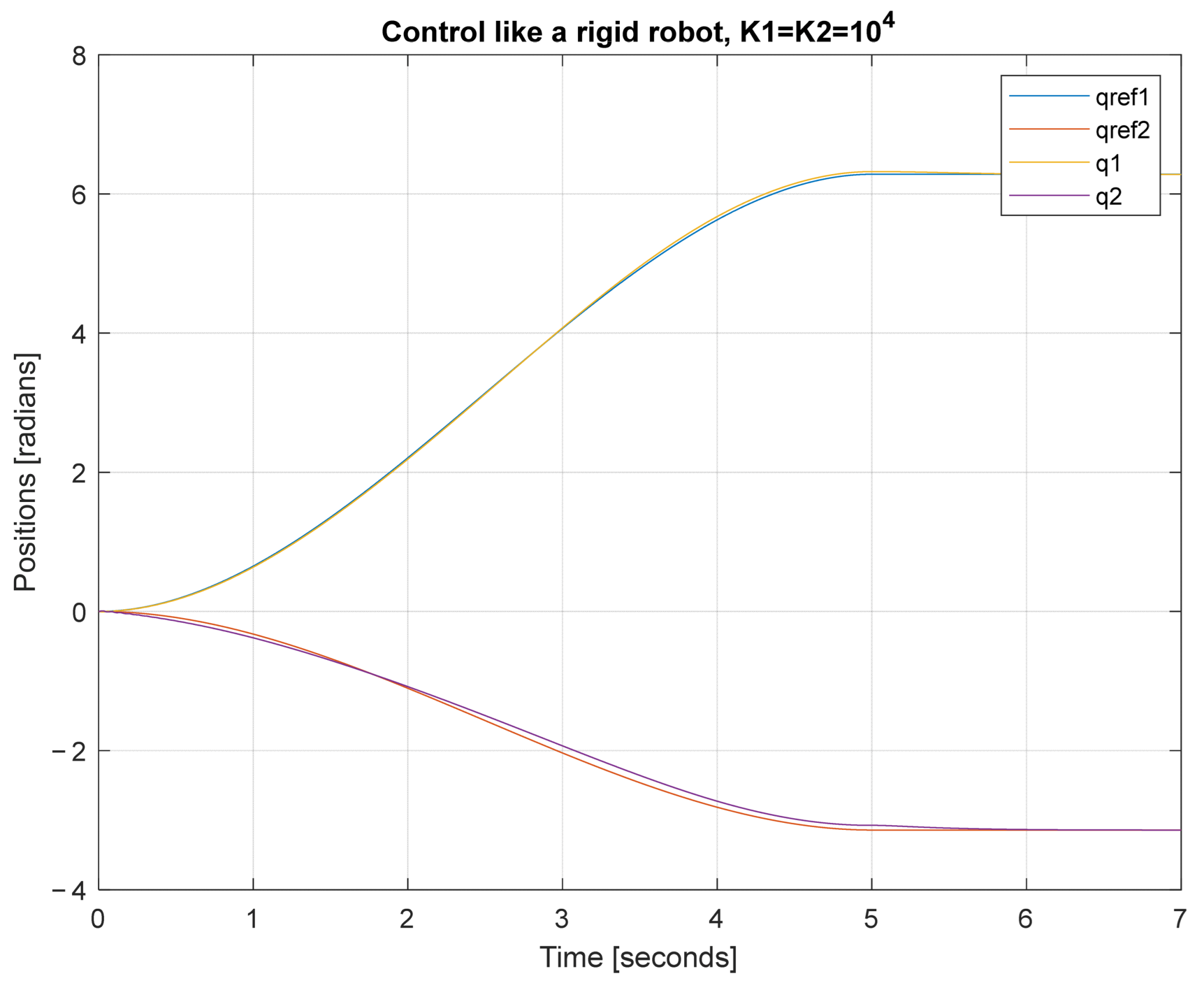
Before comparing the different controllers, simulations were conducted, controlling the robot as if it was rigid, i.e., directly compensating for the inertia, gravity, centrifugal, and Coriolis terms. For cases
and
, the system became unstable. For case
, it worked acceptably. Of course, this result also depends on the other dynamic parameters of the robot, such as its mass and moments of inertia.
Figure 2 shows the results of the simulation for
. The mean quadratic errors for both joints were 0.0006 and 0.0036.
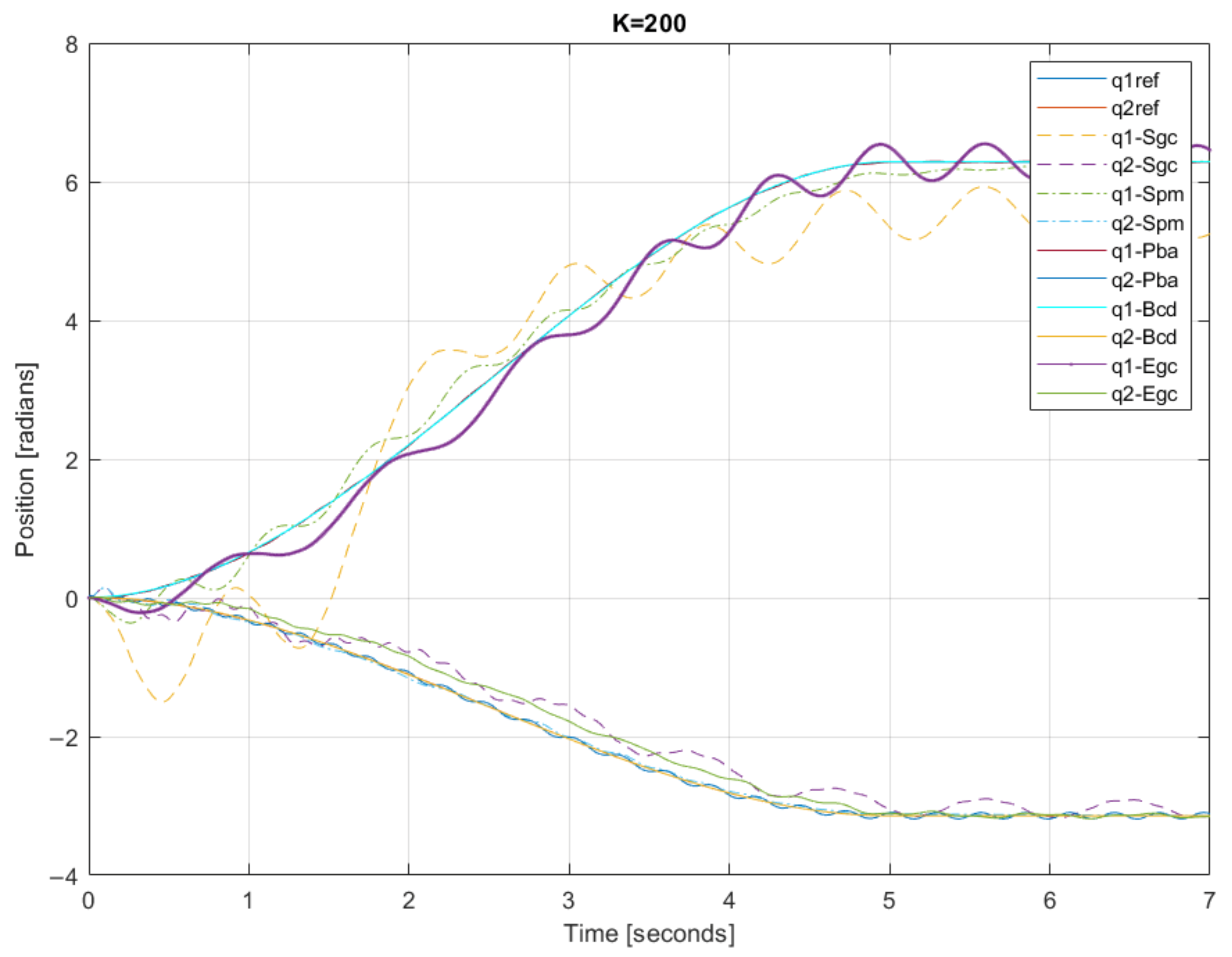
Then, the simulations were run for the different control strategies and stiffnesses. The simulation results for stiffness
are shown in
Figure 3, and the mean quadratic errors are shown in
Table 1.
The simulation results for stiffness
are shown in
Figure 4, and the mean quadratic errors are shown in
Table 2.
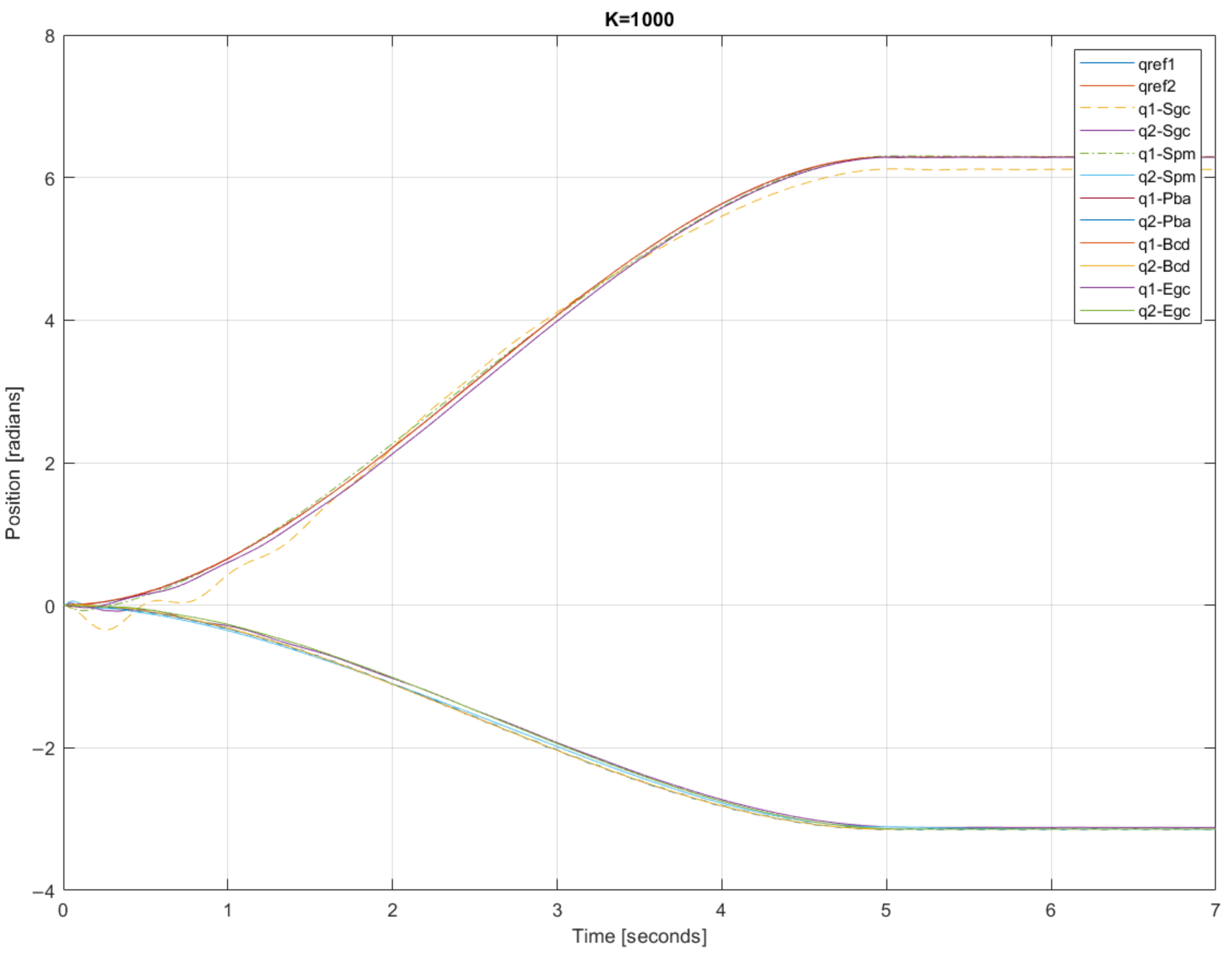
Finally, the simulation results for stiffness
are shown in
Figure 5, and the mean quadratic errors are shown in
Table 3.
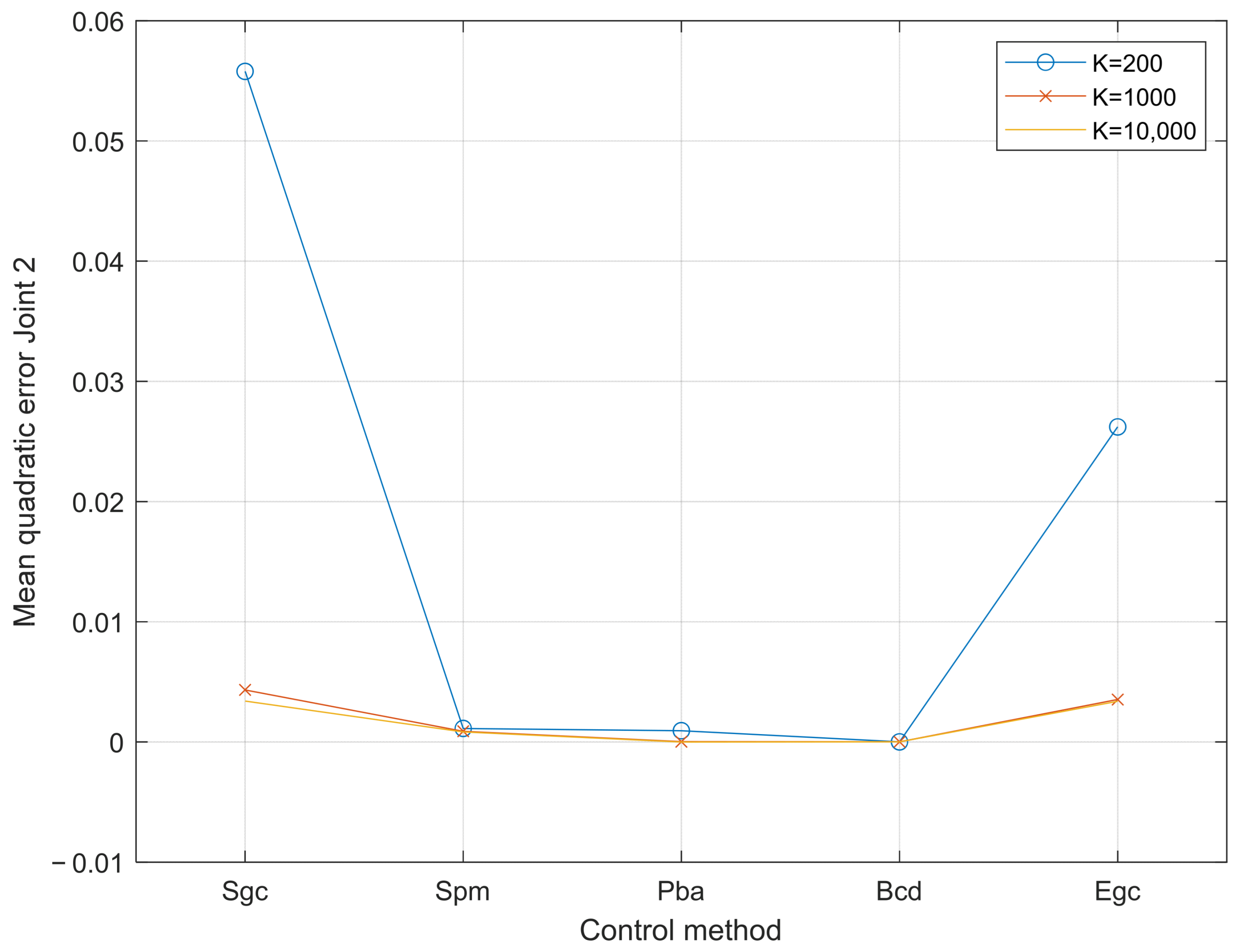
Figure 6 and
Figure 7 summarize the mean quadratic errors of the different methods for joint 1 and joint 2 for the three stiffness values.
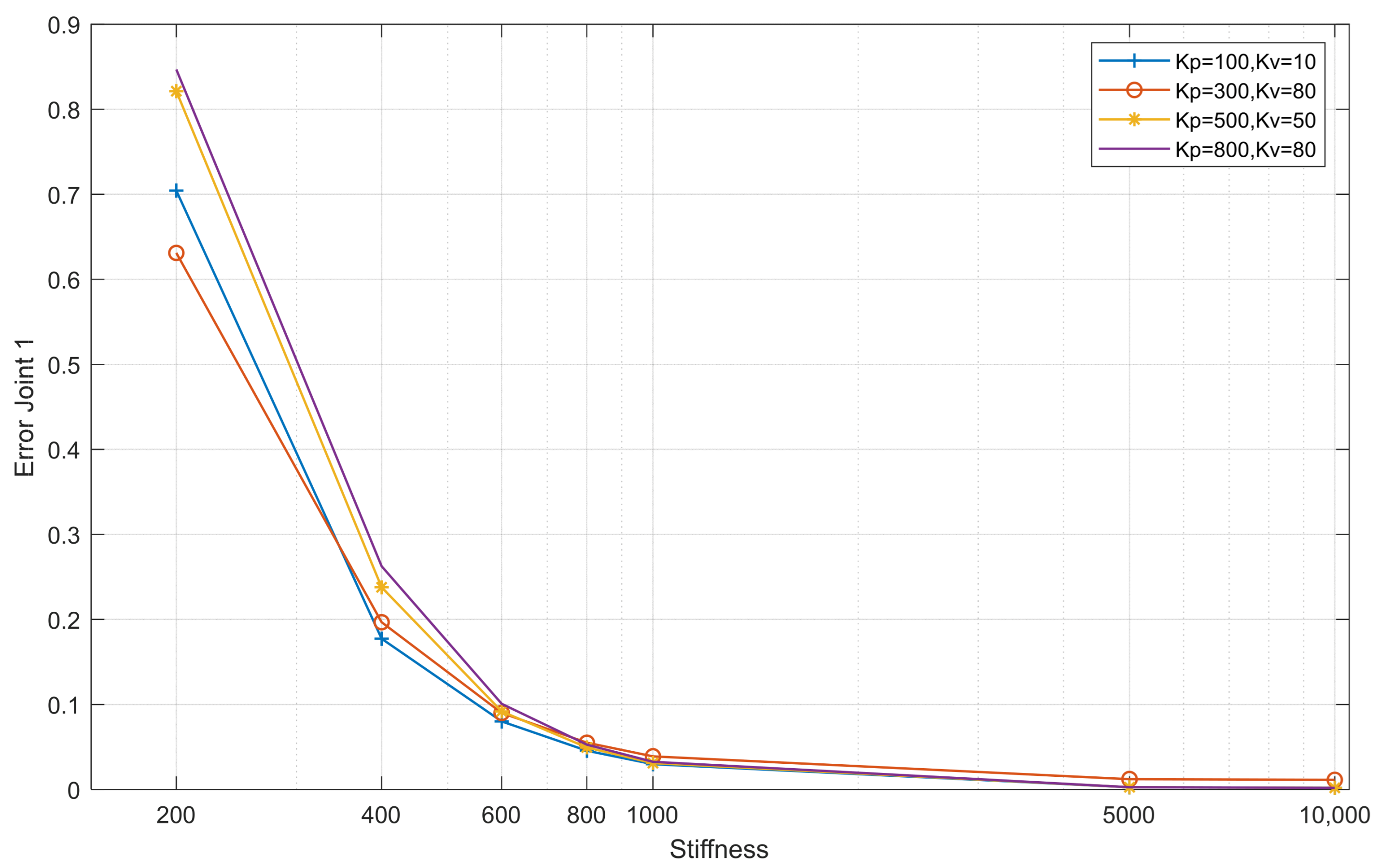
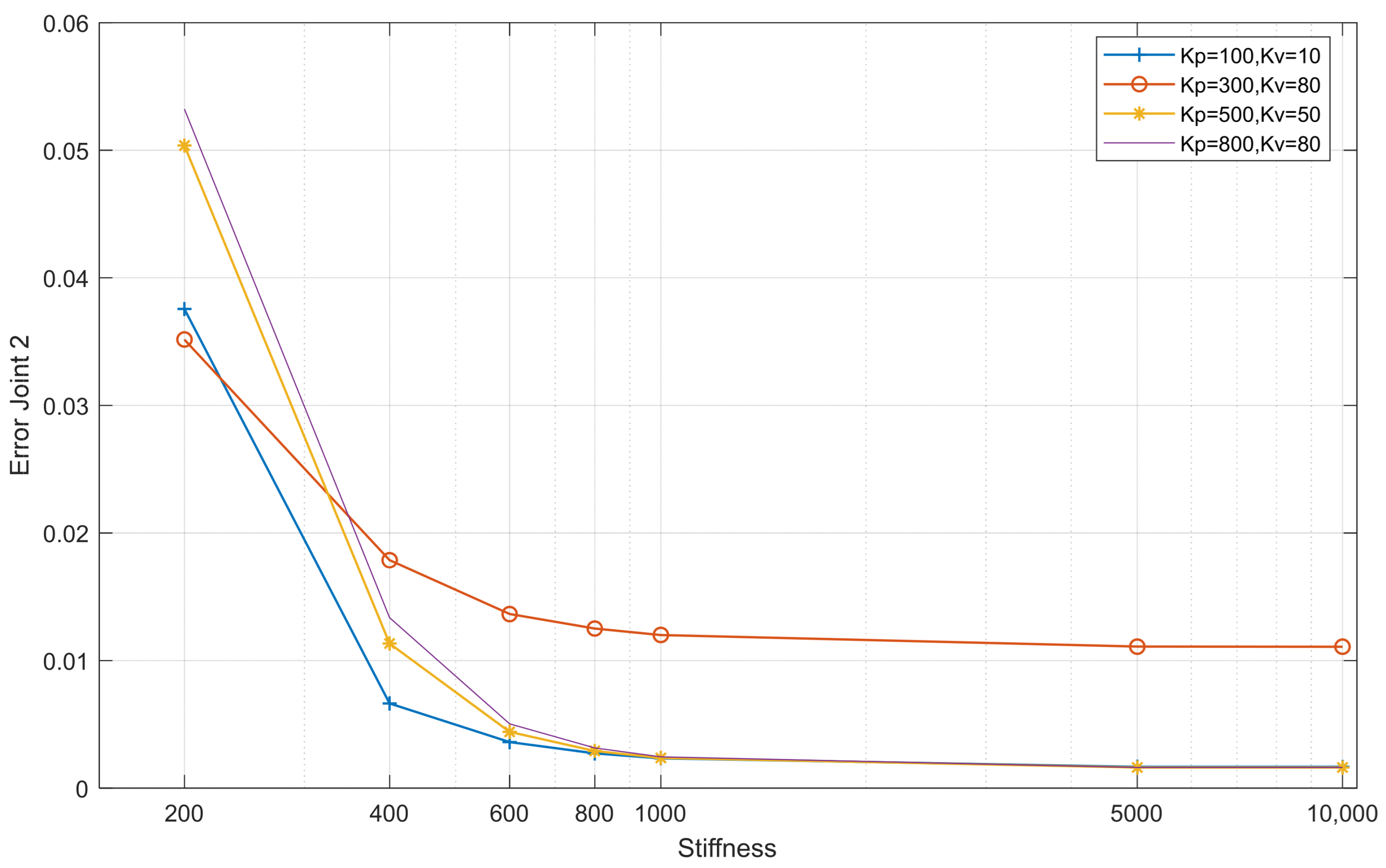
The results show that the simple gravity control method presents the highest position errors with many oscillations when the rigidity is 200. A specific analysis was carried out for this control method: First, the position error was evaluated for various levels of rigidity with values between 200 and 1000. In turn, the proportionality and derivative gains of this controller were modified to observe their influence.
Figure 8 and
Figure 9 show the position errors of each joint for different stiffness and controller gain levels.
In joint 1, the decreased error is more significant when stiffness increases. The controller gains may provide a minor error, but this is insignificant. For all controllers with low stiffnesses, the system oscillates. When the stiffness value reaches 600–800, the oscillations begin to disappear.
In joint 2, like joint 1, the error decreases as the stiffness increases; however, when low proportional gain and high derivative gain are used, a steady state error occurs with stiffnesses greater than 600.
4. Discussion
As expected, the simulations show that the errors are higher when the joint stiffness is lower. In addition, oscillations appear with low stiffness values for the Sgc, Spm, and Egc controllers.
Regarding mean quadratic errors, the Pba exhibits better results than the other controllers independently of the stiffness value.
The error in the first joint is one order of magnitude higher than that in the second joint, probably because the higher load carried by the first motor increases the nonlinearities. The error is much higher for K = 200 than for the other cases. The worst results are obtained with Sgc and then Egc. Spb is comparable to the Pba and Bcd for the second joint but not for the first one.
Although some controllers work very well in simulations, they need to measure or estimate certain magnitudes, such as the high derivatives of the position or torque. For example, position and velocity may be fed back using low-cost sensors and computer interfaces. However, many authors are reluctant to feed back the acceleration because of the significant effect of the noise. Few have used the first and second derivatives of acceleration (jerk and snap, respectively). Thus, the feasibility of these controllers in the real world is doubtful. The same problem occurs with torque feedback because torque measurements are noisy, and its derivative may be impossible to determine.
To summarize the requirements of each method,
Table 4 enumerates the necessary sensors and dynamic parameters.
More than one factor influences the complexity of the controller. One aspect is the necessary amount of computation. Another is the set of dynamic parameters that must be known. Some of these factors are not easy to identify, like moments of inertia. The dynamical parameters may vary from one robot to another even if they are the same model.
Another point to be considered is the necessary sampling period. A too-short sampling time may cause problems with real-time calculus and necessitate a more powerful computer. The necessary sampling time depends on the rate of change in the measured magnitude. Thus, typically, methods (e.g., Pba) that need to control the elastic torque need faster sampling than those that require only the positions and their derivatives.
From the cost perspective, position sensors are cheap, and they are necessary for all the control methods described in this article. However, adding torque sensors greatly increases the cost of the system.
The Spm works well for the stiffest case; however, it worsens as elasticity increases. For a stiffness of 200 Nm/rad, oscillations appear. This is logical since the initial supposition of this strategy is that the fast part is much faster than the slow one. On the other hand, the stability of this technique is determined by Tikhonov’s theorem [
28], which does not provide exact criteria for stability. This affects the robustness of the controller. In addition, the singular perturbation method requires a torque sensor and the first derivative of the elastic torque. Generally, this method is the third best regarding trajectory tracking.
The Bcd method has the second-best performance regarding trajectory tracking in simulations. However, it is hard to implement it in real applications since it requires feeding back higher-order derivatives.
The Sgc method is extremely simple and cheap (only sensors for the rotor position are required). It has the worst trajectory following, and its performance worsens as joint elasticity increases. For stiffnesses of 200 Nm/rad and 1000 Nm/rad, oscillations appear.
The Egc method is the second worst regarding trajectory tracking. It requires measuring the acceleration of the link to fully compensate the gravity. For a stiffness of 200 Nm/rad, oscillations appear.
The Pba has good performance regardless of joint stiffness. However, it requires an expensive torque sensor for each joint. The sampling period must be faster.
Since adjusting gains is an important part of controller design, a few words will be dedicated to this topic.
The Sgc and Egc methods have no feedback for the link position end velocity—just the motor side. Thus, the link works in an open loop. Varying the gains on the motor side cannot control the link side well for robots with relatively high elasticity.
The Spm has two sets of proportional–derivative gains: one for the fast part and another for the slow part. The fast part is very sensitive, and system stability can be easily lost with small variations in gains.
Regarding the Pba and Bcd methods, all relevant variables are fed back. These controllers are not approximative but exact methods. For these reasons, good trajectory tracking may be achieved with several gain combinations.
5. Conclusions
All the methods performed well for joints with small elasticity; however, oscillations appeared in Sgc for medium and high elasticity and Egc and the Spm for low stiffness.
Considering all the drawbacks and the advantages of the Spm, it is not the most advisable.
Egc is an improvement over simple gravity compensation. However, its small trajectory tracking upgrade does not justify the high derivative requirement or the increased computational cost.
The backstepping method has very good performance in simulations. However, its implementation in the real world is problematic.
In conclusion, the Sgc method is a fast and affordable solution if joint stiffness is relatively high. If good performance is necessary, the Pba is the best option.
