Article

Optimal Control-Based Algorithm Design and Application for Trajectory Tracking of a Mobile Robot with Four Independently Steered and Four Independently Actuated Wheels

by
Branimir Ćaran
1,
Vladimir Milić
1,*,
Marko Švaco
1 and
Bojan Jerbić
1,2
1
Faculty of Mechanical Engineering and Naval Architecture, University of Zagreb, HR-10000 Zagreb, Croatia
2
Croatian Academy of Sciences and Arts, HR-10000 Zagreb, Croatia
*
Author to whom correspondence should be addressed.
Actuators 2024, 13(8), 279; https://doi.org/10.3390/act13080279
Submission received: 30 May 2024 / Revised: 18 July 2024 / Accepted: 23 July 2024 / Published: 25 July 2024
(This article belongs to the Special Issue Actuators in 2024)

Abstract

:
This paper deals with the synthesis and implementation of a controller for asymptotic tracking of the desired trajectory of a mobile robot. The mobile robot used for the experimental validation has eight motors with an inner control loop. Four steering actuators are controlled using position controllers and four driving actuators are controlled using velocity controllers. A complex robot kinematic model is converted into a control-oriented linear time-varying system, which is then used to design a time-varying control law that minimizes the quadratic optimality criterion. In contrast to conventional methodologies for solving the corresponding Riccati differential equations, a computational approach that explicitly determines the time-varying controller matrix by employing recurrent matrix computations is proposed. Mobile robot control inputs (linear velocity, steering angles and steering velocities) are forwarded to the steering and driving actuators with properly tuned position and velocity controllers using an inverse kinematic model of the mobile robot. The obtained control law is evaluated on an experimental set-up of a real mobile robot system. The controller is implemented using the Robot Operating System.

1. Introduction

Following the significant advancements in both communication and information technologies, along with actuator and sensor technologies, a multitude of novel mobile robot systems have emerged, garnering substantial interest from both the scientific community and industrial and other applications. This interest has resulted in the publication of numerous review papers, representing a broad range of perspectives on the study and practical application of mobile robot technologies. Examples of this can be found in [1,2,3,4,5] among other places. It is now widely acknowledged that one of the key challenges in the development of efficient mobile robotic systems is the synthesis of algorithms for their trajectory tracking control [6].
Significant research and development has been undertaken in recent years with regard to robots with four wheels that have independent driving and steering. These developments have led to the application of various control strategies for this type of mobile robot system. In [7], the application of nonlinear model predictive control, wherein constraints are represented by the utilization of barrier functions for the guidance of a robot within a human-centric environment, has been proposed. In order to mitigate the latency in the steering angle response, the model predictive control algorithm with dynamic constraints for the tracking of high-speed trajectories was employed in [8]. A hybrid control approach integrating the sliding-mode control law, a near-time-optimal potential function and fuzzy-based adjustment rules were proposed in [9]. A direct yaw moment robust sliding-mode control strategy for a four-wheeled robot’s simultaneous trajectory tracking and disturbance rejection has been reported in [10]. Moreover, the control of four-wheeled mobile robots can be addressed in a comparable manner to that of autonomous vehicles. The principles and methods employed to solve control problems in these systems are analogous. For example, see [11,12,13,14,15,16] and related references.
This paper considers a mobile robotic structure with four independently steered and four independently actuated wheels (4ISW4IAW), part of an experimental set-up designed as a suitable laboratory model for the testing and verification of different control concepts and education. Details on this experimental set-up can be found in [17,18]. While this mobile robot was developed for climbing vertical walls, here we deal with the problem of following a reference trajectory on the ground.
In this paper, a trajectory tracking method for 4ISW4IAW mobile robot is presented. It is based on time-varying linear quadratic (TVLQ) control. Although the theoretical basis of the TVLQ approach is well established and can be considered a standard technique (see, for example, references [19,20] and the literature therein), the synthesis of controllers based on this approach remains a highly active area of research in a variety of applications, as evidenced, for example, by references [21,22,23,24]. Based on the available references, most studies in the area of TVLQ control have used one of two main approaches: the iterative approximate solution of the associated Riccati partial differential matrix equation or the transformation of the problem into a set of linear matrix inequalities (LMIs). It is well established that solving the Riccati equation requires the system to be fully controllable. However, our approach does not necessitate the resolution of the Riccati equation. The optimal control-based algorithm proposed in this paper is founded upon the direct numerical calculation of the time-varying elements of the control law matrix, without recourse to the LMI formalism or the approximation of the solution of the Riccati partial differential matrix equation.
In the approach proposed in this paper, we approximate the nonlinear three-input, two-chain, single-generator chained model of the 4ISW4IAW mobile robot with linear time-varying (LTV) differential error equations. The objective is to stabilize these equations in the vicinity of the desired trajectory. The control problem is defined in terms of determining a time-varying control law matrix that is calculated with respect to the minimization of the quadratic optimality criterion. A conjugate gradient method is employed to achieve a minimum value of the quadratic objective function. In order to determine the gradient, the chain rule for ordered derivatives is employed. The recursive matrix structure of the proposed algorithm is derived from the coupling of the control variables with the state variables, achieved through the use of the Euler method, which discretizes the kinematic equations of the robot.
The previously described method differs from other direct optimization methods in that the differential equations of the system are not treated as constraints that are included in the objective function by applying Lagrange multipliers or penalty functions. In contrast, our proposed approach explicitly leverages the connection between the control and state variables via discretized differential equations, thereby enabling the gradient of the objective function to be calculated with recursive relations. The fundamental concept behind this approach is presented in [25,26]. Here, this concept has been extended to include the synthesis of control laws for linear time-varying systems, which involved the derivation of an expression for the calculation of gradient values at each instant of the time interval.
Two main contributions of this work are as follows:
  • The Euler method for discretization, the conjugate gradient method and the line search method with Wolfe’s conditions for minimizing the objective function have been integrated into one numerically efficient algorithm for the direct calculation of the state controller of LTV systems. This algorithm explicitly obtains the desired time-variant control law.
  • The most effective version of the algorithm is subjected to both numerical simulations and experimental verification on a laboratory model of a 4ISW4IAW mobile robot system. Based on the authors’ current knowledge, the application and experimental verification of a time-varying controller designed in this way, which additionally includes the transformation into a three-input, two-chain, single-generator chained form, for a robot with four wheels that have independent drive and steer, has not been investigated yet.
The rest of the paper is organized as follows. In Section 2, a description of the experimental set-up of the mobile robot system under consideration is provided. Additionally, the kinematic model and its transformation into a three-input, two-chain, single-generator chained form are presented. The formulation of the trajectory tracking control problem in Section 3 involves approximating a nonlinear differential equation of the mobile robot in chained form with an LTV system. Subsequently, an algorithm for the synthesis of a time-varying state controller is derived. In Section 4, the simulation and experimental responses of the mobile robot system with the proposed control strategy are presented, along with a discussion related to the comparison with methods based on solving the Riccati equation or the LMI formalism. Section 5 concludes the paper.

2. System Description

2.1. Robot Description

The mobile robot used for experimental validation is designed to drive on vertical surfaces and perform nondestructive testing [18]. Figure 1 illustrates the mobile robot and its schematics. The robot is primarily constructed from acrylonitrile styrene acrylate (ASA) material using a 3D printing process, with some components made of carbon fiber [17]. The robot has dimensions of 380 × 300 mm, a total weight of 3.25 kg and a payload capacity of 1.5 kg. The mobile robot is equipped with eight direct current (DC) motors: four for steering and four for driving. Additionally, it features five brushless DC motors, four for thrust and one for the robot’s adhesion system. However, the thrust and adhesion motors are beyond the scope of this research, as the robot will only be operating on horizontal surfaces. The wheels are both driven and steered by Dynamixel XH430-W150 smart servo motors, with rotational positions monitored by AMS AS5601 magnetic rotary sensors.
The mobile robot is also equipped with a Raspberry Pi 4 Model B, running Linux Ubuntu and the Robot Operating System (ROS) as middleware. This set-up allows the execution of high-level control algorithms, logging of all data, and communication with the driving and steering motors. Communication with the Dynamixel motors is achieved using a ROBOTIS U2D2 USB to TTL converter, which relays steering and driving commands from ROS directly to the motors. As previously mentioned, the Dynamixel XH430-W150 smart servo motors have integrated proportional–integral–derivative (PID) control loops in various operation modes, including direct pulse-width modulation (PWM), current, velocity and position control modes. The robot’s driving motors are controlled using the velocity mode, while the steering motors are controlled using the position control mode. Figure 2 illustrates both the PI control loop for velocity and the PID control loop for position control modes.
The parameters for the DC motors were estimated in [27] using the Levenberg–Marquardt method. Both velocity and position controller gains were designed to ensure optimal performance in trajectory tracking for both velocity and position. Table 1 presents the calculated and estimated electro-mechanical parameters, where u a represents the armature voltage, R a and L a denote the armature resistance and inductance, K m and K e are the torque and back electromotive force constants, b d and b s are the driving and steering friction coefficients, and  J d and J s represent the inertia of the wheel and steering system (s marks steering and d marks driving system parameters).
Dynamixel DC motors are actuators which comprise a complete system. They feature an integrated PI control loop for the velocity and PID for position. Users are permitted to tune only the gains for those control loops. A PI controller is the preferred option for controlling DC motor velocity due to its simplicity and robustness, and the fact that it is able to meet the control requirements without the additional complications introduced by the derivative term. The inherent noise sensitivity of the derivative term, in conjunction with the existing mechanical filtering properties of the motor system, renders the use of a PID controller less desirable in many practical applications compared to the PI.
In Table 2, the controller gains of both the driving and steering systems are presented, where K v p and K v i are the proportional and integral gains of the PI velocity controller, respectively, and K p p , K p i and K p d are the proportional, integral and derivative gains of the PID position controller, and ω n represents the cut-off frequency of the 2nd order Bessel filter which cannot be changed.
All gains for control systems are chosen according to [27]. The proportional gain of the position control loop is adjusted in a way that prevented overshoot, ensuring a fast and smooth response. The PI control loop is tuned in a similar manner, allowing for a slight overshoot of 2%. During the tuning process, it is observed that, while using strong P gains for both the P position control loop and PI velocity control loop, there is a significant amount of chattering in the DC motor control loop, making it unsuitable for experimental validation. Later in the experimental section, the reference trajectory tracking of the driving velocity and steering angle will be shown using the control system parameters defined here.
Regarding the values presented in Table 2, in the context of position control, it is typically unnecessary to utilize integral and derivative gain (the values of K p i and K p d are zero), given that there are already two integrators following the output torque. The first of these is for velocity control, while the second is for position control. A proportional (P) controller offers a balance between simplicity, quick response and sufficient accuracy for numerous practical position control tasks, making it a preferred choice when these factors are prioritized.

2.2. Mathematical Model

The equations describing the kinematics of a mobile robot with four independently steered and four independently actuated wheels are given in [8,28], so they will not be detailed here. In this paper, we adopt assumptions from our recent work [29] to simplify the model from [8]. These assumptions enable a simpler derivation of the chain model and, consequently, a simpler derivation of the linear time-variant model of the robot. The main reason for the transformation into a chained form is the fact that direct Jacobian linearization of a nonlinear kinematic model would require predetermining the desired steering angle of all wheels, which would be quite complex in the case of some more demanding tracking trajectories.
We assume that the linear velocities of wheels are equal and the front and rear wheels are steered parallel to each other and at the same steering velocity. Hence, we obtain the following set of equations:
x ˙ = 1 2 cos ( δ 1 + θ ) + cos ( δ 2 + θ ) v 1 ,
y ˙ = 1 2 sin ( δ 1 + θ ) + sin ( δ 2 + θ ) v 1 ,
θ ˙ = x w 1 sin δ 1 2 x w 1 2 + 2 y w 1 2 + x w 2 sin δ 2 2 x w 2 2 + 2 y w 2 2 v 1 ,
δ 1 ˙ = ω 1 ,
δ 2 ˙ = ω 2 ,
where the reference point of the robot is represented by the coordinates x and y in the Cartesian frame, the orientation angle, denoted by θ , is expressed in relation to the positive x-axis, v 1 is the linear velocity, δ 1 , ω 1 , δ 2 and ω 2 are the steering angles and steering velocities of the front and rear wheels, respectively, and x w i and y w i , i = 1 , 2 , are the positions of the wheels predefined as follows: ( x w 1 , y w 1 ) = ( a , b ) and ( x w 2 , y w 2 ) = ( a , b ) where a and b are the lengths between the centroid of the robot and each wheel whose numerical values are a = b = 0.1125 m. Note that in (1)–(5) are five state variables—x, y, θ , δ 1 and δ 2 —and three input variables— v 1 , ω 1 and ω 2 .
System (1)–(5) can be transformed into the following three-input, two-chain, single-generator chained form
x ˙ 1 = u 1 ,
x ˙ 2 = u 2 ,
x ˙ 3 = x 2 u 1 ,
x ˙ 4 = u 3 ,
x ˙ 5 = x 4 u 1 .
by changing the coordinates as follows:
x 1 = x ,
x 2 = D 1 + D 2 c 1 + c 2 ,
x 3 = θ ,
x 4 = tan δ 1 + δ 2 2 + θ ,
x 5 = y ,
with the input transformation
u 1 = 1 2 c 1 + c 2 v 1 ,
u 2 = B 1 ω 1 + B 2 ω 2 ( c 1 + c 2 ) + ( D 1 + D 2 ) ( 2 ω 1 s 1 + 2 ω 2 s 2 ) 2 ( c 1 + c 2 ) + v 1 ( D 1 + D 2 ) 2 ( s 1 + s 2 ) 2 ( c 1 + c 2 ) 2 ,
u 3 = v 1 D 1 + D 2 + ω 1 + ω 2 K ,
where the following notation is introduced for the purpose of simplification:
c i = cos ( δ i + θ ) ,
s i = sin ( δ i + θ ) ,
B i = x w i cos ( δ i ) x w i 2 + y w i 2 ,
D i = x w i sin ( δ i ) x w i 2 + y w i 2 ,
K = 1 + cos ( δ 1 + δ 2 + 2 θ ) ,
for i = 1 , 2 .
In [29], the previous transformations are carried out in detail. To perform these transformations, it was necessary to apply the procedure from [30,31], where the conditions for the generalization of the chained form to systems with more than two inputs were derived.

3. Algorithm for the Synthesis of a Time-Varying State Controller

3.1. Control Problem Formulation

Based on [32], in this work, we formulate the trajectory tracking control problem utilizing the approach of approximating a nonlinear system of equations of a mobile robot in chained form (6)–(10) by an LTV system.
Let us assume that the desired trajectory in the Cartesian coordinate system is represented by x d ( t ) and y d ( t ) , while the desired orientation is θ d ( t ) = atan 2 y ˙ d ( t ) , x ˙ d ( t ) . Additionally, let us suppose that the desired trajectory is achievable. This implies the inputs
u d ( t ) = u d 1 ( t ) u d 2 ( t ) u d 3 ( t ) T ,
and the desired states
x d ( t ) = x d 1 ( t ) x d 2 ( t ) x d 3 ( t ) x d 4 ( t ) x d 5 ( t ) T ,
i.e., the reference robot can be calculated using (11)–(18). Furthermore, let us write the chained system (6)–(10) in standard vector notation:
x ˙ ( t ) = f ( x ( t ) , u ( t ) ) ,
where
x ( t ) = x 1 x 2 x 3 x 4 x 5 T , u ( t ) = u 1 u 2 u 3 T , f = u 1 u 2 x 2 u 1 u 3 x 4 u 1 T .
The Taylor expansion of system (26) around ( x d ( t ) , u d ( t ) ) , rejecting the terms of higher order, results in
x ˙ ( t ) = f ( x d ( t ) , u d ( t ) ) + f ( x d ( t ) , u d ( t ) ) x ( x ( t ) x d ( t ) ) + f ( x d ( t ) , u d ( t ) ) u ( u ( t ) u d ( t ) ) .
The state errors and input errors are defined as
x ˜ ( t ) = x ( t ) x d ( t ) , u ˜ ( t ) = u ( t ) u d ( t ) ,
respectively, and from (28) the LTV error equations are as follows:
x ˜ ˙ ( t ) = A ( t ) x ˜ ( t ) + B ( t ) u ˜ ( t ) ,
where
A ( t ) = f ( x d ( t ) , u d ( t ) ) x , B ( t ) = f ( x d ( t ) , u d ( t ) ) u .
Then, the control problem of tracking the desired trajectory is formulated as follows:
Problem 1.
Consider the LTV differential error equations (30) in which all state variables are available. The goal is to determine the control law of the form
u ˜ ( t ) = K ( t ) x ˜ ( t ) ,
where the matrix K ( t ) is determined according to the quadratic criterion of optimality, and thereby obtain the optimal control law of the form
u * = u d ( t ) K ( t ) x ˜ ( t ) ,
such that the system in chained form (6)–(10) is stabilized in the vicinity of the desired trajectory.
Problem 1 is known as local LQ trajectory stabilization [20], or the TVLQ control problem [19], and matrix K ( t ) can be calculated by solving the corresponding Riccati differential equation. It is important to note that solving the Riccati equation requires system (30) to be fully controllable. Nevertheless, the methodology presented in this paper avoids the necessity for solving the Riccati equation, instead relying on a direct numerical approach for minimizing the associated objective function.

3.2. Optimal Control-Based Algorithm Derivation

The optimal control-based algorithm for solving Problem 1, as presented in this paper, employs a representation of control vector components as linear functions of state variables with time-varying parameters. The aforementioned parameters are, in fact, elements of the matrix K ( t ) , which must be determined.
In order to write the control law (32) in a parametrized form, the vectorization operator (the operator vec ( · ) is an operator that stacks the columns of a matrix one underneath the other) can be applied:
vec u ˜ ( t ) = vec K ( t ) x ˜ ( t ) = x ˜ T ( t ) I vec K ( t ) .
In this context, the symbol ⊗ denotes the Kronecker product, while the identity matrix I has the same number of rows as the matrix K ( t ) . In order to facilitate further analysis, the control law is introduced in the following notation.
u ˜ ( t ) = X ˜ ( t ) k ( t ) ,
where X ˜ ( t ) = x ˜ T ( t ) I and k ( t ) = vec K ( t ) .
The problem of finding k ( t ) in a control law (35) is based on the minimization of the objective function
J = 0 t f x ˜ T ( t ) Q x ˜ ( t ) + u ˜ T ( t ) R u ˜ ( t ) d t ,
for all t f 0 with Q = Q T 0 , R = R T > 0 subject to the error equations (30).
Remark 1.
Note that the objective function (36) implicitly depends on elements of k ( t ) from (35), so the matrix K ( t ) in (32) can be determined after appropriate reshaping of the vector k ( t ) .
Our approach can be classified as a direct optimization method, whereby a continuous-time system is transformed into a discrete-time system. It can therefore be assumed that the time interval 0 , t f is divided into N 1 sub-intervals of equal length. The resulting time grid is then composed of points t i = i τ , where i = 0 , 1 , 2 , , N 1 and τ is defined as the time step length, with a value of t f / N . Subsequently, the Euler approximation of the continuous-time state Equation (30) is
x ˜ ( i + 1 ) = x ˜ ( i ) + τ A ( i ) x ˜ ( i ) + B ( i ) u ˜ ( i ) , x ˜ ( 0 ) = x ˜ 0 .
The discretized control law (35) can be expressed as
u ˜ ( i ) = X ˜ ( i ) k ( i ) .
The discrete-time form of the objective function (36) with (38) results in
J = τ i = 0 N 1 x ˜ T ( i ) Q x ˜ ( i ) + k T ( i ) X ˜ T ( i ) R X ˜ ( i ) k ( i ) .
Considering everything mentioned above, the optimization problem can be summed up as follows:
min k ( i ) τ i = 0 N 1 x ˜ T ( i ) Q x ˜ ( i ) + k T ( i ) X ˜ T ( i ) R X ˜ ( i ) k ( i ) , subject to :
x ˜ ( i + 1 ) = x ˜ ( i ) + τ A ( i ) x ˜ ( i ) + B ( i ) X ˜ ( i ) k ( i ) , x ˜ ( 0 ) = x ˜ 0 .
The main concept of the proposed approach to solving the optimization problem (40) and (41) is based on the integration of a conjugate gradient method and line search method with Wolf conditions into one algorithm which uses recursive matrix relations to compute the first-order derivatives and provide a direct numerical calculation of the time-varying elements of vector k . The minimization in (40) is performed by a conjugate gradient descent algorithm in the following form
k ( l + 1 ) ( j ) = k ( l ) ( j ) + η s ( l ) ( j ) ,
s ( l + 1 ) ( j ) = J k ( j ) ( l + 1 ) + β s ( l ) ( j ) ,
for j = 0 , 1 , 2 , , N 1 and l = 0 , 1 , 2 , , M . N is the number of time instants, M is the number of gradient algorithm iterations and  s is the search direction vector. Here we note that all vectors in (42) and (43) are column vectors including the gradient of the objective function. This should be kept in mind in later expressions so that the dimensions of matrices and vectors are not misunderstood.
The standard method for computing β is
β = μ J k T ( j ) ( l + 1 ) J k ( j ) ( l + 1 ) + [ 1 μ ] J k T ( j ) ( l + 1 ) J k ( j ) ( l + 1 ) J k ( j ) ( l ) ν J k T ( j ) ( l ) J k ( j ) ( l ) + [ 1 ν ] s T ( l ) J k ( j ) ( l + 1 ) J k ( j ) ( l ) .
It should be noted that in (44) there are four distinct possible combinations for the parameters μ and ν that can be utilized in accordance with references [33,34,35,36].
In order to find the convergence step η > 0 , we employ a line search strategy with the Wolfe conditions. The method of line search with Wolf’s conditions is considered quite standard and well-known, and there is no need to present it in detail here. Further details about Wolfe conditions and the line search technique are available in [37].
In the l-th iteration of (42) and (43) the gradient of the objective function with respect to k is given by
J k ( j ) = τ i = 0 N 1 x ˜ T ( i ) Q x ˜ ( i ) + k T ( i ) X ˜ T ( i ) R X ˜ ( i ) k ( i ) k ( j ) = = τ x ˜ T ( j ) Q x ˜ ( j ) + k T ( j ) X ˜ T ( j ) R X ˜ ( j ) k ( j ) k ( j ) + i = j + 1 N 1 x ˜ T ( i ) Q x ˜ ( i ) + k T ( i ) X ˜ T ( i ) R X ˜ ( i ) k ( i ) k ( j ) ,
for j = 0 , 1 , 2 , , N 1 , where the terms with i < j are equal to zero.
Obviously, in the previous expression, the first term in parentheses is
x ˜ T ( j ) Q x ˜ ( j ) + k T ( j ) X ˜ T ( j ) R X ˜ ( j ) k ( j ) k ( j ) = 2 X ˜ T ( j ) R X ˜ ( j ) k ( j ) .
Since the second term in the parentheses in (45) depends on k ( j ) implicitly through x ˜ ( i ) for i > j , in what follows, we will derive recursive relations for its computation. Using the basic chain rule arithmetic, the term in the sum of (45) is
x ˜ T ( i ) Q x ˜ ( i ) + k T ( i ) X ˜ T ( i ) R X ˜ ( i ) k ( i ) k ( j ) = = x ˜ ( i ) k ( j ) x ˜ T ( i ) Q x ˜ ( i ) + k T ( i ) X ˜ T ( i ) R X ˜ ( i ) k ( i ) x ˜ ( i ) = = 2 x ˜ ( i ) k ( j ) Q x ˜ ( i ) + x ˜ ( i ) k ( j ) k T ( i ) X ˜ T ( i ) R X ˜ ( i ) k ( i ) x ˜ ( i ) .
Note that x ˜ R 5 , k R 15 and x ˜ ( i ) k ( j ) R 15 × 5 ; thus, the above expression is dimensionally well defined.
From (41) it follows that
x ˜ ( j + 1 ) k ( j ) = τ X ˜ T ( j ) B T ( j ) , x ˜ ( i ) k ( j ) = x ˜ ( i 1 ) k ( j ) I + τ A ( i 1 ) ,
for i = j + 2 , , N 1 .
Next, let us denote the sum from Equation (45) by
Σ j = i = j + 1 N 1 x ˜ T ( i ) Q x ˜ ( i ) + k T ( i ) X ˜ T ( i ) R X ˜ ( i ) k ( i ) k ( j ) .
Based on (47) for j = N 2 , i = N 1 , it follows
Σ N 2 = 2 x ˜ ( N 1 ) k ( N 2 ) Q x ˜ ( N 1 ) + x ˜ ( N 1 ) k ( N 2 ) k T ( N 1 ) X ˜ T ( N 1 ) R X ˜ ( N 1 ) k ( N 1 ) x ˜ ( N 1 ) .
Substituting (48) in (50), we obtain
Σ N 2 = 2 τ X ˜ T ( N 2 ) B T ( N 2 ) Q x ˜ ( N 1 ) + τ X ˜ T ( N 2 ) B T ( N 2 ) k T ( N 1 ) X ˜ T ( N 1 ) R X ˜ ( N 1 ) k ( N 1 ) x ˜ ( N 1 ) .
Furthermore, for  j = N 3 , i = N 1 , N 2 from (47), it follows
Σ N 3 = 2 x ˜ ( N 2 ) k ( N 3 ) Q x ˜ ( N 2 ) + x ˜ ( N 2 ) k ( N 3 ) k T ( N 2 ) X ˜ T ( N 2 ) R X ˜ ( N 2 ) k ( N 2 ) x ˜ ( N 2 ) + 2 x ˜ ( N 1 ) k ( N 3 ) Q x ˜ ( N 1 ) + x ˜ ( N 1 ) k ( N 3 ) k T ( N 1 ) X ˜ T ( N 1 ) R X ˜ ( N 1 ) k ( N 1 ) x ˜ ( N 1 ) .
Substituting (48) in (52), we obtain
Σ N 3 = 2 τ X ˜ T ( N 3 ) B T ( N 3 ) Q x ˜ ( N 2 ) + τ X ˜ T ( N 3 ) B T ( N 3 ) k T ( N 2 ) X ˜ T ( N 2 ) R X ˜ ( N 2 ) k ( N 2 ) x ˜ ( N 2 ) + 2 τ X ˜ T ( N 3 ) B T ( N 3 ) I + τ A ( N 2 ) Q x ˜ ( N 1 ) + τ X ˜ T ( N 3 ) B T ( N 3 ) I + τ A ( N 2 ) · k T ( N 1 ) X ˜ T ( N 1 ) R X ˜ ( N 1 ) k ( N 1 ) x ˜ ( N 1 ) , Σ N 3 = τ X ˜ T ( N 3 ) B T ( N 3 ) · { 2 Q x ˜ ( N 2 ) + k T ( N 2 ) X ˜ T ( N 2 ) R X ˜ ( N 2 ) k ( N 2 ) x ˜ ( N 2 ) + I + τ A ( N 2 ) · 2 Q x ˜ ( N 1 ) + k T ( N 1 ) X ˜ T ( N 1 ) R X ˜ ( N 1 ) k ( N 1 ) x ˜ ( N 1 ) } .
The preceding procedure can be carried out in the following manner:
Σ N 4 = τ X ˜ T ( N 4 ) B T ( N 4 ) · { 2 Q x ˜ ( N 3 ) + k T ( N 3 ) X ˜ T ( N 3 ) R X ˜ ( N 3 ) k ( N 3 ) x ˜ ( N 3 ) + I + τ A ( N 3 ) · 2 Q x ˜ ( N 2 ) + k T ( N 2 ) X ˜ T ( N 2 ) R X ˜ ( N 2 ) k ( N 2 ) x ˜ ( N 2 ) + I + τ A ( N 2 ) · 2 Q x ˜ ( N 1 ) + k T ( N 1 ) X ˜ T ( N 1 ) R X ˜ ( N 1 ) k ( N 1 ) x ˜ ( N 1 ) } .
Finally, based on the previous derivations from (45) to (54), the recursive relations for calculating the gradient in (43) are
κ N 1 = 0 ,
κ j = 2 Q x ˜ ( j + 1 ) + k T ( j + 1 ) X ˜ T ( j + 1 ) R X ˜ ( j + 1 ) k ( j + 1 ) x ˜ ( j + 1 )
+ I + τ A ( N 2 ) κ j + 1 ,
Σ j = τ X ˜ T ( j ) B T ( j ) κ j ,
J k ( j ) = τ 2 X ˜ T ( j ) R X ˜ ( j ) k ( j ) + Σ j ,
for j = N 2 , N 3 , , 0 .
The algorithm described above is summarized in the following steps:
  • For the Euler approximation (37); set the initial state vector x 0 ; set final time t f ; set number of time intervals N; calculate time step length τ .
  • Choose the weight matrices Q , R and an arbitrary initial values of k for the objective function (40).
  • For the conjugate gradient descent algorithm (42) and (43), set number of iterations M; choose initial convergence rates β and η .
  • For everything previously initialized, first calculate the state vector using the Euler method (41) and then calculate the initial search direction vector according to (59) as s = J k .
  • Calculate the new k using (42).
  • Calculate the gradient J k using recursive matrix expressions from (55) to (59).
  • Calculate the new convergence rate β from (44) and new search direction vector s using (43). In order to determine new step-size η in (42), employ the line search strategy satisfying the Wolfe conditions as outlined in reference [37].
  • Calculate the state vector using the Euler method (41).
  • Shift l = l + 1 in (42) and (43) and go back to step 5.

4. Simulation and Experimental Validation

4.1. Simulation Results

This subsection presents the results of a simulation conducted to assess the effectiveness of a controller synthesis procedure, previously described in detail in preceding sections of this work.
The matrices A ( t ) and B ( t ) from (31) are defined as follows:
A ( t ) = 0 0 0 0 0 0 0 0 0 0 0 u d 1 ( t ) 0 0 0 0 0 0 0 0 0 0 0 u d 1 ( t ) 0 , B ( t ) = 1 0 0 0 1 0 x d 2 ( t ) 0 0 0 0 1 x d 4 ( t ) 0 0 ,
and thus the LTV system (30) is determined, for which the synthesis of control law (32) is performed. The algorithmic procedure, described in Section 3.2 for calculating the time-varying elements of the vector k ( t ) at each discrete point of the time interval, by solving the optimization problem (40) and (41), which is then reshaped into the controller matrix K ( t ) , has been implemented in the C programming language.
The tracking of reference trajectories is considered in three cases: straight line, circle and curvilinear. In all three cases, the time step length for discretization by the Euler method is set to τ = 0.016 s. This is consistent with the sampling frequency of the experimental set-up, which is 62.5 Hz. Moreover, in order to calculate the convergence rate β from Equation (44), the values of μ and ν are set to 1 and 0, respectively. This involved the application of the Dai-Yuan method [36]. All calculations are performed on a standard portable computer.
Figure 3 shows a block diagram of the entire control strategy for trajectory tracking.

4.1.1. Straight Line Trajectory Tracking

The desired straight line trajectory is defined as follows:
x d ( t ) = 1 20 t , y d ( t ) = 1 20 t , θ d ( t ) = atan 2 y ˙ d ( t ) , x ˙ d ( t ) = π 4 .
In order to obtain the reference of the robot, (61) together with (11)–(15) is included in (6)–(10), from which the desired robot states are calculated as follows:
x d 1 = 1 20 t , x d 2 = 0 , x d 3 = π 4 , x d 4 = 1 , x d 5 = 1 20 t ,
and the desired inputs are calculated as follows:
u d 1 = 1 20 , u d 2 = 0 , u d 3 = 0 .
The simulation results of tracking a straight line are shown in Figure 4 and Figure 5. The initial time is t 0 = 0 s, the final time is t f = 40 s and the number of optimization time intervals is N = 2500 . The initial positions and orientation angle of the robot are set to x ( t 0 ) y ( t 0 ) θ ( t 0 ) = 0 0 0 . The weight matrices Q and R of the objective function are chosen as Q = diag ( 10 3 , 1 , 10 2 , 1 , 10 3 ) and R = diag ( 10 4 , 10 2 , 10 2 ) .
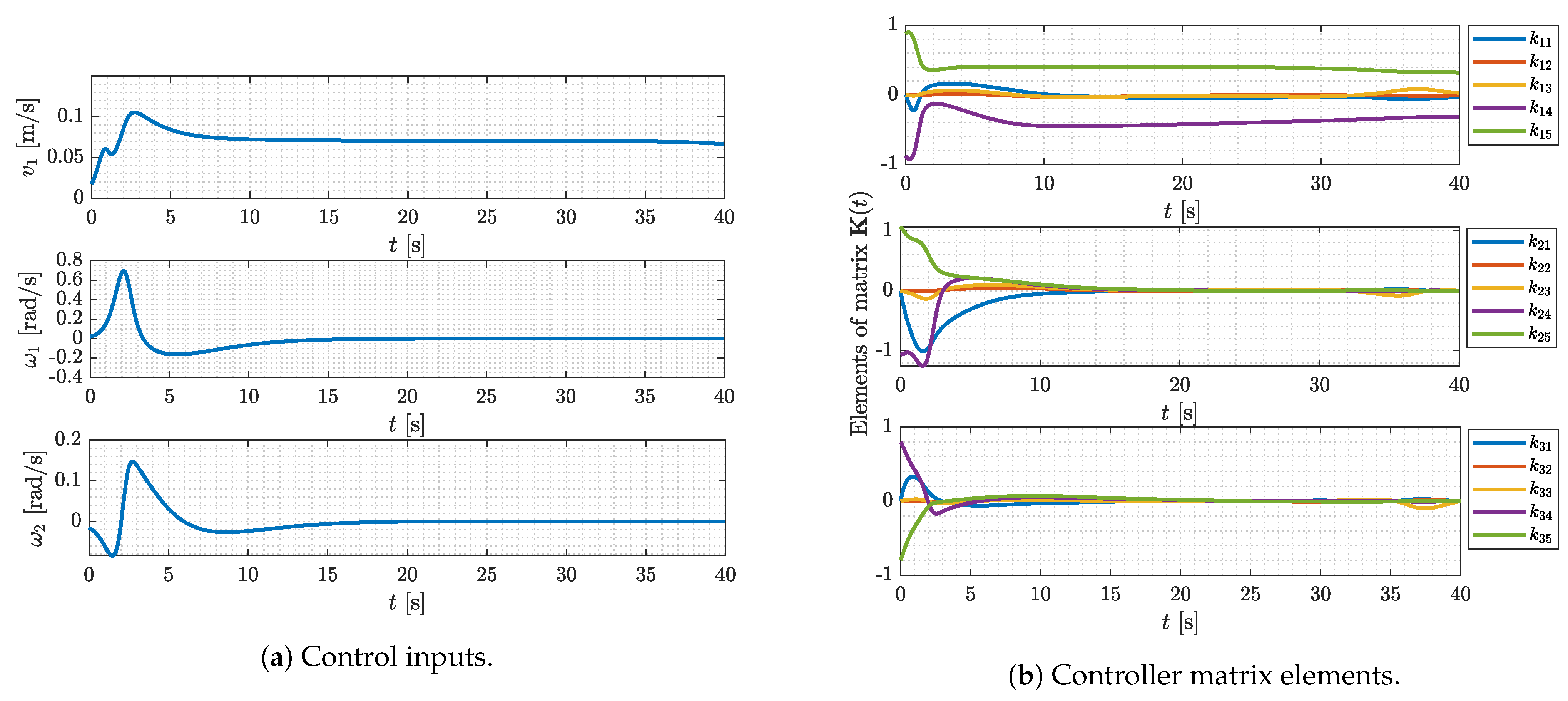
In Figure 4a, it can be seen that after the transition from the initial conditions the robot follows the desired trajectory very well. Time responses of positions x and y, orientation angle θ , and steering angles δ 1 and δ 2 are shown in Figure 4b and Figure 4c, respectively. Furthermore, the time responses of control inputs, i.e., linear velocity v 1 and steering velocities ω 1 and ω 2 , are shown in Figure 5a. From their responses and maximum values, it can be seen that these velocities are achievable on the actuators of the experimental set-up of the 4ISW4IAW mobile robot. On the experimental mobile robot, due to certain mechanical limitations, but also due to applications for other purposes, the maximum value of v 1 is set to 0.13  m/s. The time dependencies of the elements of the state controller matrix calculated by the proposed algorithm are shown in Figure 5b.

4.1.2. Circular Trajectory Tracking

The desired circular trajectory is defined as follows:
x d ( t ) = sin ω t , y d ( t ) = 1 cos ω t , θ d ( t ) = atan 2 y ˙ d ( t ) , x ˙ d ( t ) ,
where ω = 2 π t f and t f is the final time. In order to obtain the reference of the robot, (64) together with (11)–(15) is included in (6)–(10), from which the desired robot states are calculated as follows:
x d 1 = sin ω t , x d 2 = 1 cos ω t , x d 3 = arctan tan ω t , x d 4 = tan ω t , x d 5 = 1 cos ω t ,
and the desired inputs are calculated as follows:
u d 1 = ω cos ω t , u d 2 = ω sin ω t sin ω t 2 1 , u d 3 = ω sin ω t 2 1 .
Remark 2.
In order to eliminate the discontinuities caused by the tan (·), arctan ( · ) and atan2 ( · ) functions, it is necessary to add multiples of ± 2 π when the phase difference between consecutive angles of y ˙ d ( t ) , x ˙ d ( t ) exceeds π radians.
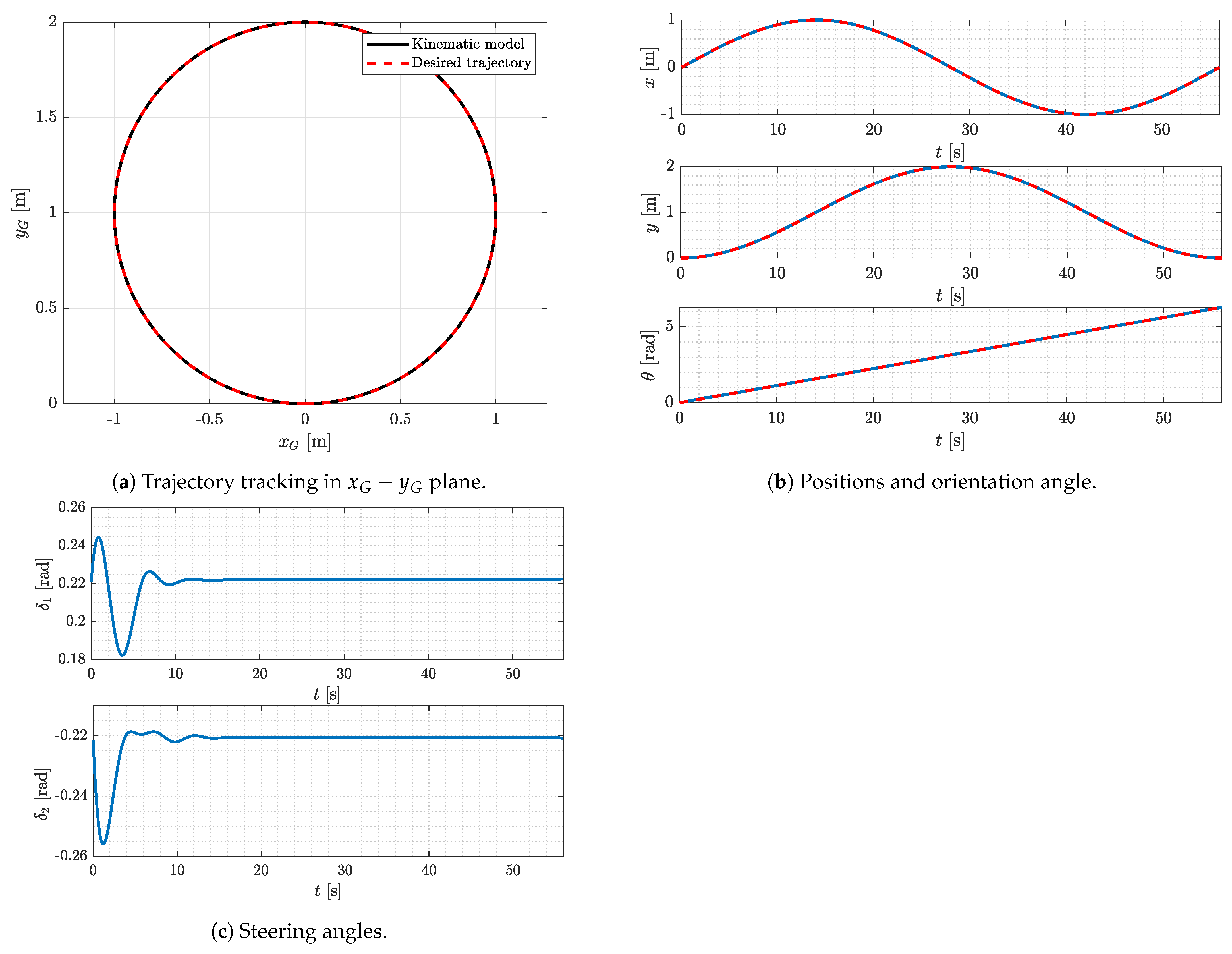
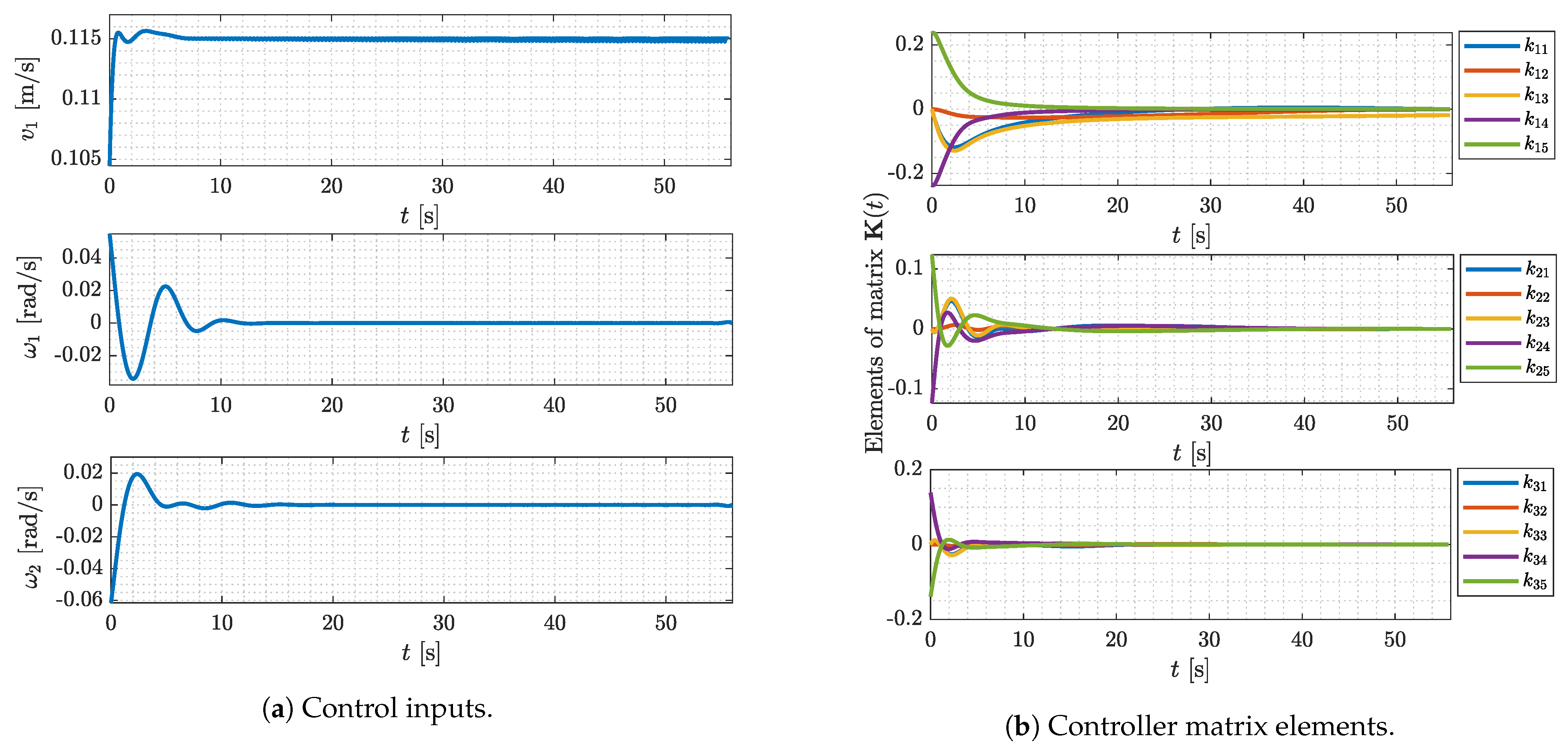
The simulation results of tracking a circular trajectory are shown in Figure 6 and Figure 7. The initial time is t 0 = 0 s, the final time is t f = 56 s and the number of optimization time intervals is N = 3500 . The initial positions and orientation angle of the robot are set to x ( t 0 ) y ( t 0 ) θ ( t 0 ) = 0 0 0 , while the initial steering angles are set according to Ackermann steering geometry as δ 1 ( t 0 ) δ 2 ( t 0 ) = arctan 2 a R arctan 2 a R , where a is the distance between the wheels (see Figure 1b) and R is the radius of the desired circle. The weight matrices Q and R of the objective function are chosen as Q = diag ( 10 4 , 1 , 10 3 , 1 , 10 4 ) and R = diag ( 10 2 , 10 6 , 10 6 ) .
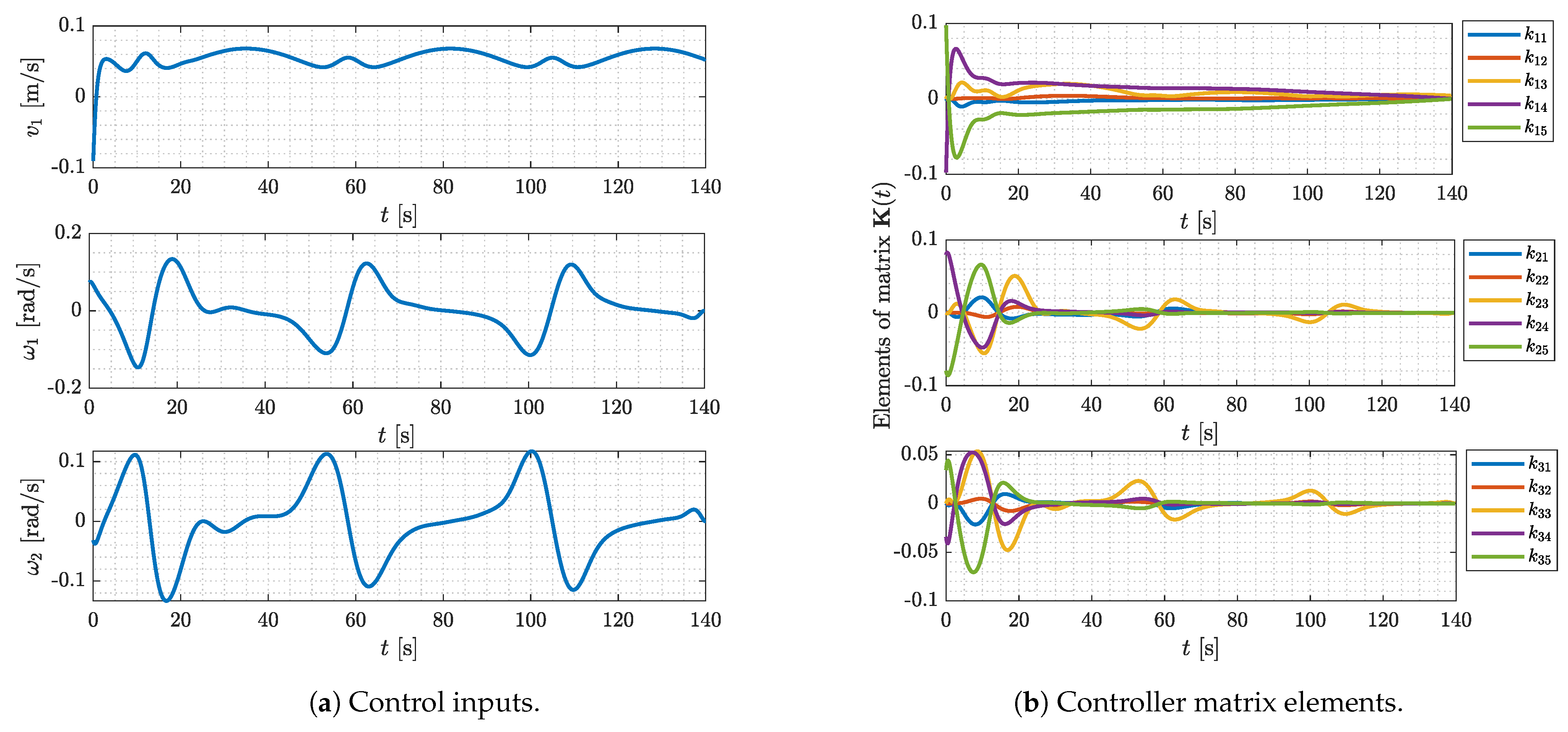
In Figure 6a, it can be seen that, due to quite precisely chosen initial conditions based on Ackermann’s formula, the robot instantly starts following the desired trajectory. The time responses of positions x and y, orientation angle θ , and steering angles δ 1 and δ 2 are shown in Figure 6b and Figure 6c, respectively. Furthermore, the time responses of control inputs, i.e., linear velocity v 1 and steering velocities ω 1 and ω 2 , are shown in Figure 7a. From their responses and maximum values, it can be seen that these velocities, as it was in the previous case of a straight line, are achievable on the actuators of the experimental set-up of the 4ISW4IAW mobile robot. The time dependencies of the elements of the state controller matrix calculated by the proposed algorithm in the case of a circular trajectory are shown in Figure 7b.

4.1.3. Curvilinear Trajectory Tracking

The desired curvilinear trajectory is defined as follows:
x d ( t ) = cos ω t 2 + sin 2 ω t 2 1 2 , y d ( t ) = cos 2 ω t 2 + sin ω t 2 3 5 , θ d ( t ) = atan 2 y ˙ d ( t ) , x ˙ d ( t ) ,
where ω = 2 π t f and t f is the final time. In order to obtain the reference of the robot, (67) together with (11)–(15) is included in (6)–(10), from which the desired robot states are calculated as follows:
x d 1 = cos ω t 2 + sin 2 ω t 2 1 2 , x d 2 = 4 sin 3 ω t 14 2 cos 4 ω t 12 cos 2 ω t + 9 sin ω t + 4 sin 5 ω t , x d 3 = arctan cos ω t 2 sin 2 ω t 2 cos 2 ω t sin ω t , x d 4 = cos ω t 4 cos ω t sin ω t 4 cos ω t 2 + sin ω t + 2 , x d 5 = cos 2 ω t 2 + sin ω t 2 3 5 ,
and the desired inputs are calculated as follows:
u d 1 = ω 4 sin ω t 2 + sin ω t 2 2 , u d 2 = 2 ω 17 cos ω t + 128 cos 5 ω t 2 cos 7 ω t 2 cos 4 ω t 12 cos 2 ω t + 9 sin ω t + 4 sin 5 ω t 2 2 ω 164 sin 2 ω t 38 sin 4 ω t 8 sin 8 ω t 2 cos 4 ω t 12 cos 2 ω t + 9 sin ω t + 4 sin 5 ω t 2 , u d 3 = ω 2 sin 3 ω t 7 4 sin ω t 2 + sin ω t 2 2 .
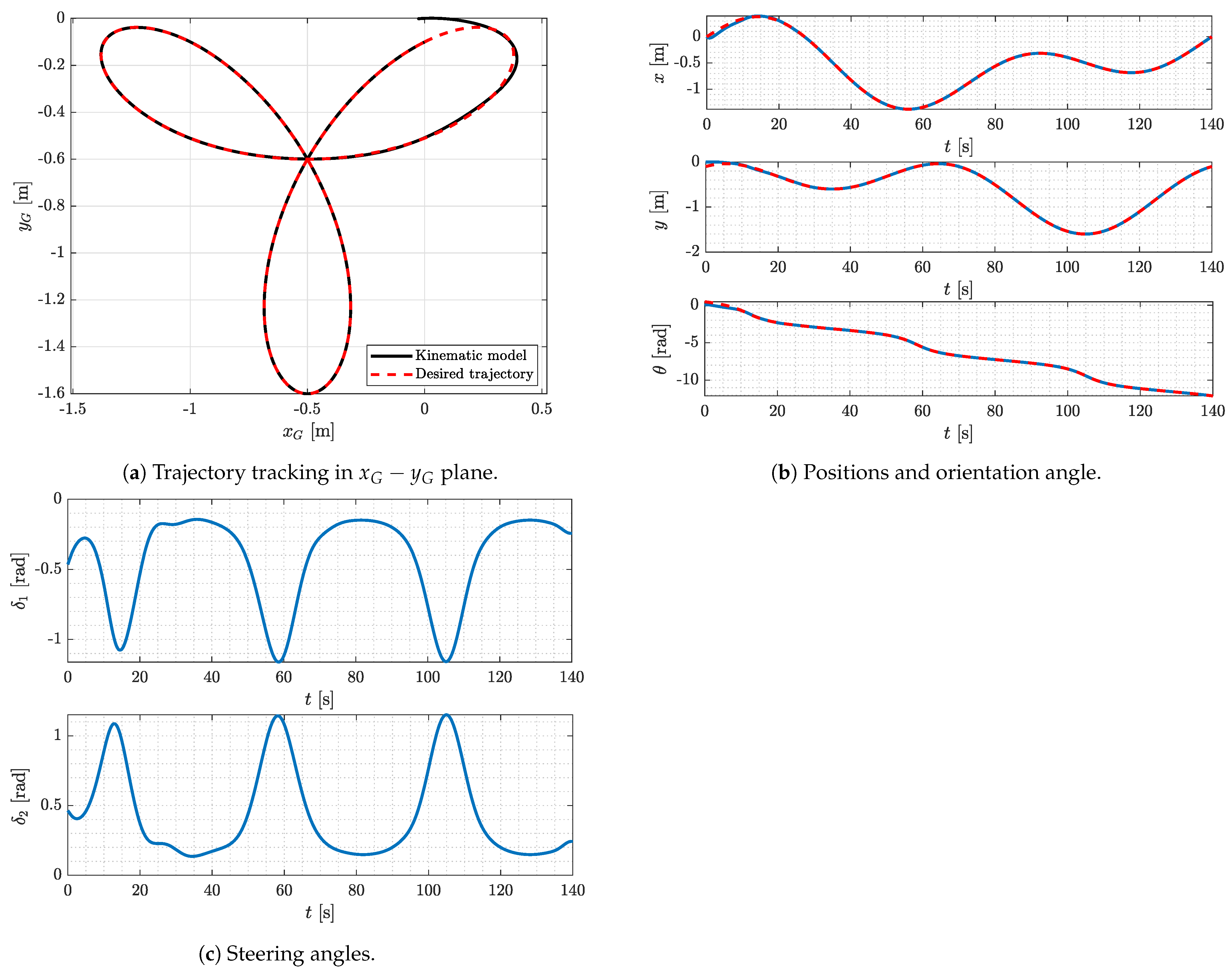
In Figure 8 and Figure 9, the simulation results of tracking a curvilinear trajectory are presented. The initial time is t 0 = 0 s, the final time is t f = 140 s and the number of optimization time intervals is N = 8750 . The initial positions and orientation angle of the robot are set to x ( t 0 ) y ( t 0 ) θ ( t 0 ) = 0 0 0 . In this case, the initial steering angles are chosen as δ 1 ( t 0 ) δ 2 ( t 0 ) = 0.46 0.46 . The weight matrices Q and R of the objective function are chosen as Q = diag ( 10 2 , 1 , 10 , 1 , 10 2 ) and R = diag ( 1 , 1 , 1 ) .
From Figure 8a, it can be observed that, after the transition from the initial conditions, the desired tracking is also achieved in this case of a curvilinear trajectory. In Figure 8b,c, the time responses of positions x and y, orientation angle θ , and steering angles δ 1 and δ 2 are shown. The time responses of control inputs, i.e., linear velocity v 1 and steering velocities ω 1 and ω 2 , can be seen in Figure 9a. It should be noted that the transition time from the initial conditions, the maximum values of control variables and the tracking accuracy can be further improved by appropriate adjustment of the weights in the Q and R matrices. This should be carried out in a manner that respects the limitations of the experimental robot system, i.e., it should involve seeking a balance with the desired response performance. The time dependencies of the elements of the state controller matrix calculated by the proposed algorithm are shown in Figure 9b.

4.2. Experimental Results

The objective of this subsection is to assess the efficacy of the previously developed control strategy within the context of the experimental set-up, which is detailed in Section 2.1. As mentioned earlier, the experimental set-up shown in Figure 1 was used to validate the control algorithm design.
The experiment is conducted in a way that the gains of the K ( t ) matrix are calculated in discrete time with a discretization time of 0.016 s, and the values are stored in a .dat file. A frequency of 62.5 Hz is chosen because the motor sampling time on the robot is set to this value, i.e., the motor states are sampled at this frequency. The robot control algorithm is executed on a standalone computer, and the velocity and steering angle values are sent via WiFi using ROS. The computer containing ROS and the robot with a single-board computer containing ROS are connected to a common WiFi network. The values are sent to the /trajectory topic, which contains a vector record of four velocities and four steering angles in the form [ v 1 , v 1 , v 1 , v 1 , δ 1 , δ 2 , δ 2 , δ 1 ] ; due to previously introduced conditions for switching to a chained form where the assumptions are made that all wheel velocities are equal ( v 1 ) , the front two wheels have the same steering angle ( δ 1 ) and the rear two wheels have the same steering angle ( δ 2 ) . Figure 10 shows a schematic of the laptop and the robot.
From Figure 10, it can be observed that the robot’s single-board computer collects data on the motor states (position, velocity and current) and stores them in the message type JointState and sending them to the laptop via the /joint_states topic. The sent motor states data is saved on the standalone computer using built-in rosbag modules and, upon completion of the experiment, the data is transferred to a .csv file for analysis and plotting. In the next section, the collected data from the experiment is shown together with a comparison to the reference and simulation data. More information regarding the previously mentioned ROS commands and functions can be found in the standard reference [38].
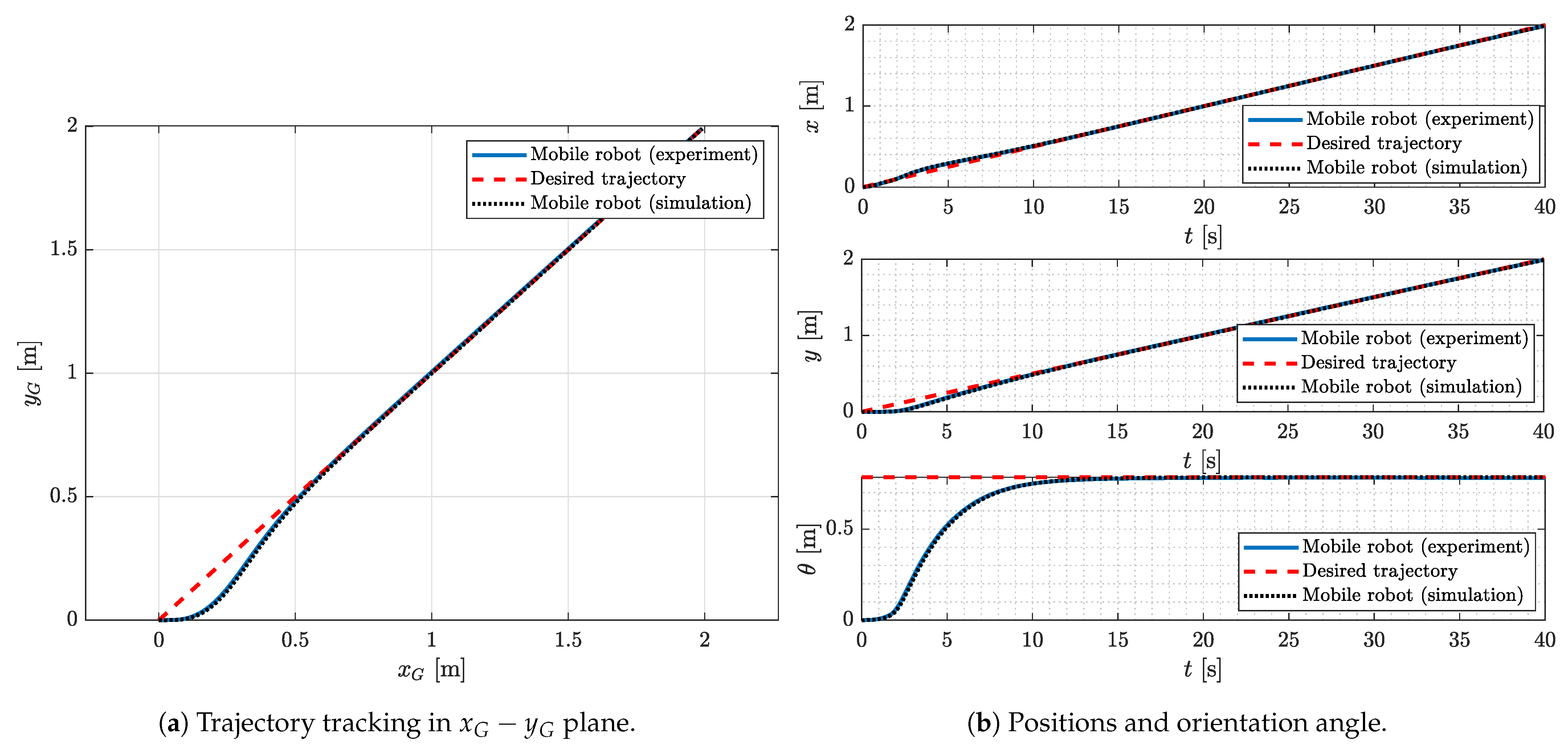
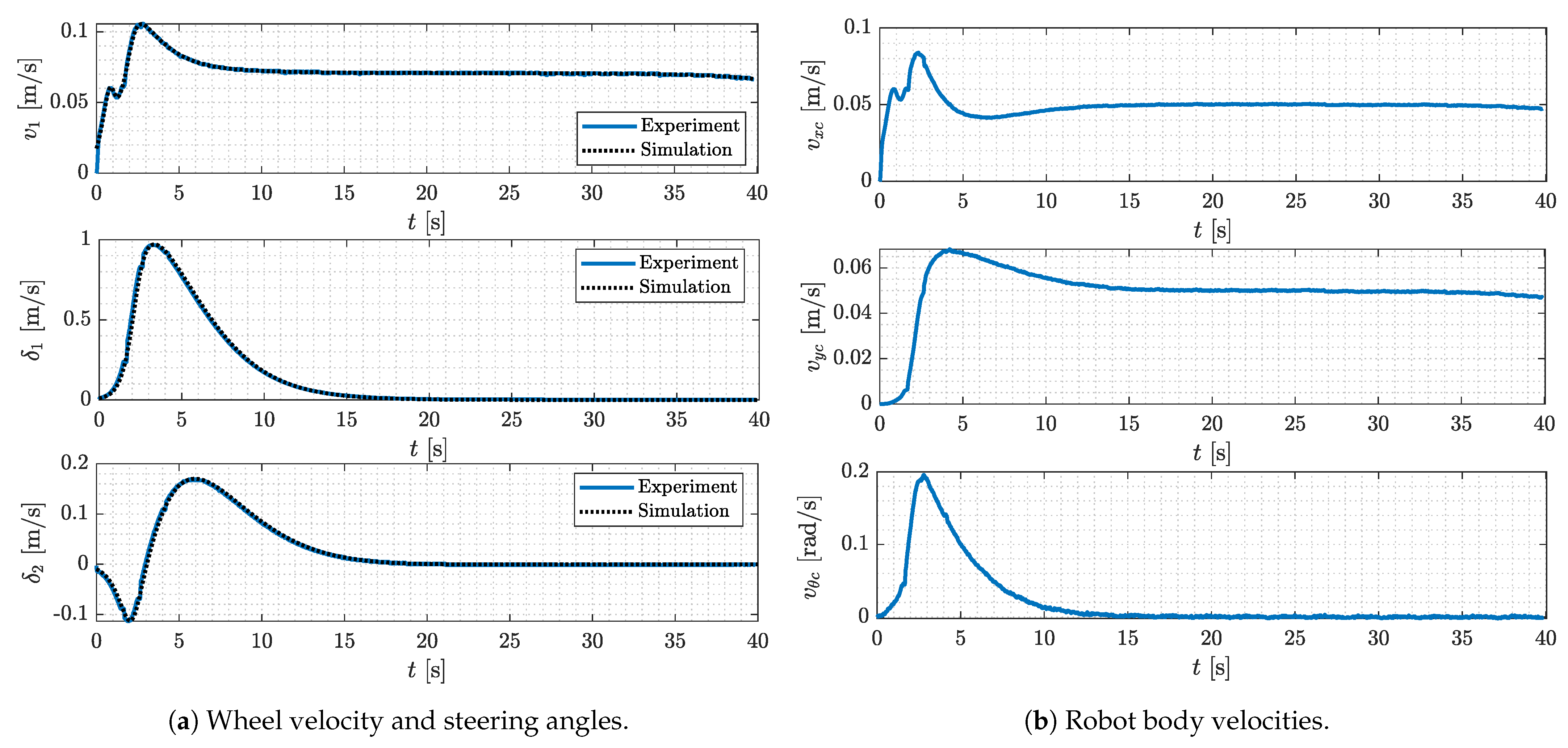
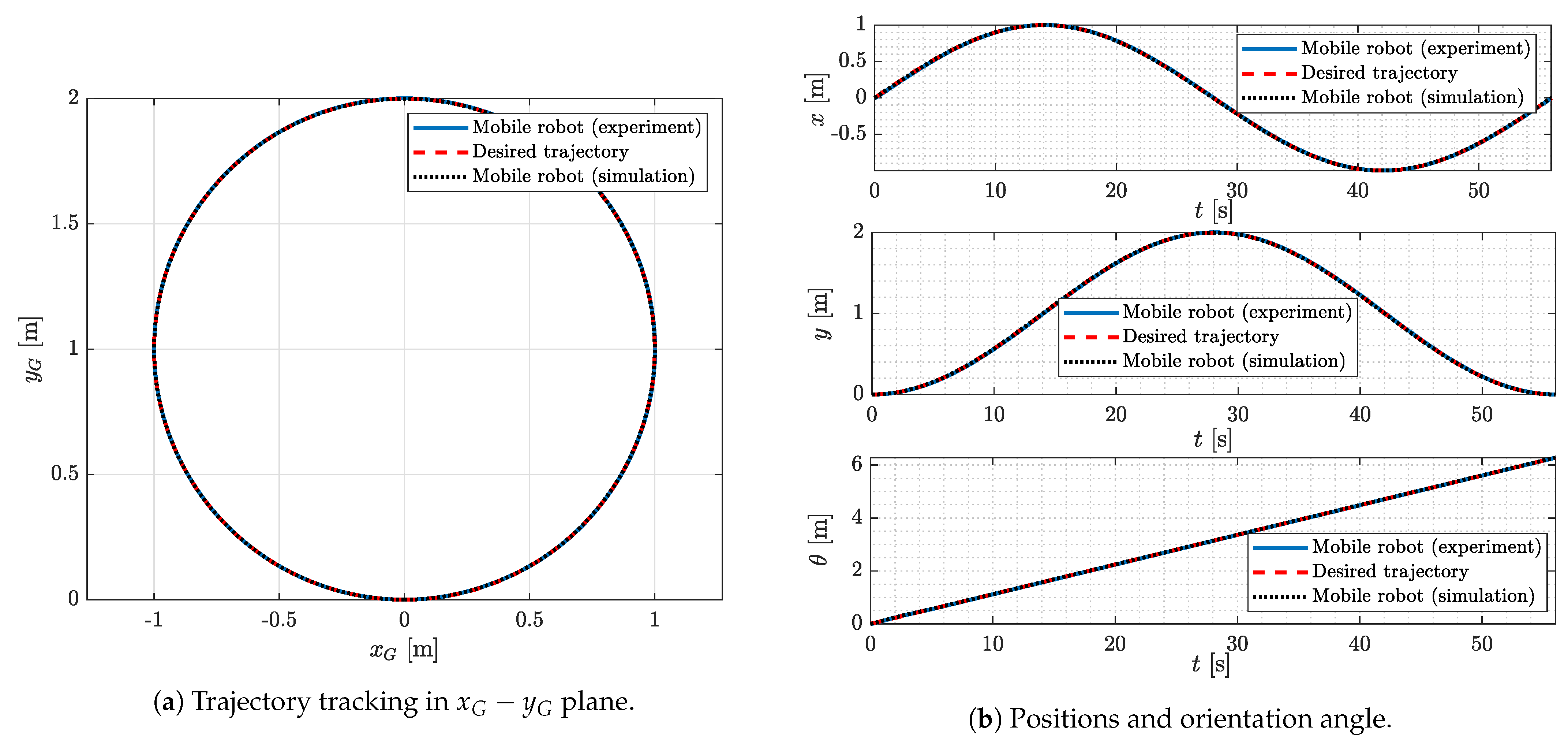
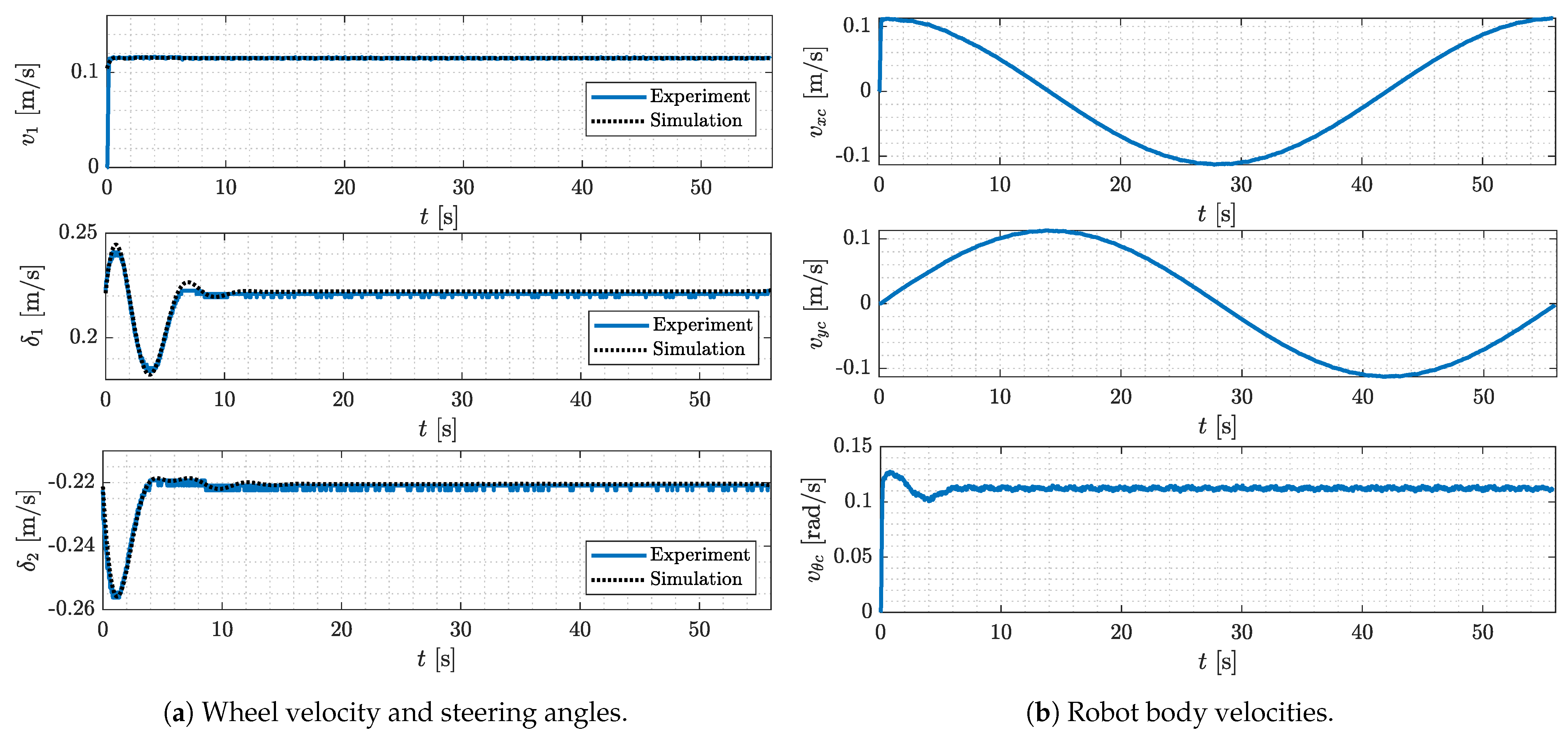
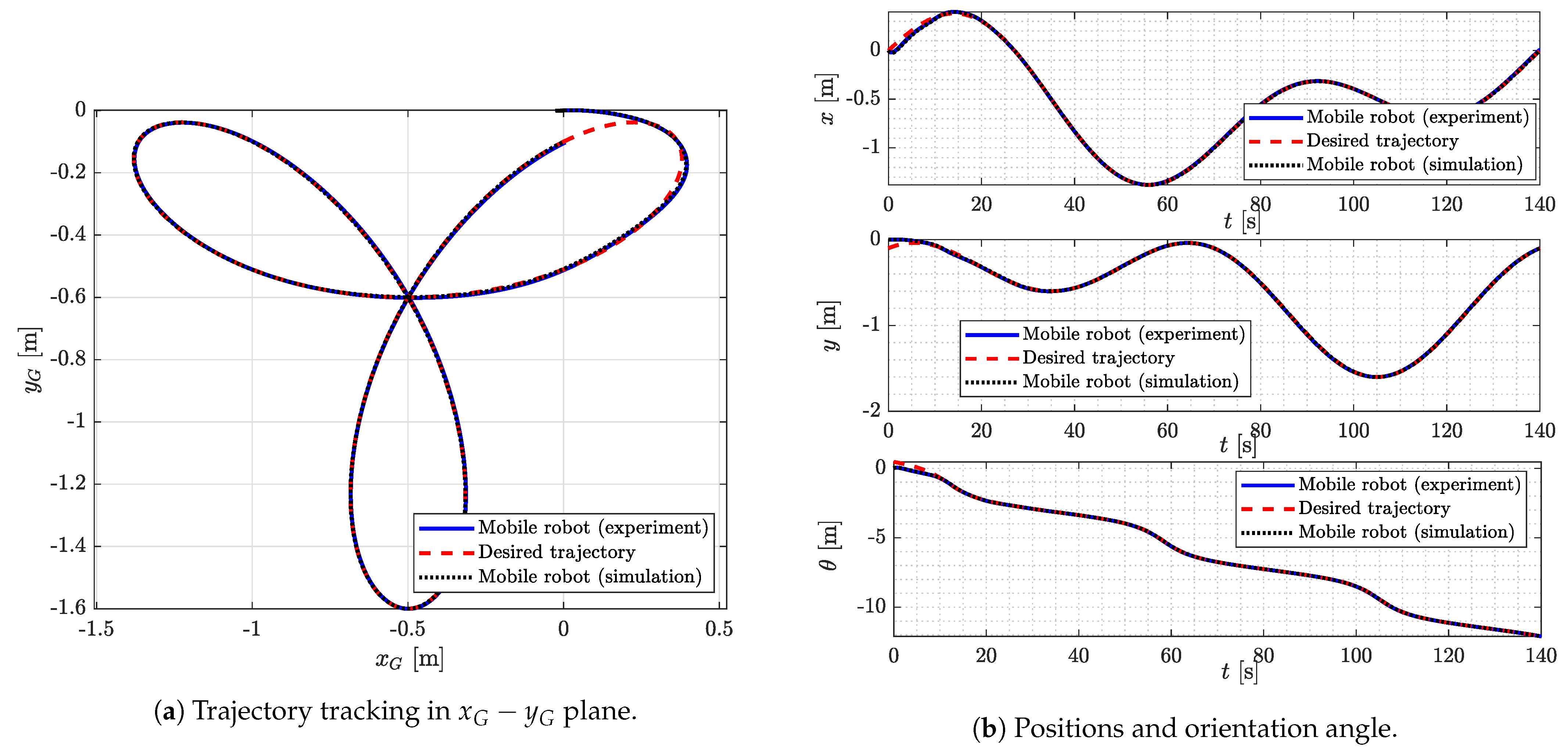
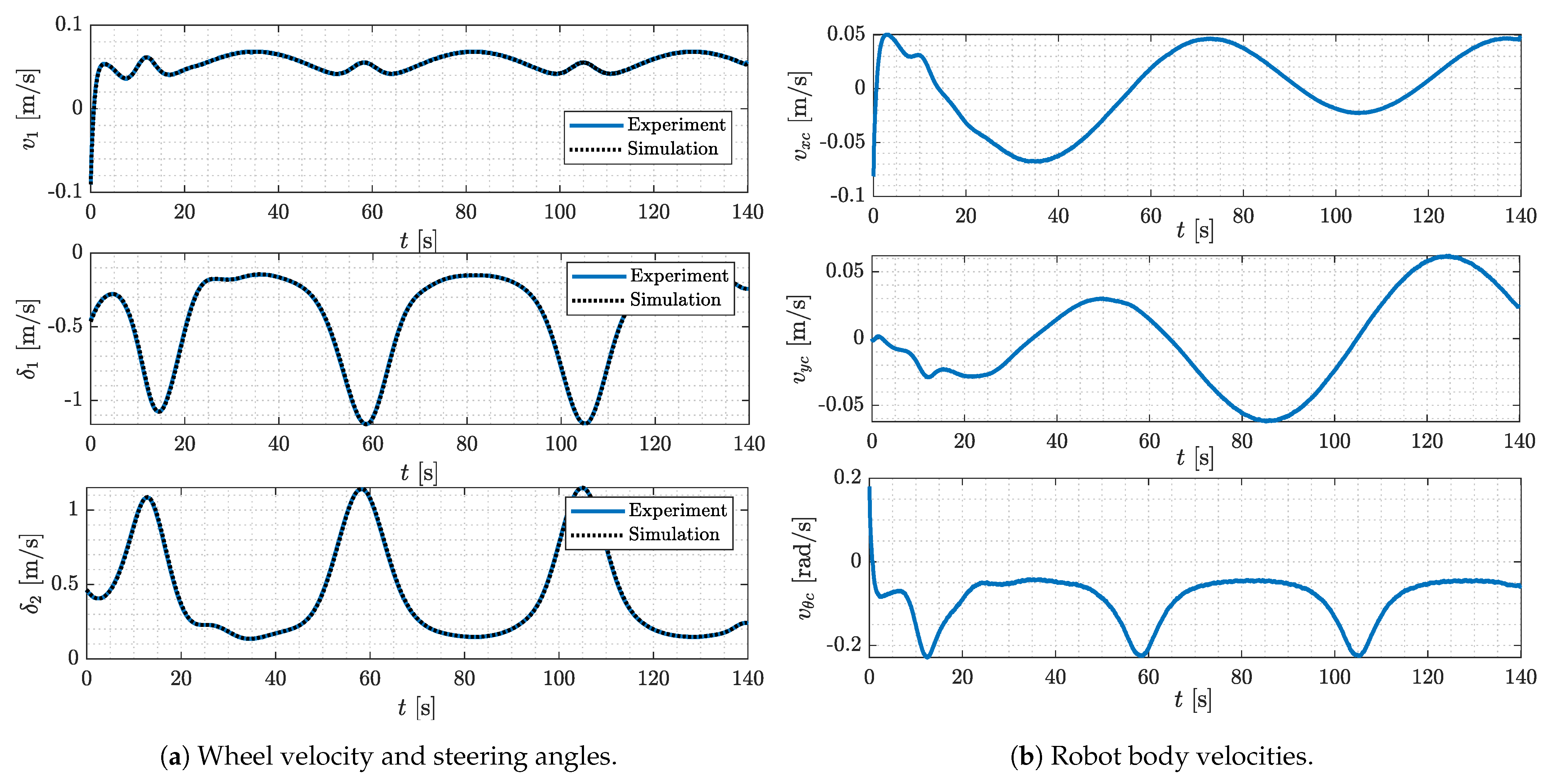
The results of the experimental validation of the proposed control strategy obtained from the data collected from the measuring system of the robot are shown in Figure 11, Figure 12, Figure 13, Figure 14, Figure 15 and Figure 16. The controller parameters and desired trajectory utilized in the experiment are the same as those selected and computed in the simulations.
Based on the presented experimental results, it can be concluded that, on the real system, by applying the proposed control strategy, a very good tracking accuracy of the desired trajectories is also achieved, as well as a fairly good match with the simulation results. Certain differences between the experimental and simulation results are caused by the eventual discrepancies in the values of the geometrical parameters of the robot that are used in the simulation from those that are real.
A closer examination of Figure 14a reveals the presence of oscillations in the steering angle responses. In order to achieve an optimal performance for trajectory tracking, it was necessary to implement high gains for the P controllers. However, if the gains were too high, oscillations were worse but tracking was better. The presented results demonstrate an optimal balance between good trajectory tracking for steering angles and smaller possible oscillations. Moreover, the implementation does not utilize a real-time kernel in Linux, resulting in a frequency of 62.5 Hz with an associated oscillation of approximately 1–2%. This oscillations may also be influenced by imperfections in the discretization time.
Furthermore, it should be mentioned that the presented results are obtained from the robot’s internal measurement system and, for a better insight into the robot’s positions and orientations in the global coordinate system, an external measurement system such as OptiTrack should be used. The application of this system will be included in future research.

4.3. Comparison with Other Methods

The main advantage of the approach proposed in this paper in comparison to other methods known to the authors for the design of a time-varying state controller for LTV systems is that it does not necessitate the iterative solution of the associated Riccati partial differential equation. This fact can be most effectively demonstrated in the context of tracking a circular trajectory. Upon examination of matrices A ( t ) and B ( t ) from Equation (60), it becomes evident that for the system to be fully controllable—which is the fundamental condition for solving the Riccati equation—it is necessary for u d 1 ( t ) to remain non-null throughout the time interval under consideration. From Equation (66), it is evident that u d 1 ( t ) is equal to zero for t = t f 4 , indicating that the system becomes uncontrollable. Consequently, the Riccati equation is unable to be solved or, at least, depending on the chosen discretization step, numerical issues may arise. It is evident from the presented simulations and experimental results that these problems do not arise in our approach.
Additionally, our approach avoids the computational complexity that can arise from the dimension of the LTV system. This is due to the structure of the procedure proposed for gradient calculation, which has a recursive time structure. In contrast, the Galerkin method of weighted residuals for solving Riccati differential equations has a cost that increases exponentially with the dimension of the LTV system. Furthermore, in comparison with the conventional numerical optimal control-based algorithms that employ penalty function methods or methods of Lagrange multipliers to obtain unconstrained formulations, the proposed algorithm is not constrained by high dimensions.
Compared to methods that use LMIs to solve the Riccati equation iteratively at each discrete time step, our approach requires fewer variables to be optimized. In this specific case of the control of a mobile robot, in our approach, due to the direct approach to the solution of the optimization problem, it is necessary to determine a total of 15 elements of the matrix K ( t ) . In the case of the application of LMIs, due to the bilinear dependence on the matrix K ( t ) , it would be necessary to introduce an appropriate substitution, which would extend the problem to the determination of a total of 29 optimization variables (it would be necessary to determine a symmetric positive definite matrix of dimension 5 × 5 and a matrix of dimension 3 × 5 ).
In comparison with the aforementioned methods, our approach has the limitation of lacking comprehensive recommendations for the initialization of specific algorithm parameters. This can been seen in the summarized steps of the algorithm presented in Section 3.2, where no particular guidance is provided on this matter. The initialization of these parameters directly affects the overall number of iterations required for convergence. LMI solvers are capable of converging with fewer iterations.
It should be noted that the algorithmic procedure presented in Section 3.2 is not intended for online calculation. The objective is to calculate the control law matrix as a function of time in an offline manner. It should be noted, however, that the overall control strategy depicted in Figure 3 is implemented in an online sense and also comprises the nonlinear equations of the chain model of the robot. Furthermore, the proposed strategy is easily programmable, as outlined in Section 4.2. While this paper has focused on the particular problem of mobile robot trajectory tracking, the proposed algorithmic optimization procedure has a number of applications in the context of the control of LTV systems. These include the assessment of system performance limits with different actuator configurations, the setting of realistic performance targets for online control systems and the tuning of parameters of online control systems.

5. Conclusions

In this paper, an approach to design a control system for a 4ISW4IAW mobile robot in a closed loop with a time-varying state controller, which has the goal of asymptotically following the desired trajectory, has been developed. In order to synthesize a controller, the three-input, two-chain, single generator chain model has been linearized in the vicinity of the desired trajectory into a system of control-oriented time-varying error equations.
An approach for the direct calculation of the time-varying state controller of LTV systems has been developed by combining several well-known techniques from the literature. This approach is an efficient algorithm that incorporates the conjugate gradient descent method, the line search method with Wolfe’s conditions, the Euler method for discretization and the chain rule for ordered derivatives, which were selected for their proven effectiveness.
In comparison with previous existing methods, the methodology presented in this paper offers two main advantages: firstly, it does not require the iterative solution of the corresponding Riccati partial differential equation; secondly, it has fewer optimization variables, which makes it more efficient. To the best of the authors’ knowledge, the application of the proposed approach for the synthesis of a 4ISW4IAW mobile robot control law has not yet been investigated.
A simulation and an experimental analysis of the proposed control strategy were performed on a real robot system. The results indicated that the applied control system was effective in following the desired trajectory with an acceptable degree of accuracy.
Future research could focus on the problem of position estimation. This can be accomplished by calibrating the kinematic parameters of the mobile robot, integrating an inertial measurement unit and tracking camera with an Extended Kalman Filter to obtain more accurate estimation.
In addition, future studies could be directed towards controlling both the robot’s dynamics and kinematics, whilst accounting for external disturbances and internal uncertainties inherent to the robot model. From the perspective of differential games, this class of problem can be regarded as one in which the control vector is the “player” that minimizes the optimality criterion, whereas the uncertainty/disturbance vector is the “player” that maximizes the optimality criterion—in other words, minimization and maximization must be carried out with respect to the same objective function. It should be noted here that the maximization of the performance criterion with respect to uncertainty/disturbance can be achieved simply by the change in sign in front of the gradient in the conjugate gradient method. Therefore, it is believed that the same principle of recursive calculation derived in this paper can be applied to the min–max control of LTV systems, thereby enabling the tracking of the desired trajectory of the 4ISW4IAW mobile robot. Furthermore, rather than assuming the initial positions of the 4ISW4IAW mobile robot are known a priori, it is possible to consider the case where the initial positions are treated as unknown uncertainty and the min–max multi-objective optimization problem should be solved.

Author Contributions

Conceptualization, B.Ć. and V.M.; methodology, B.Ć. and V.M.; software, B.Ć. and V.M.; validation, B.Ć., V.M., M.Š. and B.J.; formal analysis, B.Ć., V.M. and M.Š.; investigation, B.Ć., V.M. and M.Š.; resources, B.Ć., V.M., M.Š. and B.J.; data curation, B.Ć., V.M. and M.Š.; writing—original draft preparation, B.Ć. and V.M.; writing—review and editing, B.Ć., V.M., M.Š. and B.J.; visualization, B.Ć. and V.M.; supervision, M.Š. and B.J.; project administration, M.Š. and B.J.; funding acquisition, M.Š. and B.J. All authors have read and agreed to the published version of the manuscript.

Funding

The robot was funded by the European Union through the European Regional Development Fund’s Competitiveness and Cohesion Operational Program, grant number KK.01.1.1.04.0041, project “Autonomous System for Assessment and Prediction of infrastructure integrity” (ASAP).

Institutional Review Board Statement

Not applicable.

Informed Consent Statement

Not applicable.

Data Availability Statement

Data are contained within the article. Further inquiries can be directed to the corresponding author.

Acknowledgments

The authors would like to acknowledge the support of the project CRTA Regional Centre of Excellence for Robotic Technology, funded by the ERDF fund.

Conflicts of Interest

The authors declare no conflicts of interest.

Abbreviations

The following abbreviations are used in this manuscript:
4ISW4IAWFour Independently Steered Wheels and Four Independently Actuated Wheels
ASAAcrylonitrile Styrene Acrylate
DCDirect Current
LMILinear Matrix Inequality
LQRLinear Quadratic Regulator
LTVLinear Time Varying
PIDProportional–Integral–Derivative
PWMPulse-Width Modulation
ROSRobot Operating System
TVLQTime-Varying Linear Quadratic

References

  1. Tzafestas, S.G. Mobile Robot Control and Navigation: A Global Overview. J. Intell. Robot. Syst. 2018, 91, 35–58. [Google Scholar] [CrossRef]
  2. Rubio, F.; Valero, F.; Llopis-Albert, C. A review of mobile robots: Concepts, methods, theoretical framework, and applications. Int. J. Adv. Robot. Syst. 2019, 16, 1–22. [Google Scholar] [CrossRef]
  3. Alatise, M.B.; Hancke, G.P. A Review on Challenges of Autonomous Mobile Robot and Sensor Fusion Methods. IEEE Access 2020, 8, 39830–39846. [Google Scholar] [CrossRef]
  4. Fragapane, G.; de Koster, R.; Sgarbossa, F.; Strandhagen, J.O. Planning and control of autonomous mobile robots for intralogistics: Literature review and research agenda. Eur. J. Oper. Res. 2021, 294, 405–426. [Google Scholar] [CrossRef]
  5. Loganathan, A.; Ahmad, N.S. A systematic review on recent advances in autonomous mobile robot navigation. Eng. Sci. Technol. Int. J. 2023, 40, 101343. [Google Scholar] [CrossRef]
  6. Medina, L.; Guerra, G.; Herrera, M.; Guevara, L.; Camacho, O. Trajectory tracking for non-holonomic mobile robots: A comparison of sliding mode control approaches. Results Eng. 2024, 22, 102105. [Google Scholar] [CrossRef]
  7. Arab, A.; Hadžić, I.; Yi, J. Safe Predictive Control of Four-Wheel Mobile Robot with Independent Steering and Drive. In Proceedings of the 2021 American Control Conference (ACC), New Orleans, LA, USA, 25–28 May 2021; pp. 2962–2967. [Google Scholar]
  8. Liu, X.; Wang, W.; Li, X.; Liu, F.; He, Z.; Yao, Y.; Ruan, H.; Zhang, T. MPC-based high-speed trajectory tracking for 4WIS robot. ISA Trans. 2022, 123, 413–424. [Google Scholar] [CrossRef]
  9. Xie, Y.; Zhang, X.; Meng, W.; Zheng, S.; Jiang, L.; Meng, J.; Wang, S. Coupled fractional-order sliding mode control and obstacle avoidance of a four-wheeled steerable mobile robot. ISA Trans. 2021, 108, 282–294. [Google Scholar] [CrossRef] [PubMed]
  10. Jiang, L.; Wang, S.; Xie, Y.; Meng, J.; Zheng, S.; Zhang, X.; Wu, H. Anti-Disturbance Direct Yaw Moment Control of a Four-Wheeled Autonomous Mobile Robot. IEEE Access 2020, 8, 174654–174666. [Google Scholar] [CrossRef]
  11. Qiao, Y.; Chen, X.; Yin, D. Coordinated Control for the Trajectory Tracking of Four-Wheel Independent Drive–Four-Wheel Independent Steering Electric Vehicles Based on the Extension Dynamic Stability Domain. Actuators 2024, 13, 77. [Google Scholar] [CrossRef]
  12. Tan, X.; Liu, D.; Xiong, H. Optimal Control Method of Path Tracking for Four-Wheel Steering Vehicles. Actuators 2022, 11, 61. [Google Scholar] [CrossRef]
  13. Xu, Q.; Li, H.; Wang, Q.; Wang, C. Wheel Deflection Control of Agricultural Vehicles with Four-Wheel Independent Omnidirectional Steering. Actuators 2021, 10, 334. [Google Scholar] [CrossRef]
  14. Wu, H.; Li, Z.; Si, Z. Trajectory tracking control for four-wheel independent drive intelligent vehicle based on model predictive control and sliding mode control. Adv. Mech. Eng. 2021, 13, 1–17. [Google Scholar] [CrossRef]
  15. Dai, P.; Taghia, J.; Lam, S.; Katupitiya, J. Integration of sliding mode based steering control and PSO based drive force control for a 4WS4WD vehicle. Auton. Robot. 2018, 42, 553–568. [Google Scholar] [CrossRef]
  16. Dai, P.; Katupitiya, J. Force control for path following of a 4WS4WD vehicle by the integration of PSO and SMC. Veh. Syst. Dyn. 2018, 56, 1682–1716. [Google Scholar] [CrossRef]
  17. Božić, M.; Jerbić, B.; Švaco, M. Development of a Mobile Wall-Climbing Robot with a Hybrid Adhesion System. In Proceedings of the 2021 44th International Convention on Information, Communication and Electronic Technology (MIPRO), Opatija, Croatia, 27 September–1 October 2021; pp. 1136–1142. [Google Scholar]
  18. Božić, M.; Ćaran, B.; Švaco, M.; Jerbić, B.; Serdar, M. Mobile Wall-Climbing Robot for NDT inspection of vertical concrete structures. In Proceedings of the International Symposium on Non-Destructive Testing in Civil Engineering (NDT-CE 2022), Zurich, Switzerland, 16–18 August 2022; pp. 1–14. [Google Scholar]
  19. Bryson, A.E. Time-Varying Linear-Quadratic Control. J. Optim. Theory Appl. 1999, 100, 515–525. [Google Scholar] [CrossRef]
  20. Tedrake, R. Underactuated Robotics; MIT: Cambridge, MA, USA, 2023. [Google Scholar]
  21. Javadi, M.; Harnack, D.; Stocco, P.; Kumar, S.; Vyas, S.; Pizzutilo, D.; Kirchner, F. AcroMonk: A Minimalist Underactuated Brachiating Robot. IEEE Robot. Autom. Lett. 2023, 8, 3637–3644. [Google Scholar] [CrossRef]
  22. Vyas, S.; Maywald, L.; Kumar, S.; Jankovic, M.; Mueller, A.; Kirchner, F. Post-capture detumble trajectory stabilization for robotic active debris removal. Adv. Space Res. 2023, 72, 2845–2859. [Google Scholar] [CrossRef]
  23. Nortmann, B.; Mylvaganam, T. Direct Data-Driven Control of Linear Time-Varying Systems. IEEE Trans. Autom. Control 2023, 68, 4888–4895. [Google Scholar] [CrossRef]
  24. Ling, Y.; Wu, J.; Zhou, W.; Wang, Y.; Wu, C. Linear Quadratic Regulator Method in Vision-Based Laser Beam Tracking for a Mobile Target Robot. Robotica 2021, 39, 524–534. [Google Scholar] [CrossRef]
  25. Milić, V.; Di Cairano, S.; Kasać, J.; Bemporad, A.; Šitum, Z. A numerical algorithm for nonlinear L2-gain optimal control with application to vehicle yaw stability control. In Proceedings of the 2012 IEEE 51st IEEE Conference on Decision and Control (CDC), Maui, HI, USA, 10–13 December 2012; pp. 5040–5045. [Google Scholar]
  26. Milić, V.; Kasać, J.; Lukas, M. An Algorithm for Solving Zero-Sum Differential Game Related to the Nonlinear H Control Problem. Algorithms 2023, 16, 48. [Google Scholar] [CrossRef]
  27. Ćaran, B.; Švaco, M.; Šuligoj, F.; Jerbić, B. Modeling, Parameter Estimation and Control Design of 4WIS4WID Mobile Robot: Simulation and Experimental Validation. In Proceedings of the International Conference on Robotics in Alpe-Adria Danube Region, Cluj-Napoca, Romania, 12–14 June 2024; pp. 607–618. [Google Scholar]
  28. Lee, M.H.; Li, T.H.S. Kinematics, dynamics and control design of 4WIS4WID mobile robots. J. Eng. 2015, 2015, 6–16. [Google Scholar] [CrossRef]
  29. Ćaran, B.; Škifić, N.; Milić, V.; Švaco, M. Application of a Time-Varying Linear Quadratic Controller for Trajectory Tracking of a Four-Wheel Mobile Robot with Independent Steering and Drive. In Proceedings of the 2024 47th International Convention on Information, Communication and Electronic Technology (MIPRO), Opatija, Croatia, 20–24 May 2024; pp. 1–8. [Google Scholar]
  30. Tilbury, D.; Sordalen, O.; Bushnell, L.; Sastry, S. A multisteering trailer system: Conversion into chained form using dynamic feedback. IEEE Trans. Robot. Autom. 1995, 11, 807–818. [Google Scholar] [CrossRef]
  31. Walsh, G.; Bushnell, L. Stabilization of multiple input chained form control systems. Syst. Control Lett. 1995, 25, 227–234. [Google Scholar] [CrossRef]
  32. De Luca, A.; Oriolo, G.; Samson, C. Feedback control of a nonholonomic car-like robot. In Robot Motion Planning and Control; Springer: Berlin/Heidelberg, Germany, 1998; pp. 171–253. [Google Scholar]
  33. Fletcher, R.; Reeves, C.M. Function minimization by conjugate gradients. Comput. J. 1964, 7, 149–154. [Google Scholar] [CrossRef]
  34. Polak, E.; Ribiere, G. Note sur la convergence de mthodes de directions conjugues. Rev. Franaise D’inform. Et De Rech. Oprationnelle Srie Rouge 1969, 3, 35–43. [Google Scholar]
  35. Hestenes, M.R.; Stiefel, E. Methods of Conjugate Gradients for Solving Linear Systems. J. Res. Natl. Bur. Stand. 1952, 49, 409–436. [Google Scholar] [CrossRef]
  36. Dai, Y.H.; Yuan, Y. A Nonlinear Conjugate Gradient Method with a Strong Global Convergence Property. SIAM J. Optim. 1999, 10, 177–182. [Google Scholar] [CrossRef]
  37. Nocedal, J.; Wright, S.J. Numerical Optimization; Springer Science + Business Media, LLC: New York, NY, USA, 2006. [Google Scholar]
  38. Quigley, M.; Gerkey, B.; Smar, W.D. Programming Robots with ROS; O’Reilly Media: Boston, MA, USA, 2015. [Google Scholar]
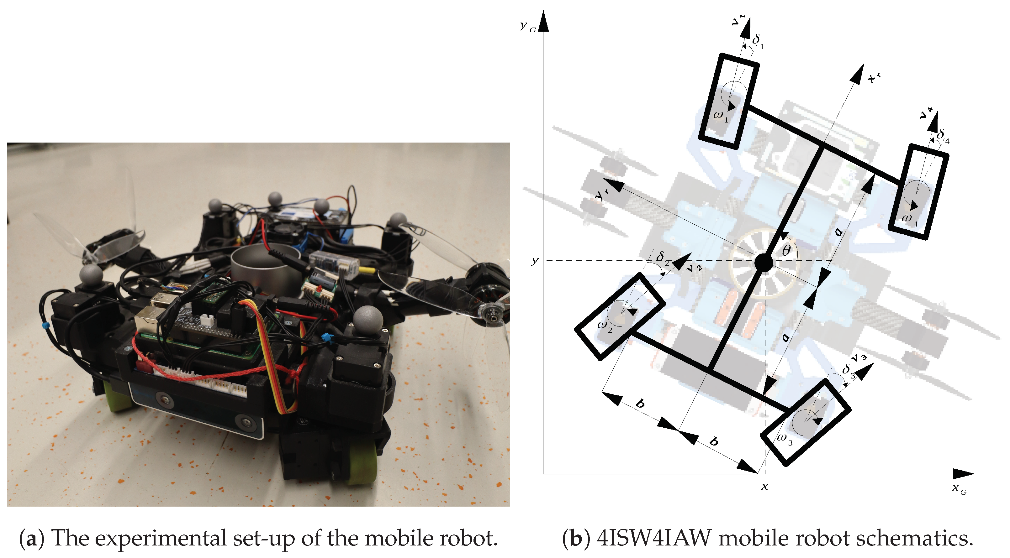
Figure 1. Photos of the experimental 4ISW4IAW mobile robot and kinematics schematics.
Actuators 13 00279 g001
Figure 2. Control schemes for driving and steering system of the mobile robot.
Actuators 13 00279 g002
Figure 3. Block diagram of the control strategy.
Actuators 13 00279 g003
Figure 4. Simulation results in the case of a straight line trajectory—positions, orientation and steering angles.
Actuators 13 00279 g004
Figure 5. Simulation results in the case of a straight line trajectory—linear and steering velocities, state controller matrix.
Actuators 13 00279 g005
Figure 6. Simulation results in the case of a circular trajectory—positions, orientation and steering angles.
Actuators 13 00279 g006
Figure 7. Simulation results in the case of a circular trajectory—linear and steering velocities, state controller matrix.
Actuators 13 00279 g007
Figure 8. Simulation results in the case of a curvilinear trajectory—positions, orientation and steering angles.
Actuators 13 00279 g008
Figure 9. Simulation results in the case of a curvilinear trajectory—linear and steering velocities, state controller matrix.
Actuators 13 00279 g009
Figure 10. Experimental set-up schematic.
Actuators 13 00279 g010
Figure 11. Experimental results in the case of a straight line trajectory—positions and orientation.
Actuators 13 00279 g011
Figure 12. Experimental results in the case of a straight line trajectory—robot velocities.
Actuators 13 00279 g012
Figure 13. Experimental results in the case of a circular trajectory—positions and orientation.
Actuators 13 00279 g013
Figure 14. Experimental results in the case of a circular trajectory—robot velocities.
Actuators 13 00279 g014
Figure 15. Experimental results in the case of a curvilinear trajectory—positions and orientation.
Actuators 13 00279 g015
Figure 16. Experimental results in the case of a curvilinear trajectory—robot velocities.
Actuators 13 00279 g016
Table 1. Steering and driving motor parameters.
R a Ω L a H K e Vs rad K m Nms rad b d Nms rad b s Nms rad J d [ kgm 2 ] J s [ kgm 2 ]
9.24 3 × 10 3 0.0103 0.0067 3.6 × 10 7 5.5 × 10 7 5 × 10 8 6 × 10 8
Table 2. Steering and driving motor parameters.
K vp K vi K pp K pi K pd ω n rad s
1.551140032.8
Disclaimer/Publisher’s Note: The statements, opinions and data contained in all publications are solely those of the individual author(s) and contributor(s) and not of MDPI and/or the editor(s). MDPI and/or the editor(s) disclaim responsibility for any injury to people or property resulting from any ideas, methods, instructions or products referred to in the content.