Article

Simulation Training System for Parafoil Motion Controller Based on Actor–Critic RL Approach

1
GNSS Research Center, Wuhan University, Wuhan 430072, China
2
Aviation Industry Corporation of China Aerospace Life Support Industries Ltd., Xiangyang 441003, China
3
School of Mechanical Engineering, Hubei University of Arts and Science, Xiangyang 441053, China
*
Author to whom correspondence should be addressed.
Actuators 2024, 13(8), 280; https://doi.org/10.3390/act13080280
Submission received: 19 June 2024 / Revised: 13 July 2024 / Accepted: 23 July 2024 / Published: 25 July 2024

Abstract

:
The unique ram air aerodynamic shape and control rope pulling course of the parafoil system make it difficult to realize its precise control. At present, the commonly used control methods of the parafoil system include proportional–integral–derivative (PID) control, model predictive control, and adaptive control. The control precision of PID control and model predictive control is low, while the adaptive control has the problems of complexity and high cost. This study proposes a new method to improve the control precision of the parafoil system by establishing a parafoil motion simulation training system that trains the neural network controllers based on actor–critic reinforcement learning (RL). Simulation results verify the feasibility of the proposed parafoil motion-control-simulation training system. Furthermore, the test results of the real flight experiment based on the motion controller trained by the proximal policy optimization (PPO) algorithm are presented, which are close to the simulation results.

1. Introduction

The parafoil system is a complicated, under-actuated system with the characteristics of strong cross-coupling, nonlinearity, and a large time delay and is easily affected by complex disturbances and intricate constraints [1]. The parafoil system can complete a left or right turn by pulling down the trailing edge of the parafoil [2]. Compared with helicopters, quadrotors, and fixed-wing unmanned aerial vehicles (UAVs), the parafoil system has poor maneuverability and is vulnerable to environmental influences because of its unique ram air aerodynamic shape and control rope pulling course. It is a big challenge for the parafoil system to achieve precise and stable motion control.
At present, the most reported literature on the parafoil control system concentrates on PID control, model predictive control, and adaptive control. The PID method is simple to implement, exhibits good stability, and offers reliable control performance, making it widely applied in the field of parafoil control. With the ecosystem particle swarm optimization (ESPSO) of the swarm intelligence optimization algorithm, the PID controller parameters’ tuning of the parafoil system has been achieved by Li et al. [3], and the effectiveness of the algorithm has been verified through simulation experiments. Another real-time model-independent control method for the parafoil system has been proposed by Zhao et al. [4,5] and is known as the model-free adaptive control (MFAC) method. Recently, the use of active disturbance rejection control (ADRC) has been introduced by Tao et al. [6,7], Sun et al. [8], and Jia et al. [9] to achieve precise control of the parafoil system. The ADRC utilizes an extended state observer (ESO) to estimate and compensate for system modeling errors and nonlinear uncertain disturbances. Compared to the PID method, both the MFAC and ADRC methods offer higher precision. However, the tuning of controller parameters is more challenging and can lead to issues such as oscillation and overshoot in certain situations.
Jagannath et al. [10] have comprehensively discussed how reinforcement learning (RL) is explored to provide autonomous control and navigation for unmanned devices, such as unmanned aerial vehicles (UAVs), unmanned ground vehicles (UGVs), and unmanned surface vehicles (USVs). Firstly, Polosky et al. [11] and Jagannath et al. [12,13] proposed a deep artificial intelligence neural network (AINN) to perform deep reinforcement learning (DRL). The AINN based on RL shows great potential in both aspects of automatic learning and complex nonlinear fitting, so it is capable of dealing with all kinds of complicated situations in motion control of the parafoil system. Chen et al. [14] exploited a muti-UAV autonomous path planning algorithm based on model-free reinforcement learning and introduced a hidden state of the recurrent neural network (RNN), which can solve the problem of incomplete information and low efficiency caused by partial observations and sparse rewards [15,16] in reinforcement learning and realize the multi-UAV cooperative autonomous path planning in an unknown environment. Zhao et al. [17] introduced parameter-sharing, off-policy, multi-agent path planning and the approach of using laser scan data as input based on the soft actor–critic (SAC) algorithm to guide the UAV to avoid obstacles and reach the goal. The simulation results proved the effectiveness of the presented approach in both the training process and task performance.
This study proposes a simulation training system for parafoil motion control using the actor–critic approach in reinforcement learning. The system explores a new approach to training parafoil controllers through reinforcement learning. The simulation training system consists of two main components. The one is a parafoil simulation environment, and the other is an actor–critic RL simulation training subsystem. The two components of the simulation training system operate independently of each other. The parafoil simulation environment comprises four modules: environmental factors (including aerodynamics [6,18], combined precise navigation, wind field simulation, actuator module [19,20], and trajectory planning [21,22]), as well as a performance-evaluation model, interaction model, and display model. The actor–critic RL simulation training subsystem includes two modules: parallel data sampling and the actor–critic reinforcement learning algorithm. The actor–critic [23] is a reinforcement learning approach, and different combinations of actor and critic can form different reinforcement learning algorithms. These algorithms offer significant advantages in handling complex tasks with continuous states and actions compared to traditional reinforcement learning algorithms. The objective of this study is to validate the feasibility of the proposed simulation training system based on the actor–critic approach, rather than to introduce a new and improved actor–critic algorithm. Therefore, for the subsequent experiments, the proximal policy optimization (PPO) algorithm [24] is selected, which is a recommended baseline algorithm by OpenAI. The PPO is a well-known actor–critic algorithm that exhibits stable performance and is easy to implement and tune. Although the latest actor–critic algorithms or significant optimizations of PPO are not employed, the controllers trained by the proposed simulation training system significantly outperform the traditional PID controllers.
This study is organized as follows: Section 2 illustrates the principle of the parafoil motion-control-simulation training system. Section 3 constructs a parafoil simulation environment. The parafoil motion-control-simulation training process is explained in Section 4. Simulation verification is performed in Section 5. A real flight test is conducted in Section 6. Finally, Section 7 presents the conclusions of this work.

2. Principle of the Parafoil Motion-Control-Simulation Training System

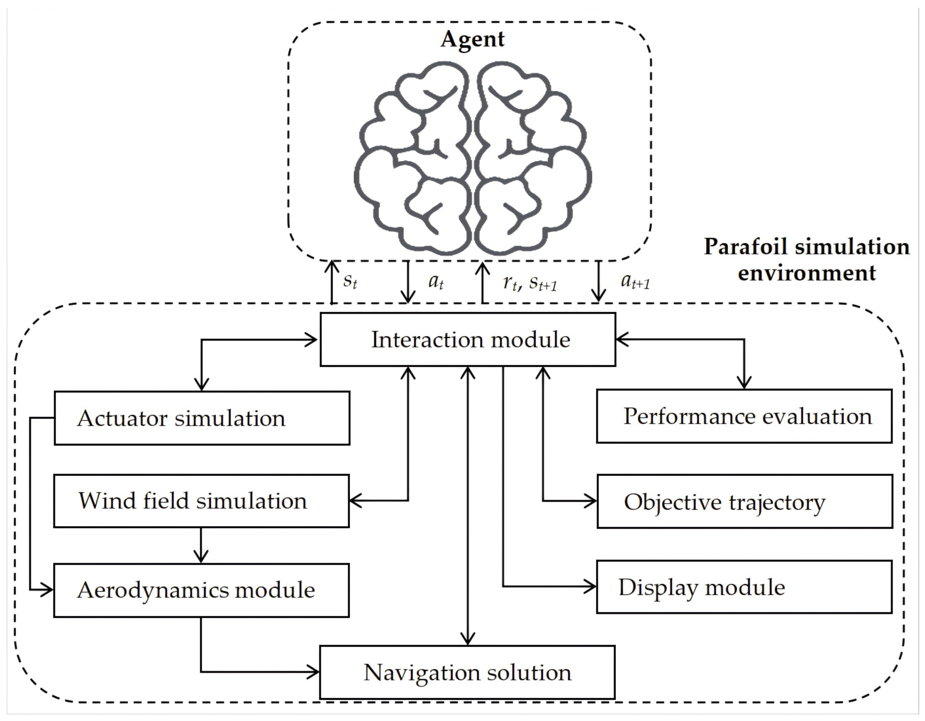
As depicted in Figure 1, the proposed parafoil motion-control-simulation training system includes the parafoil simulation environment and the actor–critic RL simulation training subsystem. The two parts execute the parafoil motion-control-simulation training through interaction with each other. The interaction process, a reinforcement learning (RL) loop, can be described below:
First, at time step t, the agent of the actor–critic RL simulation training subsystem observes a state st from the parafoil simulation environment and takes an action at based on the policy π(a|s) that maps state st (s = st) to action at (a = at);
Next, the parafoil simulation environment transitions into a new state st+1 and sends back a reward rt to the agent;
Then, a new training cycle of the agent is triggered, and the agent takes the next action at+1 to map with the state st+1;
Finally, the RL loop continues iteratively until the terminal state is reached and the episode ends.
The parafoil simulation environment contains four modules:
(1)
Environmental factors, composed of an aerodynamics module, navigation solution, wind field simulation, actuator simulation, and objective trajectory;
(2)
The performance-evaluation module, used to evaluate the trajectory-tracking performance and provide feedback on the performance evaluation information as a reward to the agent of the actor–critic RL simulation training subsystem;
(3)
The interaction module, employed to exchange information between the agent and the simulation environment;
(4)
The display module, used to display the objective trajectory and actual flight process of the parafoil.
Furthermore, the actor–critic RL simulation training subsystem includes two modules:
(1)
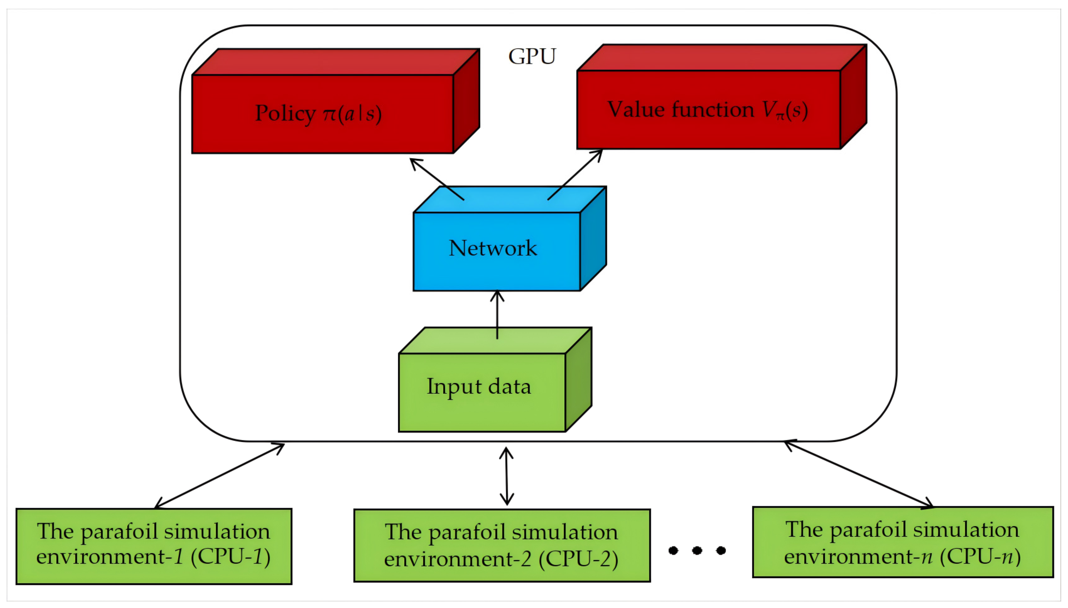
Parallel data sampling, utilizing one single GUP and multiple CPUs to speed up the parafoil motion-control-simulation training process;
(2)
Actor–critic reinforcement learning algorithm (Agent), using the data of the parallel data sampling to train the parafoil controller.
In summary, the whole simulation training system for the parafoil motion controller is developed using the Python (Python 3.9.5) language and run on a personal computer. Moreover, the parafoil environment simulation and the deep neural network-based agent training are operated on a server configured with a single GPU and multiple CPUs. The proposed simulation training system has three characteristics: first, the parafoil simulation environment is established based on the OpenAI-Gym standard. Second, part of the actor–critic RL algorithm is implemented using the OpenAI-RL open-source toolkit. Third, the deep neural network model is constructed and trained by the PyTorch open-source software (PyTorch 1.9).

3. Parafoil Simulation Environment

The parafoil simulation environment plays an indispensable role in realizing precise control of the parafoil system. The parafoil neural network motion-control training based on the actor–critic RL can only be executed in a simulation environment but not in a real scenario. There are two steps to create a precise control model for the parafoil system: first, generate an initial neural network control model by training in the simulation environment; second, adjust and optimize the control model by using some real data.
Figure 2 depicts the relationship among all the modules of the parafoil simulation environment, where st means the first state of the parafoil simulation environment provided to the agent, at is the first action of the agent mapping, st, st+1 represents the next state of the parafoil simulation environment, rt is the first reward given by the parafoil simulation environment to the agent, and at+1 means the next action of the agent mapping with state st+1. The calculation methods for state, action, and reward can be found in Appendix A, Appendix B and Appendix C.
These eight modules constituting the parafoil simulation environment in Figure 2 are exhibited below.

3.1. Interaction Module

The interaction module is the key module of the parafoil simulation environment. It mainly completes the following four functions: first, it receives the action from the trained agent; next, it simulates the action by coordinating with actuator simulation, wind field simulation, aerodynamics module, and navigation solution, and applies it to the parafoil. Then, it completes performance comparison and evaluation between the actual and objective trajectories. Finally, it collects state information from each module of the parafoil simulation environment and feeds it back to the agent.

3.2. Actuator Simulation

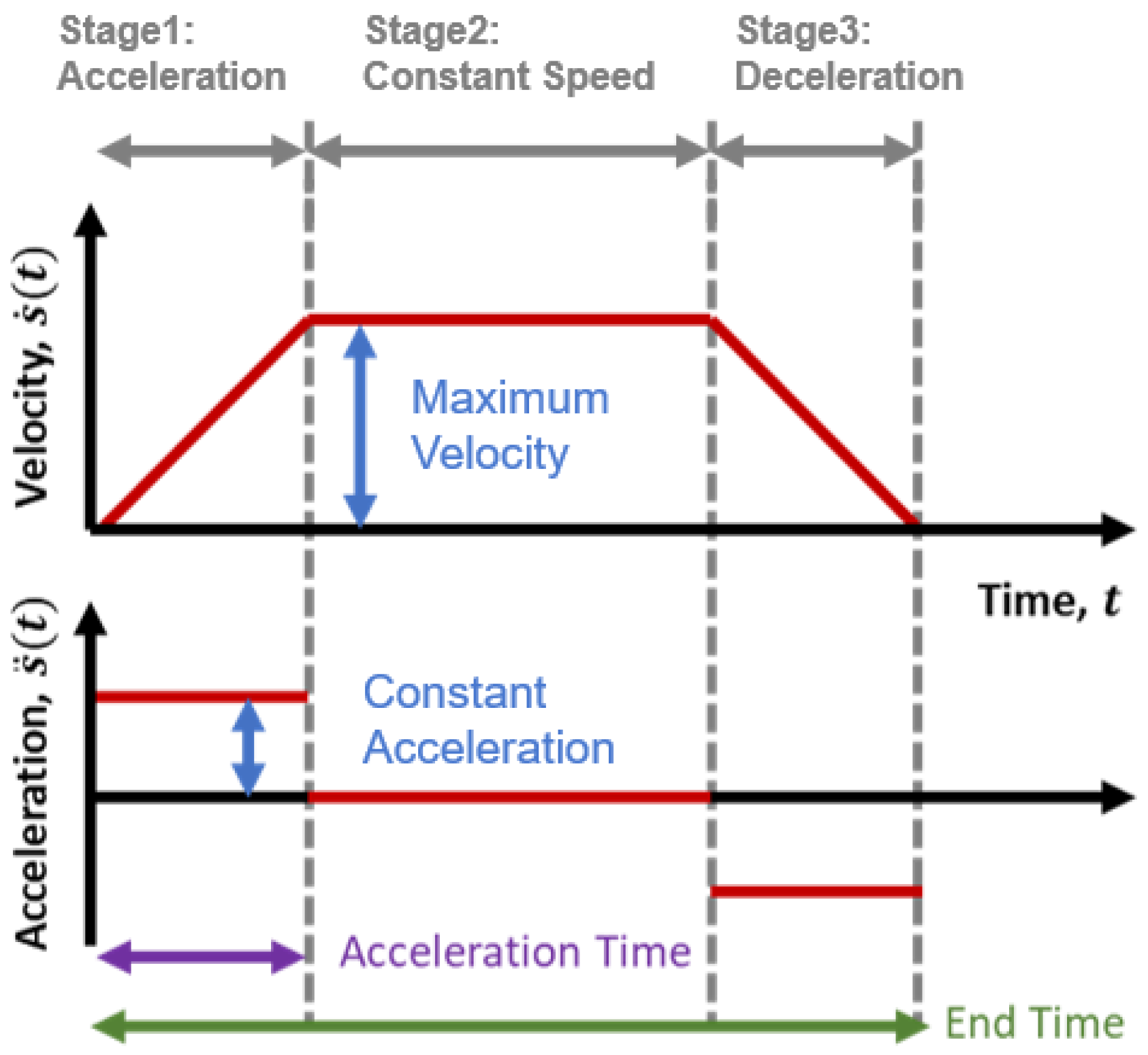
The actuator simulation in the parafoil simulation environment is applied to simulate the effect of a real motor pulling the control rope. The desired pulling length of the control rope is obtained by multiplying the control action with an inverse normalization constant (the maximum allowable length for pulling the control rope). The real parafoil system is constrained by the mechanical performance of the motor. When the motor receives the command to pull the control rope to the desired length, the motor begins to execute the command in the current state of the control rope. But the motor usually requires an execution process to complete the command (i.e., to pull the control rope to the desired length). To simulate this execution process in the parafoil simulation environment, this study designs the actuator simulation module, which uses a motor model constrained by a trapezoidal velocity profile [25]. The input of the actuator simulation is the desired pulling length of the control rope at a time t, and the output is the actual pulling length of the motor model, s(t), at the given time. The basic working principle of the motor constrained by the trapezoidal velocity profile is shown in Figure 3. Once the motor receives the command to achieve the desired length, it executes this command in three stages. (1) The Uniform Acceleration Stage: the motor accelerates at a constant rate until it reaches maximum speed. (2) The Constant Speed Stage: the motor continues to move at this maximum speed. (3) The Uniform Deceleration Stage: as the motor approaches the desired length, it decelerates at a constant rate until it stops.

3.3. Aerodynamics Module

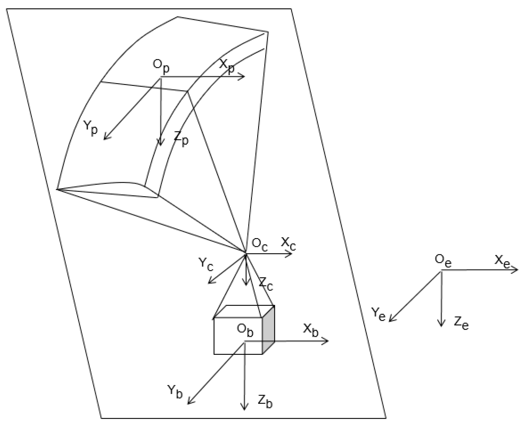
This study uses a 9-DOF model to describe the motion characteristics of the parafoil system and implements this model using Python (Python 3.9.5). The parafoil system is considered as a multi-rigid body composed of a rigid canopy and a rigid payload, with the canopy and payload connected by a spherical hinge, as shown in Figure 4. To establish the 9-DOF model, the following assumptions are made: (1) The length of the connecting rope remains unchanged. (2) The center of mass of the canopy overlaps with the center of aerodynamic pressure. (3) The payload’s lift is ignored, considering only the drag. Four coordinate systems are established to analyze the motion and forces of the parafoil system: the ground coordinate system OeXeYeZe, the parafoil canopy coordinate system OpXpYpZp, the payload coordinate system ObXbYbZb, and the parafoil system coordinate system OcXcYcZc. Then, the motion model of the parafoil system can be simplified to a three degrees of freedom translation from the connection point Oc and a three degrees of freedom rotation of the canopy and payload around point Oc. Therefore, a 9-DOF dynamic model of the parafoil system is established, and the kinematic equations are
x ˙ e y ˙ e z ˙ e = x ˙ c y ˙ c z ˙ c = u c v c w c
ϕ ˙ b θ ˙ b ψ ˙ b = 1 S ϕ b t θ b C ϕ b t θ b 0 C ϕ b S ϕ b 0 S ϕ b / C θ b C ϕ b / C θ b p b q b r b
ϕ ˙ p θ ˙ p ψ ˙ p = 1 S ϕ p t θ p C ϕ p t θ p 0 C ϕ p S ϕ p 0 S ϕ p / C θ p C ϕ p / C θ p p p q p r p
The dynamic equations are
M b R ~ c b 0 M b T b T b 0 M p + M F R ~ c p M p + M F T p T p I b 0 0 R ~ c b T b 0 I p + I F 0 R ~ c p T p Ω ˙ b Ω ˙ p V ˙ c F c = B 1 B 2 B 3 B 4
where
B 1 B 2 B 3 B 4 = F b A + F b G Ω ~ b M b Ω ~ b R c b F p A + F p G Ω ~ p M p + M F Ω ~ p R c p + M F Ω ~ p T p V c Ω ~ p M F T p V c M b A Ω ~ b I b Ω b M p A Ω ~ p I p + I F Ω p
The symbols in Equations (1)–(3) are defined as follows: Ti represents the transformation matrix from the inertial coordinate system to the other three coordinate systems, φi is the roll angle, θi is the pitch angle, ψi is the yaw angle, C * = cos(*), S * = sin(*), t * = tan(*), F * A is the aerodynamic force vector, F * G is the gravity vector, M * A is the aerodynamic moment vector, M * is the mass, I * is the moment of inertia, V * is the velocity, Ω * is the angular velocity, R * is the distance, and Ω ~ * and R ~ * represent their respective anti-symmetric matrices. In the subscripts, p represents the canopy, b represents the payload, c represents the connection point, and e represents the ground. The detailed modeling process can be referred to in [26,27,28,29].

3.4. Wind Field Simulation

The proposed wind field simulation is used to optimize the agent training by creating stationary and non-stationary wind speed models acting on the parafoil. Considering that the parafoil motion control is limited to a small space, the wind field simulation just simulates the local wind field of the parafoil’s current position. The complex and diverse local wind field can be realized by means of superposing several typical wind field models.
The proposed wind field in the parafoil simulation environment only discusses three typical wind fields: mean wind, random wind, and gust wind. The definitions of the three kinds of winds are introduced below:
(1)
First, in the application of the parafoil motion control, the mean wind is the main component of the wind field [30]. The mean wind means an average wind speed along the height over a period of time.
(2)
Next, the random wind can be seen as a kind of continuous stochastic pulses superposed on the mean wind. Both of its speed and direction vary randomly with time and location [19]. The magnitude of the random wind applied in this study is generated using a standard Gaussian distribution (with variance adjustable as needed), and the direction is generated using a uniform distribution in three-dimensional space.
(3)
Finally, the gust wind, caused by air disturbance, is a kind of special instantaneous wind with a speed of at least 5 m/s faster than the mean wind [31]. The proposed wind field in this study only discusses five basic gust winds: triangle gust wind, rectangular gust wind, half-wavelength gust wind, full-wavelength gust wind, and NASA gust wind [19,30]. In subsequent simulation experiments, only the widely used NASA gusts were employed. The mathematical model of the NASA gusts can be expressed as
V g u s t z = f N A S A z = V m a x 2 1 c o s π h z z 1 ,                                                               0 z z 1 < h V m a x   ,                                                                                                                                       h z z 1 < 2 d m h V m a x 2 1 c o s π h z z 1 2 d m ,               2 d m h z z 1 < 2 d m
where z is the current altitude, z1 is the position where the gust starts, Vmax is the maximum amplitude of the gust, dm is the half-thickness of the gust layer (ranging from 25 to 150 m), and h is the thickness of the atmospheric layer where the wind speed of the trapezoidal gust increases from 0 to Vmax at the front and rear edges.
The resultant wind vector W can be defined as
W = VWDW
where VW is a wind speed scalar, and DW represents a wind direction vector. DW is determined by the angles (α, β, γ) between the wind speed vector and the three axes (X, Y, Z) of the geodetic coordinate system.
The wind direction vector DW can be depicted as
D W = cos α cos β cos γ
Considering that the resultant wind in the wind field simulation is composed of the mean wind, the random wind, and the gust wind, the resultant wind vector W can also be written as
W = Wmean + Wrand + Wg
where Wmean represents the mean wind vector, Wrand represents the random wind vector, and Wg is the gust wind vector.

3.5. Navigation Solution

Figure 5 illustrates the navigation solution of the parafoil simulation environment. First, according to the current state (position of the connection point Oc, velocity of the point Oc, angular velocity of the canopy and payload, Euler angles (yaw, pitch, and roll) of the canopy and payload, wind speed, and control quantity) of the parafoil, the current acceleration, angular acceleration, and Euler angular velocity can be obtained by solving the aerodynamic model. Second, the next state (position of the connection point Oc, velocity of the point Oc, angular velocity of the canopy and payload, Euler angles (yaw, pitch, and roll) of the canopy and payload) of the parafoil can be calculated by the integration algorithm.

3.6. Objective Trajectory

The basic principle of the trajectory-planning algorithm is to experience as few complex situations as possible and perform the simplest control actions, which is totally opposite to the aim of the parafoil motion-control-simulation training. Thus, the normal trajectory-planning algorithms do not apply in obtaining the parafoil objective trajectories for the parafoil motion-control-simulation training.
This study introduces a simple and novel method, the simulated flight, to work out the parafoil objective trajectories. Each simulated flight will obtain a flying trajectory used as an objective trajectory in this study. By setting different initial states of the parafoil system, wind field, and control sequence for the simulated flight, this study obtains a large amount of complex objective trajectories. The specific method for generating the objective trajectory can be found in Appendix D.

3.7. Performance Evaluation

The performance evaluation of the parafoil objective trajectory tracking control includes four aspects: distance error, direction error, control stability, and power dissipation [1]. The four performance indexes are packaged as a reward signal and transmitted to the agent. This study only uses the most important performance index of distance error and leaves the other indexes for future work.

3.8. Display Module

For ease of observing the parafoil flight, debugging, and evaluating the parafoil motion-control-simulation training, this study uses Matplotlib (Matplotlib 3.3.2) to show the parafoil flight trajectory. The Matplotlib has two display modes: real-time and non-real-time displays. In the real-time display mode, both the parafoil flight trajectory and motion-control-simulation training process can be seen in the Matplotlib. Otherwise, only the result of the parafoil motion-control-simulation training can be observed.

4. Actor–Critic RL Simulation Training Subsystem

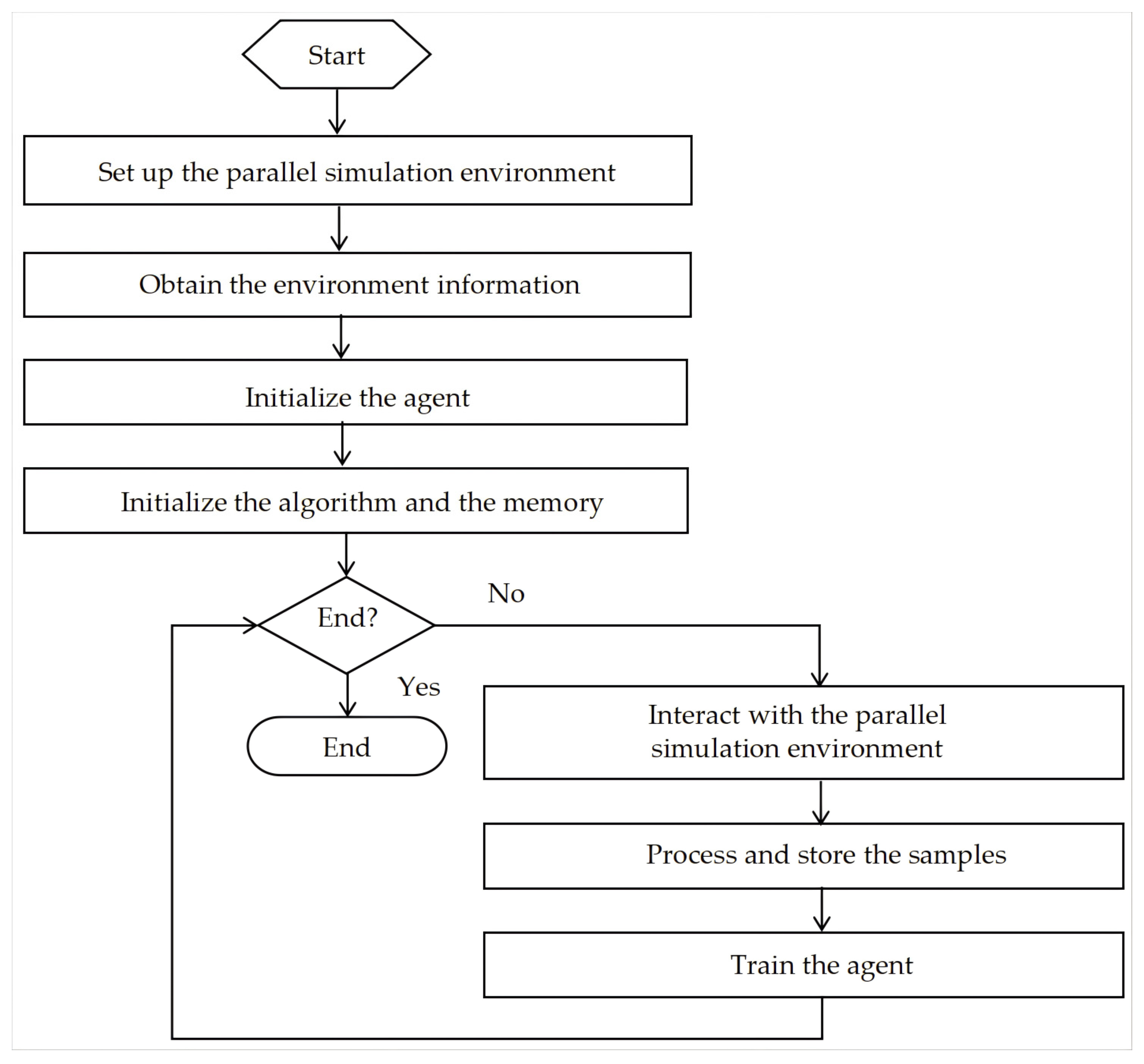
Section 2 stated that the parafoil motion-control-simulation training subsystem is composed of a parallel data sampling module and actor–critic reinforcement learning algorithm (Agent). Figure 6 shows the work flowchart of the parafoil motion-control-simulation training. To improve the sampling efficiency, the parafoil motion-control-simulation training subsystem applies the parallel mode to interact with the parafoil simulation environment. During the parallel sampling, different simulation environments are independent of each other.

4.1. Parallel Data Sampling

Training the parafoil neural network motion controller using reinforcement learning (RL) calls for a large number of parafoil trajectory samples to be obtained by interaction between the agent and the parafoil simulation environment. However, the interaction that occurred between the agent and the single simulation environment sample is time-inefficient. For example, in the on-policy RL training, it takes about ten seconds (10 s) to generate a one-hundred-second flight trajectory by a single sample interaction. In this case, if not considering the agent training time but the sample acquisition time, it takes about 2777.7 h to perform one-million-time parafoil neural network motion-control training, which is totally unacceptable in real operation. So, this study introduces a parallel sampling of multiple simulation environments. Figure 7 shows that the parafoil neural network motion-control training consists of n sub-processes and one host process. In addition, the RL algorithm used for the parafoil motion-control training contains two primary functions of policy π(a|s) and value function (s). “s” and “a”, respectively, represent the simulation environment state and the action of the agent at time t. Each sub-process means one independent simulation environment sampling run by one CPU. The host process contains the tasks of interacting with all the simulation environments, collecting the interaction samples (“Input data” in Figure 7), and training the parafoil neural network motion controller based on GPU. The multiprocessing.Pipe (“Network” in Figure 7) method is employed to transfer data between the sub-processes and the host process.

4.2. Actor–Critic Reinforcement Learning Algorithm

The actor–critic approach utilized in the parafoil motion-control-simulation training is a type of reinforcement learning method that learns both policy and value functions [23]. This method excels in handling complex tasks with continuous states and continuous actions. As depicted in Figure 8, the general structure of the actor–critic approach consists of an actor model and a critic model [24,32,33]. The actor model does not directly receive the reward signal, while the critic model does not directly select the corresponding actions. The actor model learns policies using the Monte Carlo policy gradient, while the critic model learns the value function using a temporal difference algorithm. The entire learning process involves the following steps: first, the critic model generates a temporal difference error δ by utilizing the reward signal and the current estimation of values, and it updates its model parameters accordingly; second, the actor model calculates the policy gradient based on the values estimated by the critic model and adjusts its own policy using the policy gradient.
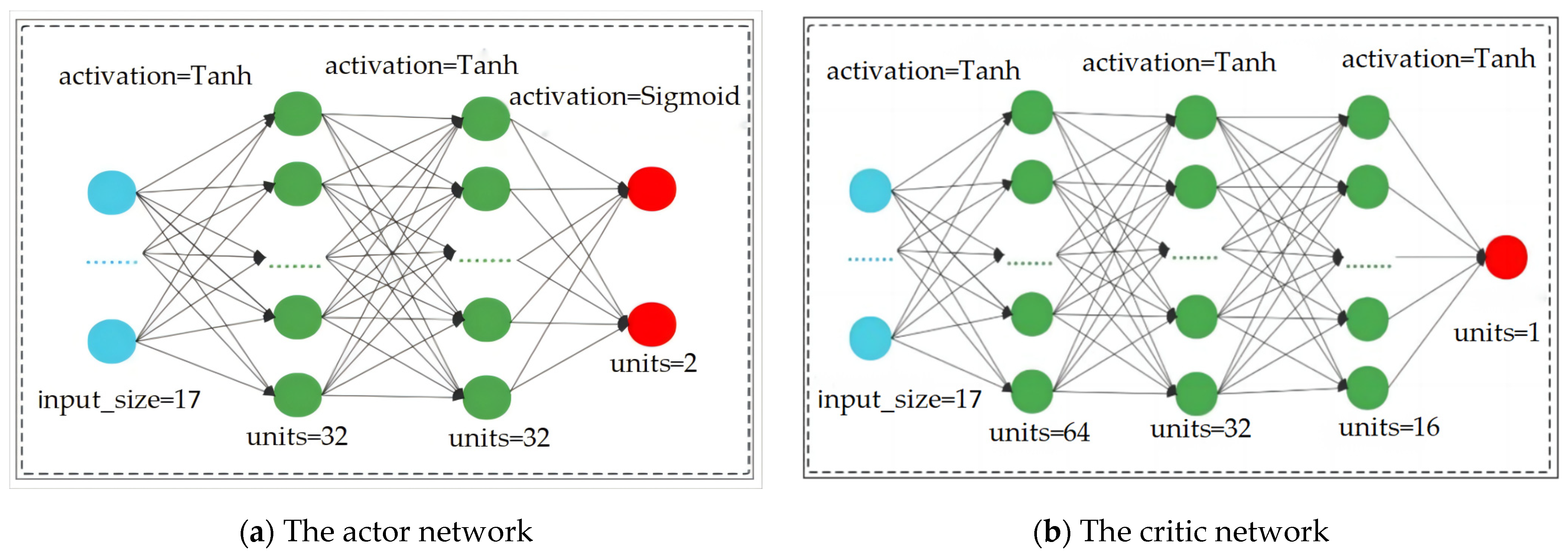
In this study, the proximal policy optimization (PPO) algorithm (a typical actor–critic algorithm) is employed. It is compatible with parallel data sampling, is easy to implement, and exhibits stable performance. Figure 9 illustrates the network structure of the PPO algorithm. The graph in Figure 9a represents the actor network structure, and that in Figure 9b is the critic network structure.

5. Simulation Verification

5.1. Parafoil Motion-Control-Simulation Training Procedure

Figure 10 shows the parafoil motion-control-simulation training procedure. The parafoil simulation environment parameters mainly include the parafoil geometry size and mass parameters, aerodynamic parameters, model freedom, payload, etc. The reinforcement learning (RL) parameters consist of the RL algorithm, neural network model, learning rate, discount factor, replay buffer size, etc. The objective task parameters contain the parafoil initial state, objective trajectory, task runtime, observation state, output action, task reward, etc. The environmental conditions are composed of wind field and observation noise. The parallel simulation environment contains the parafoil simulation environment samples, update frequency, sampling frequency, etc.

5.2. Performance Index

Let HDE(z) denote the horizontal distance error between a point in real trajectories of the parafoil and the corresponding point in objective trajectories at the same altitude z. This study uses the indexes below to measure the performance of parafoil motion controllers.
maxHDE: the max HDE(z) in a single-flight task;
meanHDE: the mean HDE(z) in a single-flight task;
stdHDE: the standard deviation of the HDE(z) in a single-flight task;
max_maxHDE: the max maxHDE in N flight tasks;
mean_meanHDE: the mean meanHDE in N flight tasks;
mean_stdHDE: the mean stdHDE in N flight tasks.

5.3. Analysis of the Parafoil Motion-Control-Simulation Training Results

5.3.1. Influence of Hyper-Parameter Settings on Reinforcement Learning Training

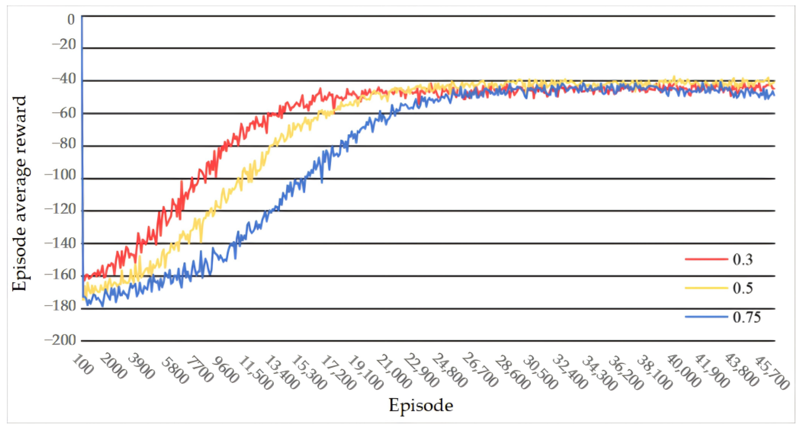
During the whole reinforcement learning (RL) training, the “TensorBoard” can be used to observe how the different hyper-parameter settings change RL training. Figure 11 and Figure 12, respectively, exhibit the influence of the initial values of standard deviation for the sampling and learning rate on the RL training.
One important challenge the standard deviation settings for sampling must face is the trade-off between exploration and exploitation. “Exploration” means the agent has to explore in order to make better action selections in the future. “Exploitation” represents the agent having to exploit what it has already experienced in order to obtain a reward. It is not possible to explore and exploit in a single action selection, and the agent often refers to the conflict between exploration and exploitation. Compared with exploitation, the reward is lower in the short run but higher in the long run during exploration.
Figure 11 shows that the highest growth rate of the episode average reward is obtained when the initial value of the standard deviation parameter equals 0.3, the lowest growth rate is obtained when the initial value is 0.75, and the optimal convergence performance of the episode average reward is acquired when the initial value is 0.5. So, it can be concluded from Figure 11 that the larger the value of the standard deviation for sampling is, the more likely the agent is to pursue exploration. Contrarily, the more likely the agent is to choose exploitation. Reinforcement learning requires a balance between exploration and exploitation.
Figure 12 shows that during the early stage of the training process, the bigger the initial value of the learning rate is, the higher the growth rate of the episode average reward is. However, a bigger value of the learning rate does not mean a better convergence performance of the episode average reward curve. In conclusion, a more rewarded and stable training model can be obtained by setting a moderate learning rate.

5.3.2. Control Effect Comparison between PID and PPO Parafoil Motion Controllers

The test simulation experiments of the two parafoil motion controllers individually based on PID (proportional–integral–derivative) and PPO (proximal–policy–optimization) are presented. The tested PID parafoil motion controller is a traditional PID controller, which is widely used in engineering due to its ease of implementation. The input information for the PID controller is the deviation between the desired and actual heading angles, as well as the integral and differential variants of this deviation, with the output being the control action. Its parameters usually require expert tuning or can be set using intelligent algorithms such as the swarm intelligence optimization algorithm. The PID controller parameters used in this study were tuned by experts in a parafoil simulation environment, with values set to Kp = 0.72, Ki = 0.002, and Kd = 0.90. The tested PPO parafoil motion controller, based on actor–critic type reinforcement learning (RL), is a parafoil neural network motion controller trained by the simulation training system introduced in this study. The multi-layer perceptron (MLP) of the proposed PPO parafoil motion controller is composed of the input layer (17 × 64, ReLu), the first hidden layer (64 × 32, ReLu), the second hidden layer (32 × 16, ReLu), and the output layer (16 × 1, Sigmoid).
The test collection of the parafoil objective trajectories consists of 100 randomly generated trajectories. The parafoil flights from the start point of the objective trajectories. The PID and PPO parafoil motion controllers perform 300-step controls in continuous time; record the comparison results of objective and flight trajectories; and calculate the maximum, average, and variance of the horizontal distance error between the parafoil objective and real trajectories. The test simulation experiments include two parts: first, the single flight comparison between the parafoils based on PID and PPO. Second, the multiple flights.
(1)
Single Flight
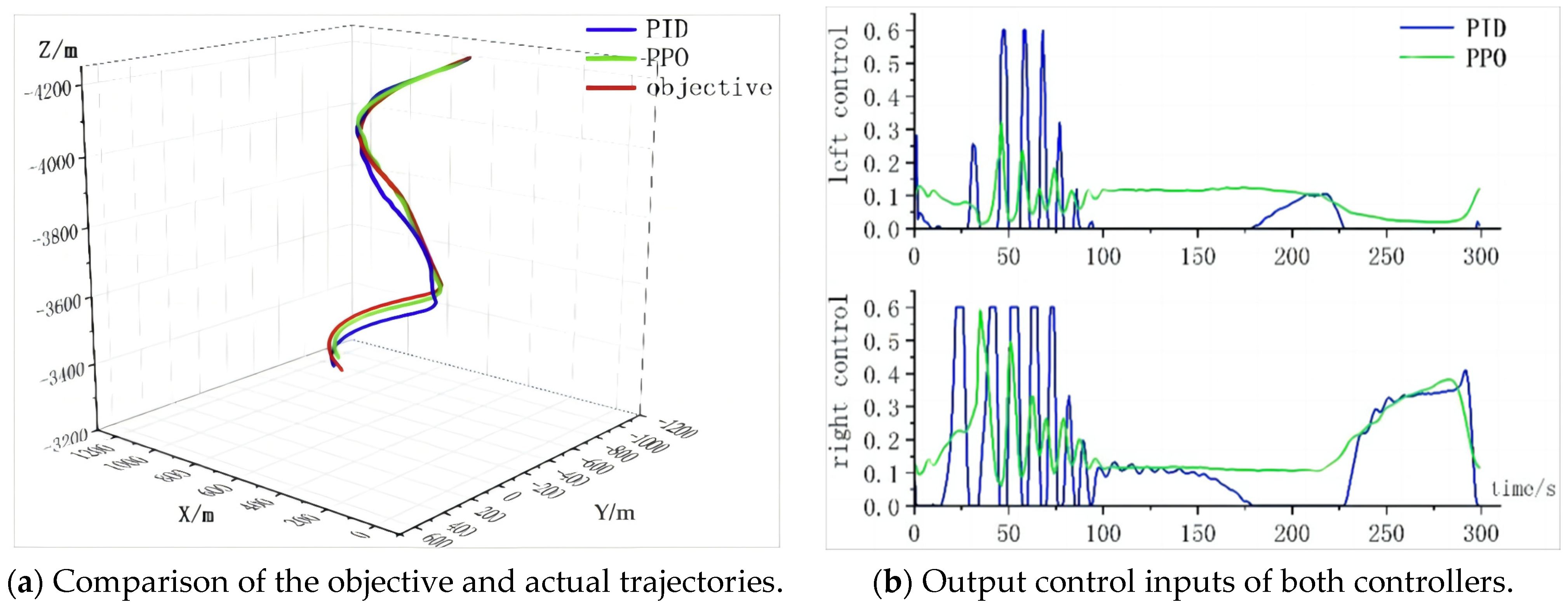
During the parafoil single-flight test simulation experiment, one objective trajectory is chosen stochastically from the test collection. Figure 13a illustrates the comparison between the 3D objective trajectory and the actual trajectory obtained using the PID and PPO parafoil motion controllers. The comparison results indicate that the actual flight trajectory achieved by the PPO parafoil motion controller is superior to that of the PID parafoil motion controller. Figure 13b displays the control quantities generated by the two controllers during the trajectory-tracking process. It can be observed from the graph that the control quantities produced by the PPO controller are smoother. Additionally, at any given moment, the PID controller can only generate one control quantity (left or right control quantity) while the other control quantity remains at 0. However, the PPO controller can simultaneously output both left and right control quantities as needed. Table 1 shows that the control precision of the PPO controller is 4 times that of the PID controller in a single flight.
(2)
Multiple Flights
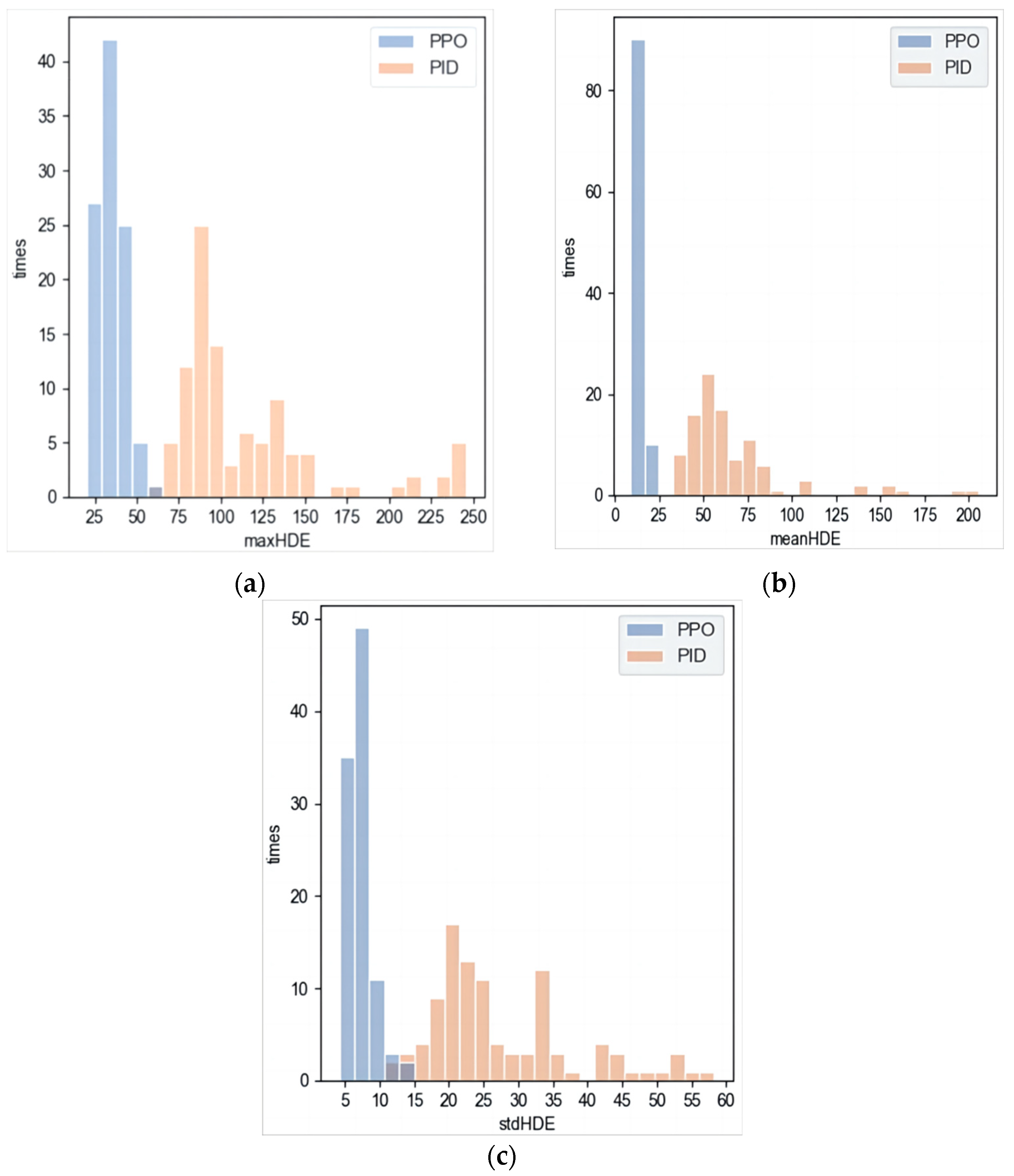
During the parafoil multiple-flight test simulation experiments, all of the 100 random objective trajectories were employed. Figure 14 shows the performance index distributions of the PID and PPO controllers over 100 flights. It can be concluded that the max_maxHDE of PID is mainly distributed between 75 and 250 m, while the max_maxHDE of PPO is mostly distributed between 20 and 57 m; the mean_meanHDE of PID and PPO are, respectively, concentrated in the range of 30 and 210 m, and 10 and 25 m; the mean_stdHDE of PID is centralized in the range of 10 and 60 m, and the mean_stdHDE of PPO is centralized in the range of 4 and 15 m. Table 2 shows that the control precision of the PPO controller is 4 times that of the PID controller over 100 flights.

5.3.3. Influence of Environmental Conditions on the Parafoil Motion Controller

The trained parafoil motion controller is susceptible to environmental conditions. This section discusses the influence of payload weight, observation noise, and wind speed on the parafoil motion controller. The test collection of parafoil objective trajectories utilized here is the same as the one used in Section 5.3.2.
(1)
Influence of Payload Weight on the Parafoil Motion Controller
Table 3 summarizes the max_maxHDE, mean_meanHDE, and mean_stdHDE of the PID controller and PPO controller during a multiple-flight test with different payload weights. The standard payload weight in Table 3 is the one utilized in Section 5.3.2.
It can be seen in Table 3 that the impact on the performance of the parafoil motion controller due to payload weight is very slight. Furthermore, the PPO parafoil motion controller is still superior to the PID one in the case of different payload weights.
(2)
Influence of Observation Noise on the Parafoil Motion Controller
Considering that there is an error caused by the observation noise between the observed state and the real state of the parafoil, this study presents test simulation experiments to demonstrate the effect of observation noise on the performance of the parafoil motion controller. The test simulation experiment is performed with the standard payload weight employed in Section 5.3.2.
The x, y, and z observed coordinates of the parafoil are used as the input information of the parafoil motion controller. The observation noise can be added to the observed coordinates of the parafoil. According to the different settings of the observation noise, the test simulation experiment is divided into two groups.
The first type of noise, the observation noise (Gaussian random noise with mean = 0 and standard deviation = SD), is independent of time. In each step of the parafoil motion-control training, three values of the observation noise are, respectively, added into the x, y, and z coordinates of the parafoil.
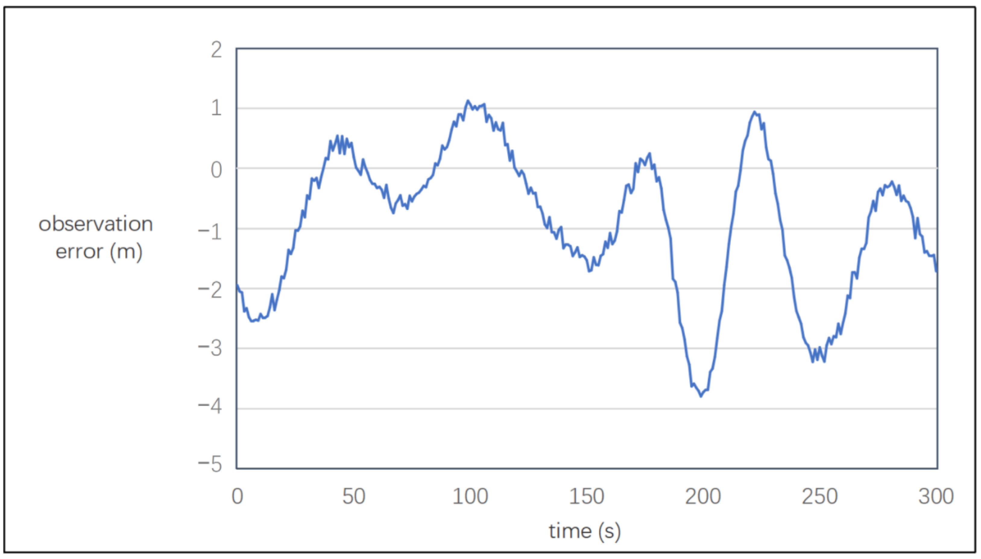
The second type of noise, the observation noise (here, the first type of noises are first sampled with an interval of 20 points or 20 s; the internal noises are interpolated with these existing noises and then add another Gaussian random noise with mean = 0 and standard deviation = 0.1 × SD), is time-dependent. In the 300-step parafoil motion-control training, the curve of observation noise (with SD = 2) added into the z coordinate of the parafoil versus time is shown in Figure 15.
The experimental data of the parafoil motion controllers based on PID and PPO In time of multiple flights with the first and second types of noise are summarized in Table 4. It can be seen in Table 4 that the parafoil motion controller based on PID is more susceptible to the first type of noise, and the performance indexes of the PID parafoil motion controller become worse as the standard deviation (SD) increases. The parafoil motion controller based on PPO is more sensitive to the second type of noise, and the performance indexes of the PPO parafoil motion controller get poorer as the standard deviation (SD) increases. In summary, the overall performance of the PPO parafoil motion controller is preferable to that of the PID controller.
(3)
Influence of Wind Speed on the Parafoil Motion Controller
Considering that wind is the most import influence factor of parafoil flights, this study presents test simulation experiments to demonstrate the effect of wind on the performance of parafoil motion controllers. The test simulation experiment is performed with the standard payload weight employed in Section 5.3.2 and assumes that there is no observation noise. During the test simulation experiments, 100 random objective trajectories under different wind speeds’ influence (without wind, 0–2 m/s wind speed, 2–4 m/s wind speed, and 4–7 m/s wind speed) have been employed.
It can be seen in Table 5 that the performance of both controllers deteriorates with the increase in wind speed, but the PPO controller always outperforms the PID controller.

6. Real Flight Evaluation

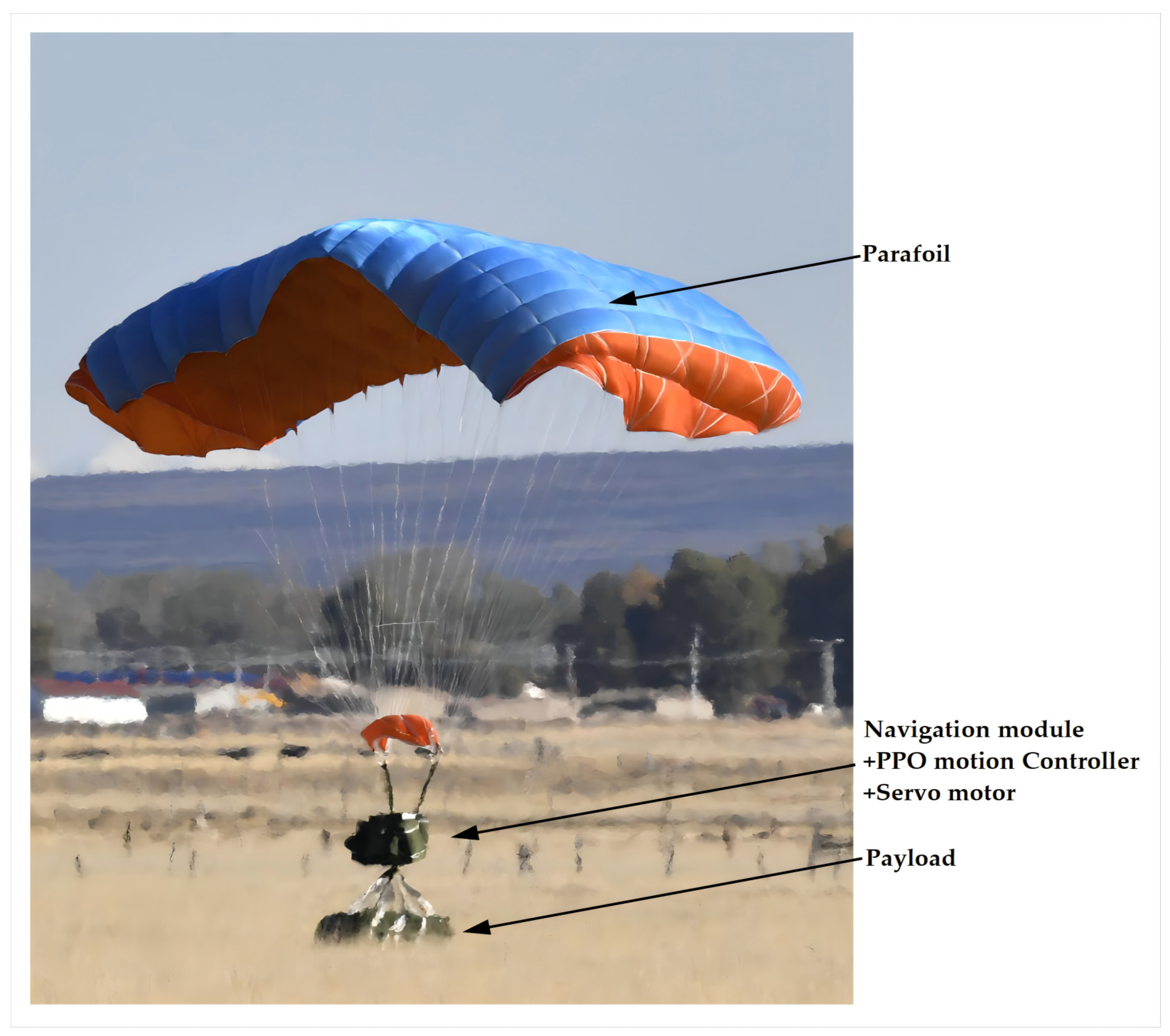
To evaluate the performance of the PPO parafoil motion controller trained by the proposed simulation training system, a real flight test of the parafoil system was conducted. The parafoil system, including the parafoil, navigation system, and control system, is shown in Figure 16. The information on the flight test is listed in Table 6. The size and weight of the parafoil system in Table 6 are the same as the one used in the simulation verification in Section 5.
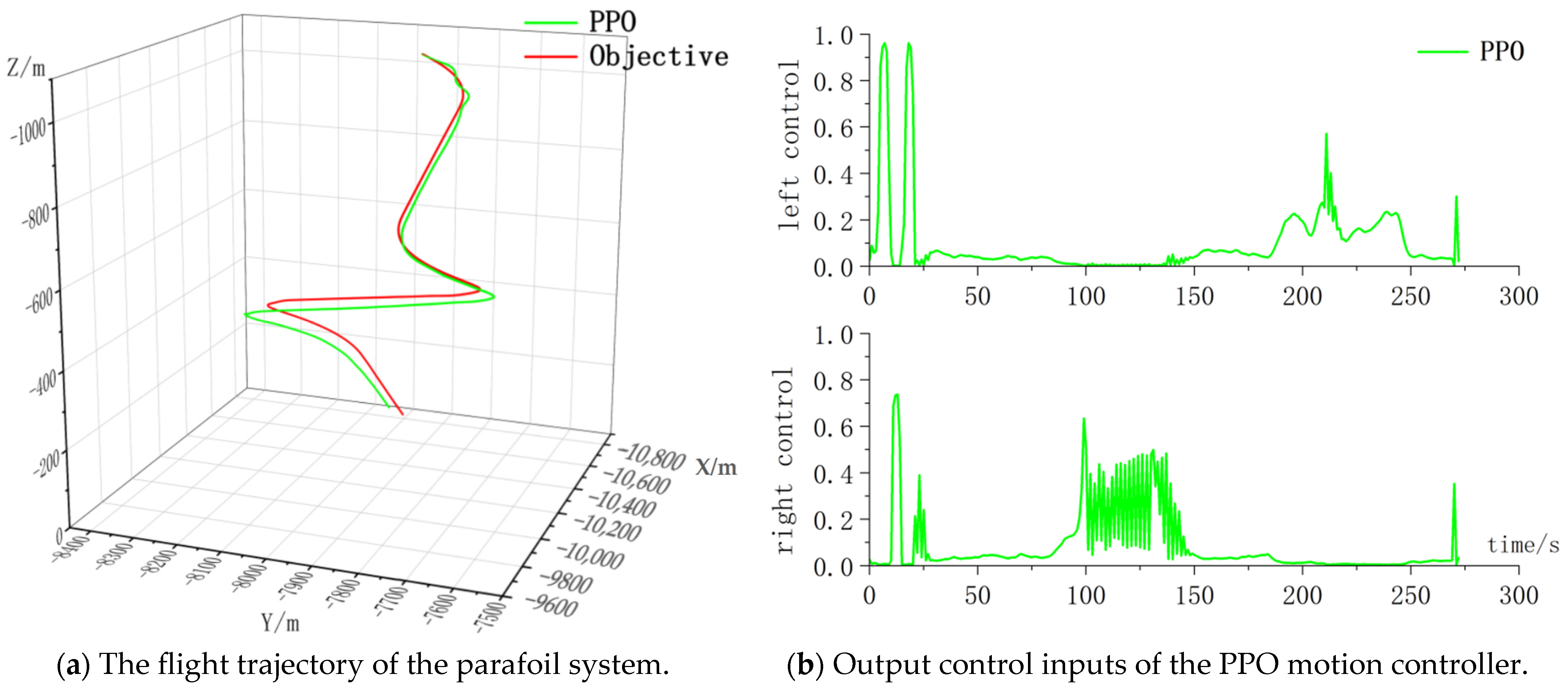
Figure 17a shows the flight-trajectory comparison in the height range from 100 to 1000 m between the real flight based on the PPO motion controller and the objective trajectory. The left and right control quantities of the PPO motion controller are depicted in Figure 17b. In addition, the trajectory-tracking performance details of the real flight are listed in Table 7.
Although the variations in the two control quantities in real flight are greater than those in the simulation scenario in the comparison of Figure 13 and Figure 17, it is apparent that the performance indexes of the PPO controller in Table 7 are not worse than the ones in Table 5. In addition, compared with the high cost of the real flight, the parafoil simulation system can perform a comprehensive evaluation of the PPO motion controller proposed in this study at a very low cost.

7. Conclusions

In order to improve the control precision of the parafoil system, this study presents an actor–critic RL simulation training system to train the parafoil motion controller and make it achieve high adaptability to specific parafoil models and environmental conditions. The simulations and comparisons in Section 5 between the classic PID and PPO motion controllers prove the superior control effect of the parafoil motion controller trained by the simulation training system introduced in this study. The PPO controller can perform parafoil motion control with a mean tracking position precision of less than 14 m in the ideal case (with a standard payload weight, no observation noise, and no wind) and a mean tracking position precision of less than 80 m in bad cases (with a non-standard payload weight, observation noise, and wind, respectively) in this study’s experiments. Additionally, the test results of the real flight experiment are comparable to the simulation results.

Author Contributions

Conceptualization, X.H. and J.L.; methodology, R.X. and Q.L.; software, J.W.; validation, G.Y. and J.Z.; resources, J.L.; writing—original draft preparation, J.Z. All authors have read and agreed to the published version of the manuscript.

Funding

This research was funded by the Major State Basic Research Development Programme of China, grant number 2018YFE0206500, and the Ministry of Education G China Mobile Scientific Research Fund, grant number MCM2020—JG1.

Data Availability Statement

All data used to support the findings of this study are included within the article.

Conflicts of Interest

The authors declare no conflicts of interest. The funding sponsors had no role in the design of the study; in the collection, analyses, or interpretation of data; in the writing of the manuscript, and in the decision to publish the results.

Appendix A

Observation state: The observation state information used in this study is presented in Table A1.
Table A1. Observation state.
State SymbolState NameMinimum ValueMaximum Value
EASVelocity angle deviation−180°180°
EFRDescent rate deviation−22
AtProspective angle (8-dimensional)−90°90°
Dp2tTarget point distance0.0 (m)200.0 (m)
Ap2tTarget point angle−180°180°
ClActual left control quantity01
CrActual right control quantity01
AwpAngle between wind and target trajectory direction−180°180°
ωhHorizontal modulus of the wind0 m/s10 m/s
ωvVertical component of a wind−1 m/s1 m/s
The calculation methods for each component of the observation state are as follows:
Given the coordinates of the parafoil at the current time as P = P x , P y , P z and the coordinates at the previous time as P = P x , P y , P z . Then, the horizontal velocity direction angle A s p and the descent rate F R p of the parafoil at the current time can be calculated as follows:
A sp = tan 1 P y p y P x p x
FR p = P z P z P x P x , P y P y
First, it can be assumed that the current time coordinates of the parafoil’s reference target point (located on the target trajectory) are denoted as D o = ( D x o , D y o , D z o ) , and the coordinates of the reference target point at the next time step are expressed as D p = ( D x p , D y p , D z p ) . Then, the target horizontal velocity direction angle A s t and the target descent rate F R t of the parafoil at the current time can be calculated as follows:
A st = tan 1 D y p D y o D x p D x o
FR t = D z p D z o D x p D x o , D y p D y o
Then, we can obtain the velocity angle deviation E A S and the descent rate deviation E F R :
EAS = ASpASt
EFR = FRpFRt
Giving the coordinates of three reference target points as D o = D x o , D y o , D z o , D a = D x a , D y a , D z a and D b = D x b , D y b , D z b , the prospective angle At can be defined as follows:
A t = mod   A 1 A 0 , 180,180
where the function mod converts the input value (A1A0) to a value in the range of [−180, 180], and
A 0 = tan 1 D y a D y 0 D x a D x 0
A 1 = tan 1 D y b D y a D x b D x a
In this study, the reference point is the point in front of the parafoil on the target trajectory. The prospective distance parameter is set as V = 100 m (forward from parafoil in z direction), and the target trajectory within this interval is divided into 9 vector line segments (10 points in total) at equal intervals. The prospective angle values are calculated for each adjacent two vector segments, and a total of eight prospective angle features are obtained. Therefore, the actual A t used in the experiment is an 8-dimensional vector.
The target point distance D p 2 t and target point angle A p 2 t between the current coordinates of the parafoil P and the coordinates of the target point D o can be defined as follows:
D p 2 t = D 0 P
A P 2 t = mod tan 1 D y 0 P y D x 0 P x A s t , 180,180
The actual left (right) control quantity C l ( C r ) represents the value of the parafoil actually performed at the current moment, which is directly obtained from the parafoil simulation environment.
If the wind vector is W = ( W x , W y , W z ) , θ w is the direction angle of the wind field calculated by W, and θ p is the true course angle, then the angle between wind and the target trajectory direction can be expressed as
A wp = mod θ w θ p , 180,180
The horizontal modulus of the wind is
w h = W x 2 + W y 2
The vertical component of a wind is ωv = WZ.
To normalize all states based on their maximum and minimum values, the normalization formula used is as follows:
S = S S m i n S m a x S m i n

Appendix B

Action: The actions are the desired lengths of the left and right control ropes pulled down by the actuator simulation module based on the controller’s output. For easier training, this study normalizes the actions by dividing them with the maximum allowed pull-down length. The actuator simulation module can perform the inverse operation before executing the action. Therefore, the actions of the parafoil are expressed as Al and Ar, which are in the range of [0, 1].

Appendix C

Reward: In this study, we adopted the sparse reward approach, which only provides rewards upon reaching the terminal state. Let T be the maximum number of steps in an episode (default value of 100). Te represents the actual number of executed steps, satisfying TeT. Di denotes the distance between the parafoil and the reference point (the point on the target trajectory with the same parafoil z-coordinate) after each step. D0 represents the maximum distance (a default value of 200 m) between the parafoil and the reference point. If DiD0, the parafoil enters a dead state, and the flight is terminated. The calculation formula is as follows:
r = 1 T i = 1 T e D i + T T e × 1.2 × D e

Appendix D

Objective Trajectory: To generate objective trajectories, the parafoil will start from an altitude of 9000 m and follow a random action sequence P = A i , t i i = 1,2 , , N until reaching ground. This process will be repeated to generate 1000 objective trajectories for training purposes and 100 objective trajectories for testing purposes.
The random action sequence P = A i , t i i = 1,2 , , N is generated using the single-sided pull-down random action sequence generation method. Each item A i , t i in the random action sequence is generated as follows:
l o r = r a n d o m 1 , 1
α i = c l i p r a n d o m r 0 1 r 0 , 1 , 0.1 × l m a x
A i = α i 0 , 0 α i , l o r 0 l o r > 0
t i = r a n d o m T 1 , T 2
In the given context:
l o r ” represents the flag indicating the type of control. Values less than or equal to 0 denote a left control, while values greater than 0 indicate a right control. The probability of left and right control is evenly distributed at 50% each.
l m a x ” belongs to the interval [0, 1] and represents the maximum absolute magnitude of the control quantity. This means that the generated control quantities will not exceed this value.
r0” belongs to the interval [0, 1) and represents the probability of the control quantities being 0. The probability falling within the range (0, l m a x ] is equal to 1 − r0.
[ T 1 , T 2 ] ” represents the range of possible duration for each action.
By incorporating these parameters, the random action sequence is generated according to the specified probabilities and constraints, ensuring a variety of pull-down actions with different durations. By setting the four parameters (lmax, r0, T1, T2) in the algorithm, it is possible to generate a diverse set of random action sequences with different characteristics. This, in turn, can lead to the creation of target trajectory sets with varying features. The values of the four parameters in this study are as follows: lmax = 0.3, r0 = 0.33, T1 = 10, T2 = 120.

Appendix E

Design of the PPO Network: The PPO network consists of an actor network and a critic network, with the network structure closely related to the parafoil trajectory-tracking problem. The number of nodes in the network input layer is 17, which is determined by the dimension of the observation state. The number of nodes in the actor network output layer is two, which is determined by the dimension of the action. The output of the critic network is a scalar value, so the output layer has one node. The actor network has two hidden layers, with 32 and 32 nodes, respectively, and the critic network has three hidden layers, with 64, 32, and 16 nodes, respectively. The overall network structure (the number of hidden layers and the number of nodes per layer) was designed with reference to network structure designs for similar problems, such as the intelligent control of unmanned devices based on reinforcement learning, and then adjusted. We found that 2–4 hidden layers and 16–64 nodes for each layer could obtain good results, and we chose the best setting. The activation functions used were the sigmoid and tanh functions, which are widely applied in neural networks.

References

  1. Tan, P.L.; Luo, S.Z.; Sun, Q.L. Control strategy of power parafoil system based on coupling compensation. Trans. Beijing Inst. Technol. 2019, 39, 378–383. [Google Scholar]
  2. Zhu, H.; Sun, Q.; Wu, W.N.; Sun, M.; Chen, Z. Accurate modeling and control for parawing unmanned aerial vehicle. Acta Aeronaut. Astronaut. Sin. 2019, 40, 79–91. [Google Scholar]
  3. Li, Y.; Zhao, M.; Yao, M.; Chen, Q.; Guo, R.P.; Sun, T.; Jiang, T.; Zhao, Z.H. 6-DOF modeling and 3D trajectory tracking control of a powered parafoil system. IEEE Access. 2020, 8, 151087–151105. [Google Scholar] [CrossRef]
  4. Zhao, L.G.; He, W.L.; Lv, F.K. Model-free adaptive control for parafoil systems based on the iterative feedback tuning method. IEEE Access. 2021, 9, 35900–35914. [Google Scholar] [CrossRef]
  5. Zhao, L.G.; He, W.L.; Lv, F.K.; Wang, X.G. Trajectory tracking control for parafoil systems based on the model-free adaptive control. IEEE Access. 2020, 8, 152620–152636. [Google Scholar] [CrossRef]
  6. Tao, J. Research on Modeling and Homing Control of Parafoil Systems in Complex Environments. Ph.D. Thesis, Nankai University, Tianjin, China, 2017. [Google Scholar]
  7. Tao, J.; Sun, Q.L.; Chen, Z.Q.; He, Y.P. LADAR-based trajectory tracking control for a parafoil system. J. Harbin Eng. Univ. 2018, 39, 510–516. [Google Scholar]
  8. Sun, Q.L.; Chen, S.; Sun, H.; Chen, Z.Q.; Sun, M.W.; Tan, P.L. Trajectory tracking control of powered parafoil under complex disturbances. J. Harbin Eng. Univiron. 2019, 40, 1319–1326. [Google Scholar]
  9. Jia, H.C.; Sun, Q.L.; Chen, Z.Q. Application of Single Neuron LADRC in Trajectory Tracking Control of Parafoil System. In Proceedings of the 2018 Chinese Intelligent Systems Conference, Wenzhou, China, 6 October 2018; pp. 33–42. [Google Scholar]
  10. Jagannath, J.; Jagannath, A.; Furman, S.; Gwin, T. Deep Learning and Reinforcement Learning for Autonomous Unmanned Aerial Systems: Roadmap for Theory to Deployment, 1st ed.; Springer: Berlin, Germany, 2020. [Google Scholar]
  11. Polosky, N.; Jagannath, J.; Connor, D.O.; Saarinen, H.; Foulke, S. Artificial neural network with electroencephalogram sensors for brainwave interpretation: Brain-observer-indicator development challenges. In Proceedings of the 13th International Conference and Expo on Emerging Technologies for a Smart World, Location of Conference, Stony Brook, NY, USA, 7–8 November 2017; Saarinen, H., Ed.; 8 November 2017. [Google Scholar]
  12. Jagannath, A.; Jagannath, J.; Drozd, A. Artificial intelligence-based cognitive cross-layer decision engine for next-generation space mission. In Proceedings of the 2019 IEEE Cognitive Communications for Aerospace Applications Workshop, Cleveland, OH, USA, 25–26 June 2019. [Google Scholar]
  13. Jagannath, A.; Jagannath, J.; Drozd, A. Neural network for signal intelligence: Theory and practice. In Machine Learning for Future Wireless Communications, 1st ed.; Luo, F., Ed.; John Wiley & Sons Ltd.: Hoboken, NJ, USA, 2020; pp. 243–264. [Google Scholar]
  14. Chen, Y.; Dong, Q.; Shang, X.Z.; Wu, Z.Y.; Wang, J.Y. Multi-UAV autonomous path planning in reconnaissance missions considering incomplete information: A reinforcement learning method. Drones 2023, 7, 10. [Google Scholar] [CrossRef]
  15. Jiang, N.; Jin, S.; Zhang, C.S. Hierarchical automatic curriculum learning: Converting a sparse reward navigation task into dense reward. Neurocomputing 2019, 360, 265–278. [Google Scholar] [CrossRef]
  16. Yang, W.Y.; Bai, C.J.; Cai, C.; Zhao, Y.N.; Liu, P. Survey on sparse reward in deep reinforcement learning. Comput. Sci. 2019, 47, 182–191. [Google Scholar]
  17. Zhao, X.R.; Yang, R.N.; Zhong, L.S.; Hou, Z.W. Multi-UAV path planning and following based on multi-agent reinforcement learning. Drones 2024, 8, 18. [Google Scholar] [CrossRef]
  18. Guo, Y.M.; Yan, J.G.; Xing, X.J.; Wu, C.H.; Chen, X.R. Modeling and analysis of deformed parafoil recovery system. J. Northwest. Polytech. Univ. 2020, 38, 952–958. [Google Scholar] [CrossRef]
  19. Gao, F. Study on Homing Strategy for Parafoil System under Wind Field. Master Thesis, University of Defense Technology, Changsha, China, 2019. [Google Scholar]
  20. Liu, S.Q.; Bai, J.Q. Analysis of flight energy variation of small solar UAVs using dynamic soaring technology. J. Northwest. Polytech. Univ. 2020, 38, 48–57. [Google Scholar] [CrossRef]
  21. Yu, J.; Sun, H.; Sun, J.Q. Improved twin delayed deep deterministic policy gradient algorithm based real-time trajectory planning for parafoil under complicated constrains. Appl. Sci. Basel. 2022, 12, 8189. [Google Scholar] [CrossRef]
  22. Xing, X.J.; Gong, Q.C.; Guan, X.Q.; Han, Y.C.; Feng, L.; Guo, Y.M. Online trajectory planning for parafoil first-stage booster system in complex wind field. J. Aerosp. Eng. 2023, 36, 04023027. [Google Scholar] [CrossRef]
  23. Sutton, R.S.; Barto, A.G. Reinforcement Learning: An Introduction, 2nd ed.; The MIT Press: Cambridge, MA, USA, 2018; pp. 1–398. [Google Scholar]
  24. Schulman, J. Research on Modeling and Homing Control of Parafoil Systems in Complex Environments Proximal Policy Optimization Algorithms. Ph.D. Thesis, Cornell University, Ithaca, NY, USA, 2017. [Google Scholar]
  25. Lynch, K.M.; Park, F.G. Modern Robotics-Mechanics, Planning, and Control, 1st ed.; Cambridge University Press: New York, NY, USA, 2017; pp. 1–642. [Google Scholar]
  26. Prakash, O.; Ananthkrishnan, N. Modeling and simulation of 9-DOF parafoil-payload system flight dynamics. In Proceedings of the AIAA Atmospheric Flight Mechanics Conference and Exhibit, Keystone, CO, USA, 21–24 August 2006. [Google Scholar]
  27. Ochi, Y. Modeling and simulation of flight dynamics of a relative-roll-type parafoil. In Proceedings of the AIAA Scitech 2020 Forum, Orlando, FL, USA, 6–10 January 2020. [Google Scholar]
  28. Prakash, O.; Kumar, A. NDI based heading tracking of hybrid-airship for payload delivery. In Proceedings of the AIAA Scitech 2022 Forum, San Diego, CA, USA, 3–7 January 2022. [Google Scholar]
  29. Prakash, O. Modeling and simulation of turning flight maneuver of winged airship-payload system using 9-DOF multibody model. In Proceedings of the AIAA Scitech 2023 Forum, National Harbor, MD & Online, USA, 23–27 January 2023. [Google Scholar]
  30. Bian, K. Trajectory. Master Thesis, University of Defense Technology, Changsha, China, 2020. [Google Scholar]
  31. Hao, R.; Meng, B. Research on gust direction and suggestion for flight operation. J. Civ. Aviat. Inst. China 2021, 5, 89–92. [Google Scholar]
  32. Haarnoja, T.; Zhou, A.; Abbeel, P.; Levine, S. Soft actor-critic: Off-policy maximum entropy deep reinforcement learning with a stochastic actor. In Proceedings of the 35th International Conference on Machine Learning, PMLR, Stockholm, Sweden, 10–15 July 2018. [Google Scholar]
  33. Haarnoja, T.; Zhou, A.; Hartikainen, K.; Tucker, G.; Ha, S.; Tan, J.; Kumar, V.; Zhu, H.; Gupta, A.; Abbeel, P.; et al. Soft actor-critic algorithms and applications. arXiv 2018, arXiv:1812.05905. [Google Scholar]
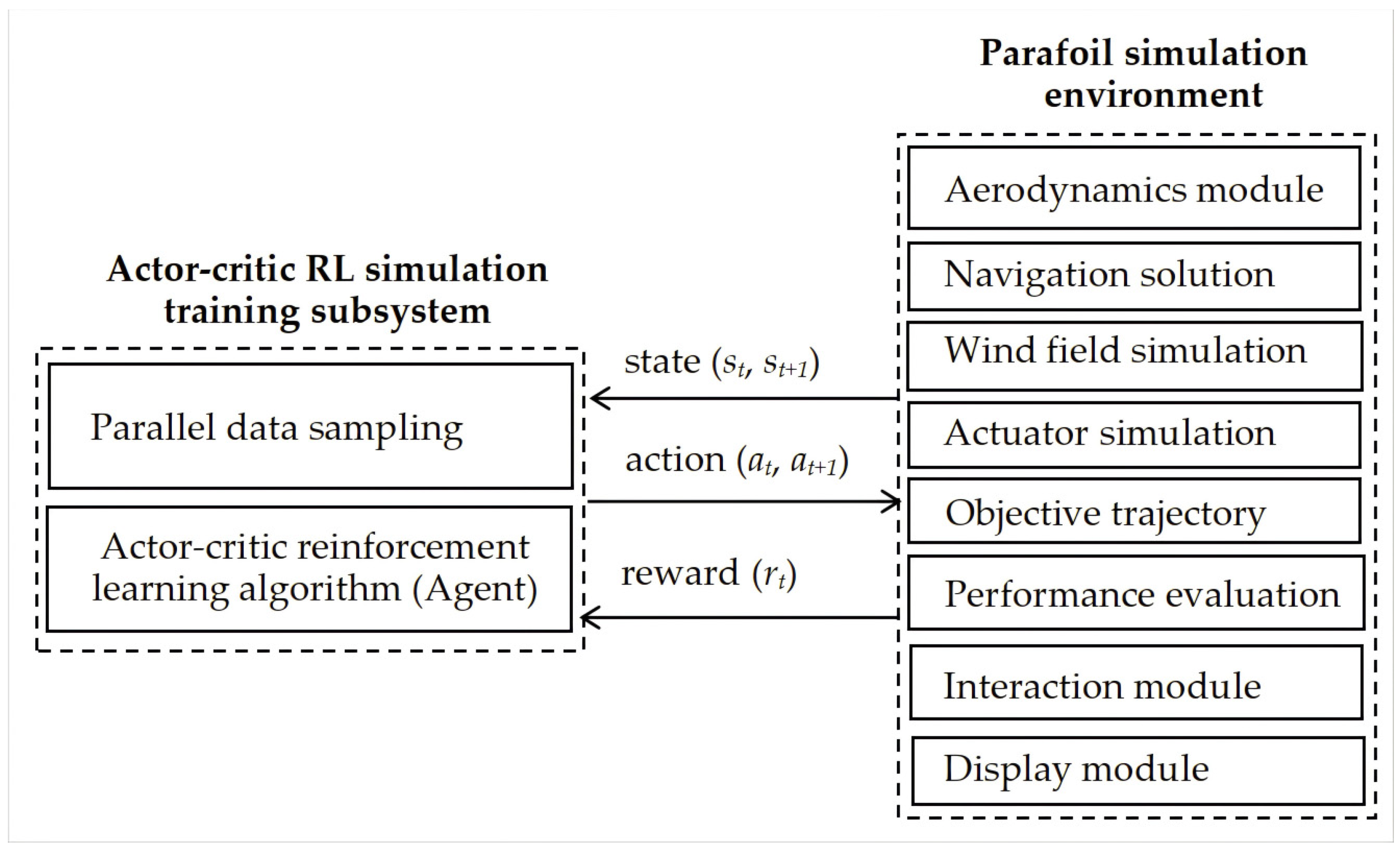
Figure 1. Framework of the introduced parafoil motion-control-simulation training system.
Actuators 13 00280 g001
Figure 2. Relationship among all the modules of the parafoil simulation environment.
Actuators 13 00280 g002
Figure 3. Basic working principle of the motor constrained by the trapezoidal velocity profile.
Actuators 13 00280 g003
Figure 4. Schematic diagram of the parafoil–payload system.
Actuators 13 00280 g004
Figure 5. Navigation solution diagram of the parafoil simulation environment.
Actuators 13 00280 g005
Figure 6. Flowchart of the parafoil motion-control-simulation training.
Actuators 13 00280 g006
Figure 7. Parallel sampling structure with one GPU and multiple CPUs.
Actuators 13 00280 g007
Figure 8. Common structure of the actor–critic algorithm.
Actuators 13 00280 g008
Figure 9. PPO network structure. (a) is an actor network, and (b) is a critic network.
Actuators 13 00280 g009
Figure 10. Procedure of the parafoil motion-control-simulation training.
Actuators 13 00280 g010
Figure 11. Curves of average reward per episode in the training process with initial values of standard deviation for sampling, respectively, equal to 0.3 (red curve), 0.5 (yellow curve), and 0.75 (blue curve).
Actuators 13 00280 g011
Figure 12. Curves of average reward per episode in the training process with initial values of the learning rate magnitude order severally equal to 1.0 × 10⁻³ (blue curve), 1.0 × 10⁻⁴ (green curve), 1.0 × 10⁻⁵ (yellow curve), and 1.0 × 10⁻⁶ (red curve).
Actuators 13 00280 g012
Figure 13. Performance comparison of the PID and PPO controllers in a single flight. (a) is a comparison of the objective trajectory and the actual trajectory, and (b) is the output control inputs of both controllers.
Actuators 13 00280 g013
Figure 14. Performance histograms of the PID and PPO controllers over 100 flights. (a) is a statistical result of the “max_maxHDE”, (b) is a statistical result of the “mean_meanHDE”, and (c) is a statistical result of the “mean_stdHDE”.
Actuators 13 00280 g014
Figure 15. Curve of observation noise added into the z coordinate of the parafoil versus time.
Actuators 13 00280 g015
Figure 16. Experimental parafoil system with navigation module and the proposed PPO motion controller.
Actuators 13 00280 g016
Figure 17. A real flight based on PPO motion controller. (a) is a comparison of the actual trajectory with the objective trajectory, and (b) is a practical result of the two control quantities of the PPO motion controller.
Actuators 13 00280 g017
Table 1. Performance indexes of the PID and PPO controllers in a single flight.
Parafoil Motion ControllermaxHDE (m)meanHDE (m)stdHDE (m)
PID236.5767.5825.41
PPO49.1516.236.59
Table 2. Performance indexes of the PID and PPO controllers over 100 flights.
Parafoil Motion Controllermax_maxHDE (m)mean_meanHDE (m)mean_stdHDE (m)
PID245.7866.9129.04
PPO57.0813.887.48
Table 3. Performance indexes of the PID and PPO controllers over 100 flights with different payload weights.
max_maxHDE (m)mean_meanHDE (m)mean_stdHDE (m)
0.5 × Standard payload weight
PID234.6764.7225.46
PPO77.6412.547.79
Standard payload weight
PID245.7866.9129.04
PPO57.0813.887.48
2 × Standard payload weight
PID224.8584.0232.55
PPO73.3521.4610.85
Table 4. Performance indexes of the PID and PPO controllers in N = 100 flights with different observation noise.
max_maxHDE (m)mean_meanHDE (m)mean_stdHDE (m)
Without observation noise
PID245.7866.9129.04
PPO57.0813.887.48
The first type of noise (SD = 1)
PID422.54147.6473.32
PPO108.0827.2113.53
The first type of noise (SD = 2)
PID1027.10240.71125.75
PPO188.6157.5029.45
The second type of noise (SD = 1)
PID326.7493.6745.60
PPO154.7132.1317.79
The second type of noise (SD = 2)
PID330.9995.3845.05
PPO388.2178.9445.73
Table 5. Performance indexes of the PID and PPO controllers in N = 100 flights with different wind speeds.
max_maxHDE (m)mean_meanHDE (m)mean_stdHDE (m)
Without wind
PID245.7866.9129.04
PPO57.0813.887.48
0–2 m/s
PID333.5594.6446.07
PPO257.0831.2122.38
2–4 m/s
PID461.10107.7155.04
PPO310.6231.5221.59
4–7 m/s
PID909.99176.39109.23
PPO412.2250.9439.61
Table 6. Physical parameters of the parafoil and experiment conditions.
ParametersValues
Wing span and wing chord/m7.5, 3.75
Maximum takeoff weight/kg200
Empty weight/kg25
Payload/kg135
Flight time/sec272
Wind directionSoutheast
Wind speed/(m/s)1.98–3.89
WeatherCloudless
Temperature/°C20
Table 7. Performance indexes of the PPO controller in a real flight.
maxHDE (m)meanHDE (m)stdHDE (m)
PPO111.6152.0536.21
Disclaimer/Publisher’s Note: The statements, opinions and data contained in all publications are solely those of the individual author(s) and contributor(s) and not of MDPI and/or the editor(s). MDPI and/or the editor(s) disclaim responsibility for any injury to people or property resulting from any ideas, methods, instructions or products referred to in the content.