
Investigation on the Reduced-Order Model for the Hydrofoil of the Blended-Wing-Body Underwater Glider Flow Control with Steady-Stream Suction and Jets Based on the POD Method


Abstract
1. Introduction
2. Model and Method
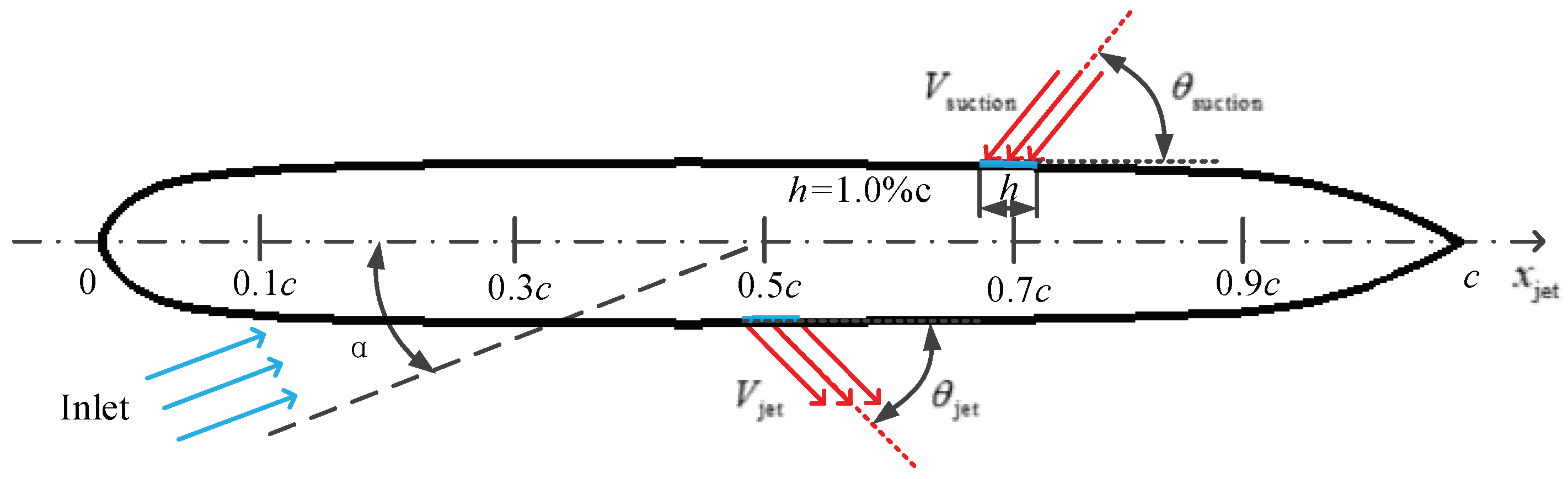
2.1. Physical Model
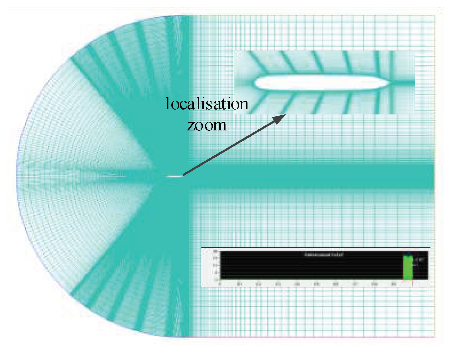
2.2. Numerical Sampling Method
2.3. POD Method
3. Discussion and Analysis of Results
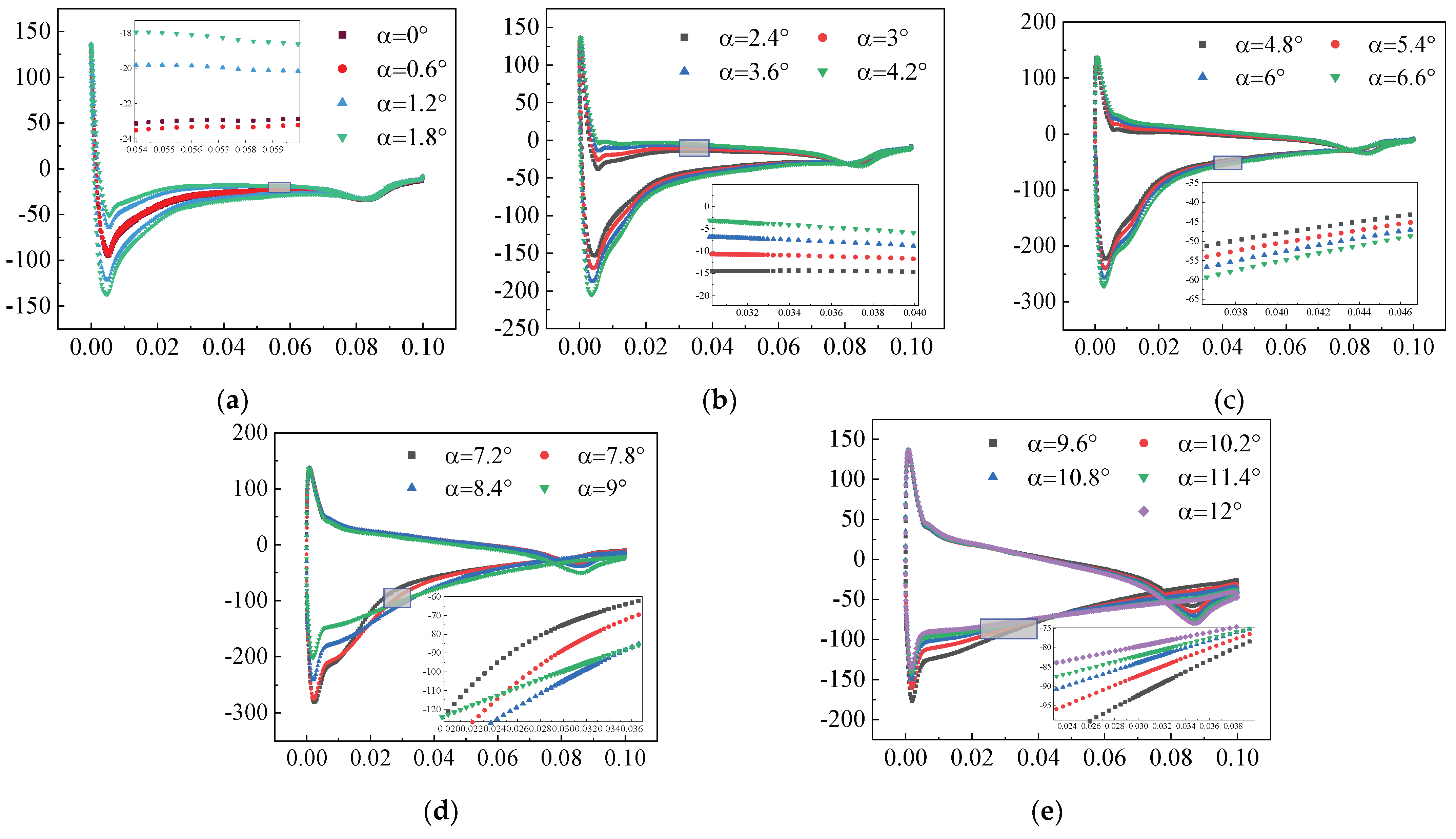
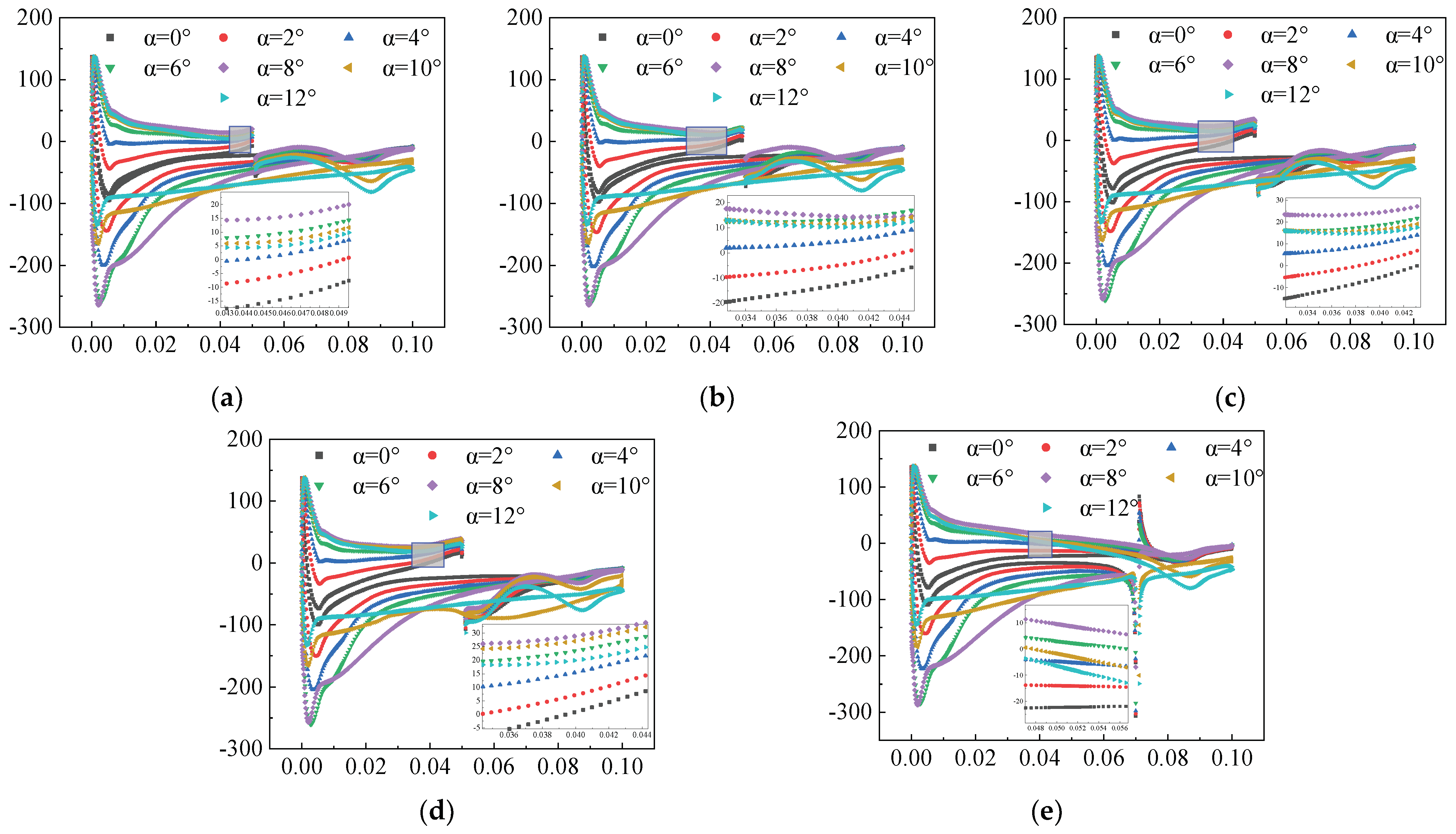
3.1. Flow Field Information Sampling
3.1.1. Flow Field without AFC
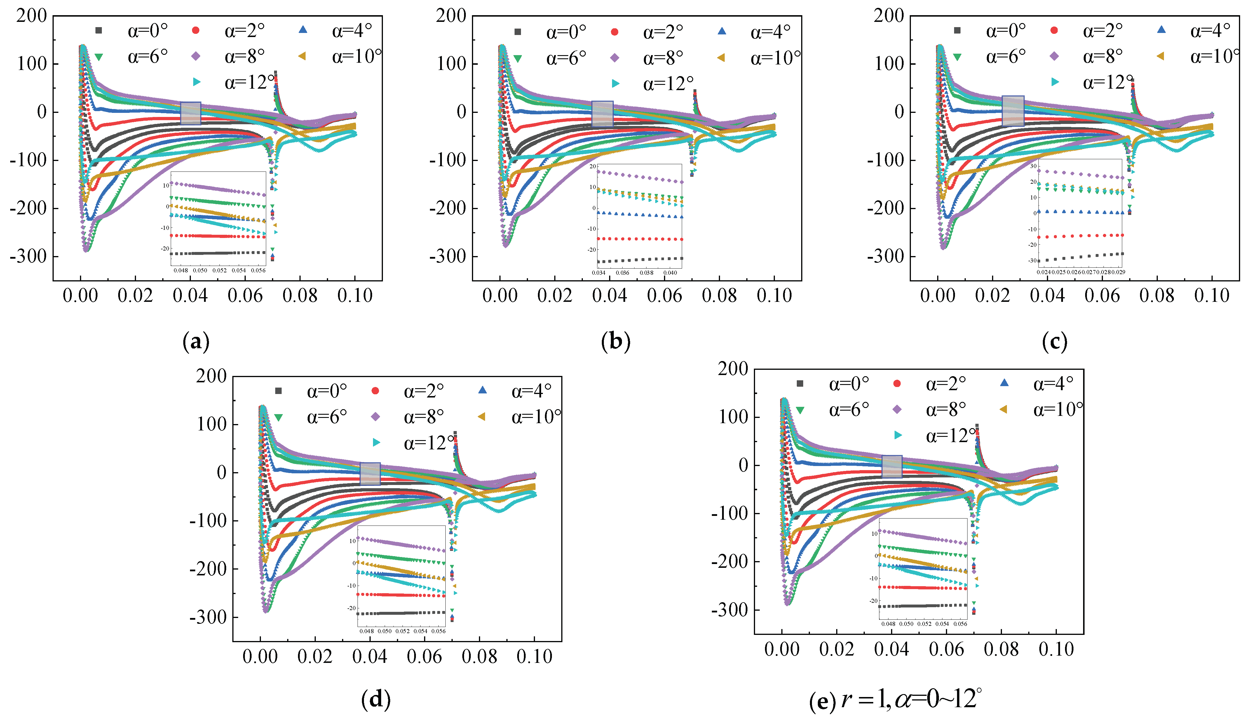
3.1.2. Constant Suction Control Flow Field
3.1.3. Constant Jet Control Flow Field
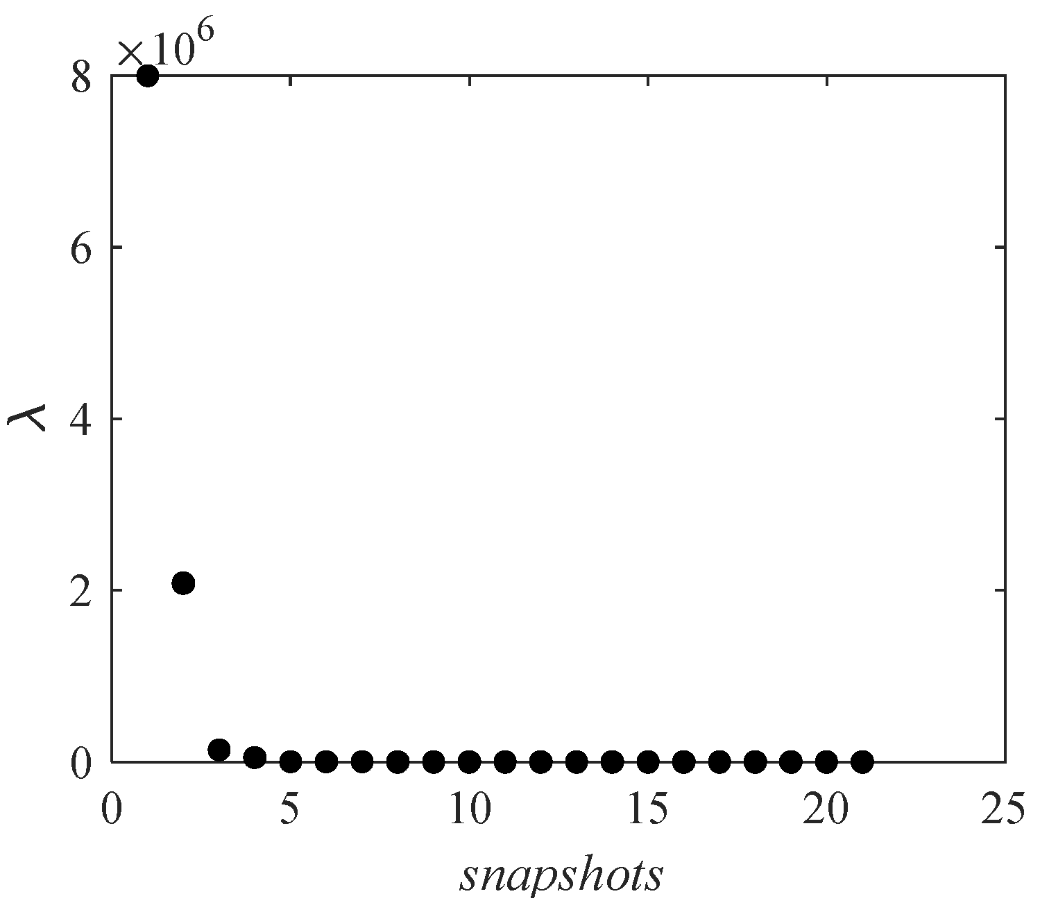
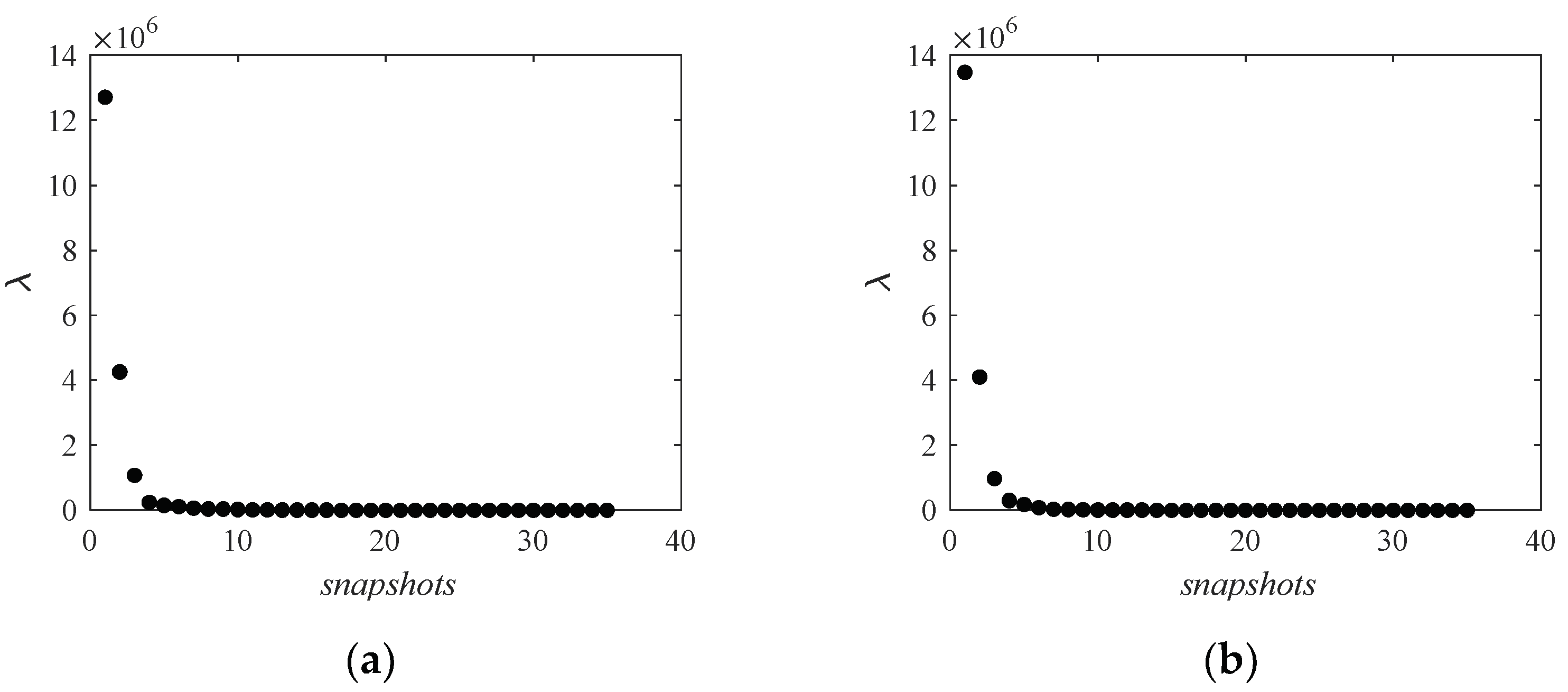
3.2. Reconstruction of Flow Field Based on the POD Method
3.2.1. Flow Field without AFC
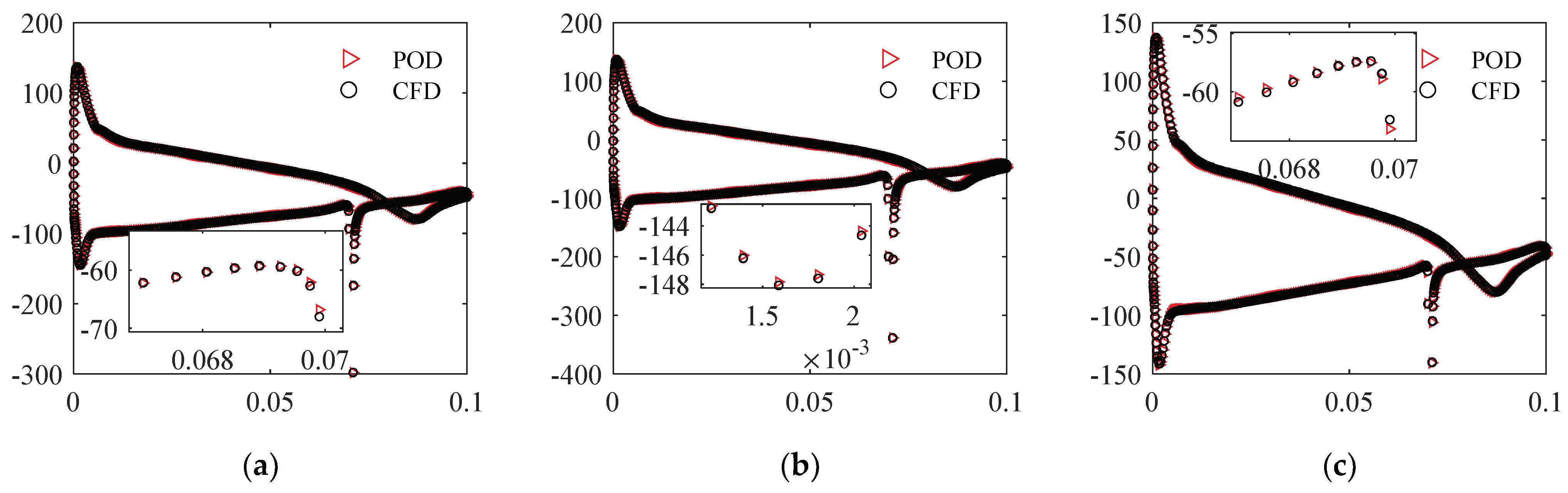
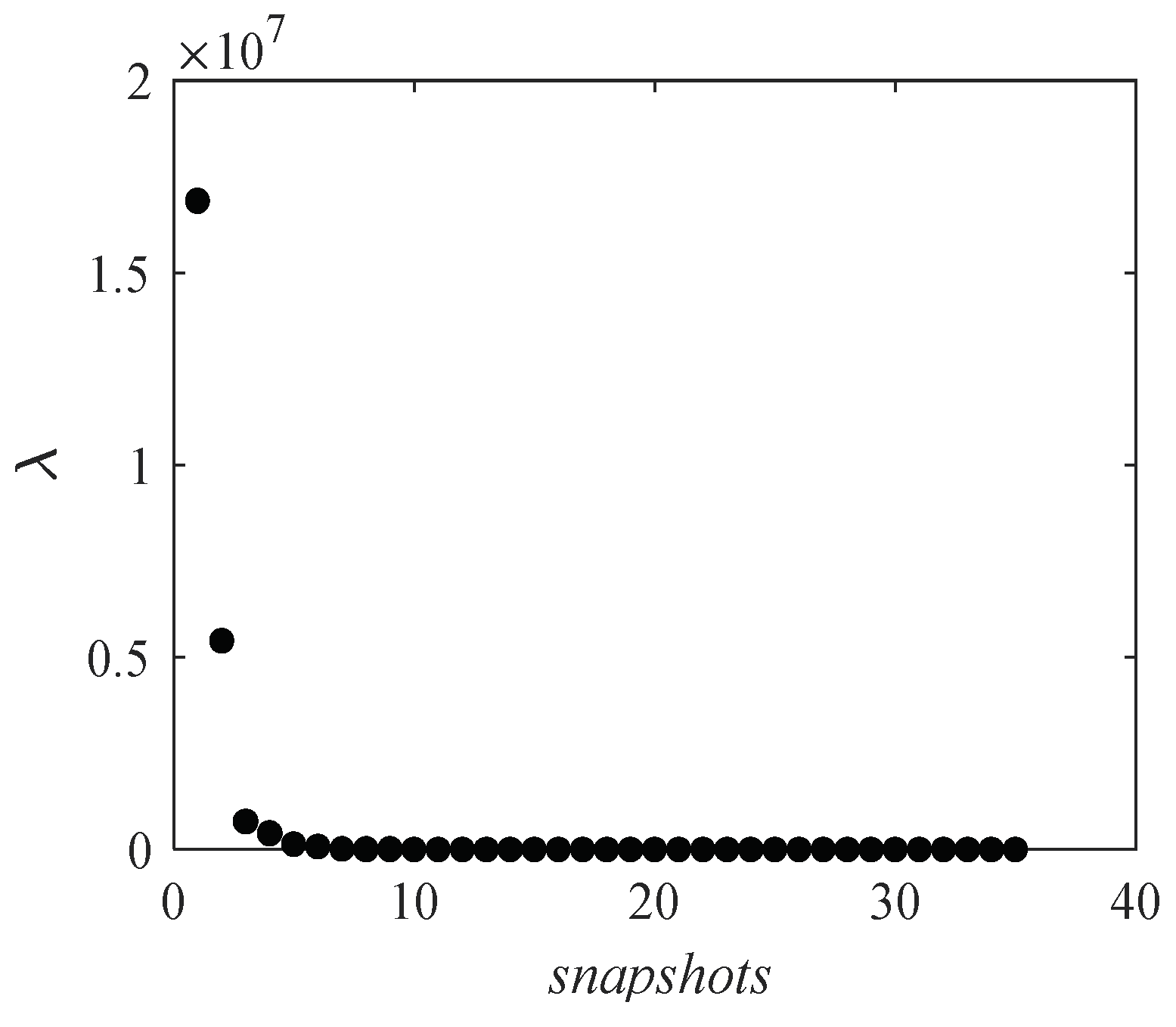
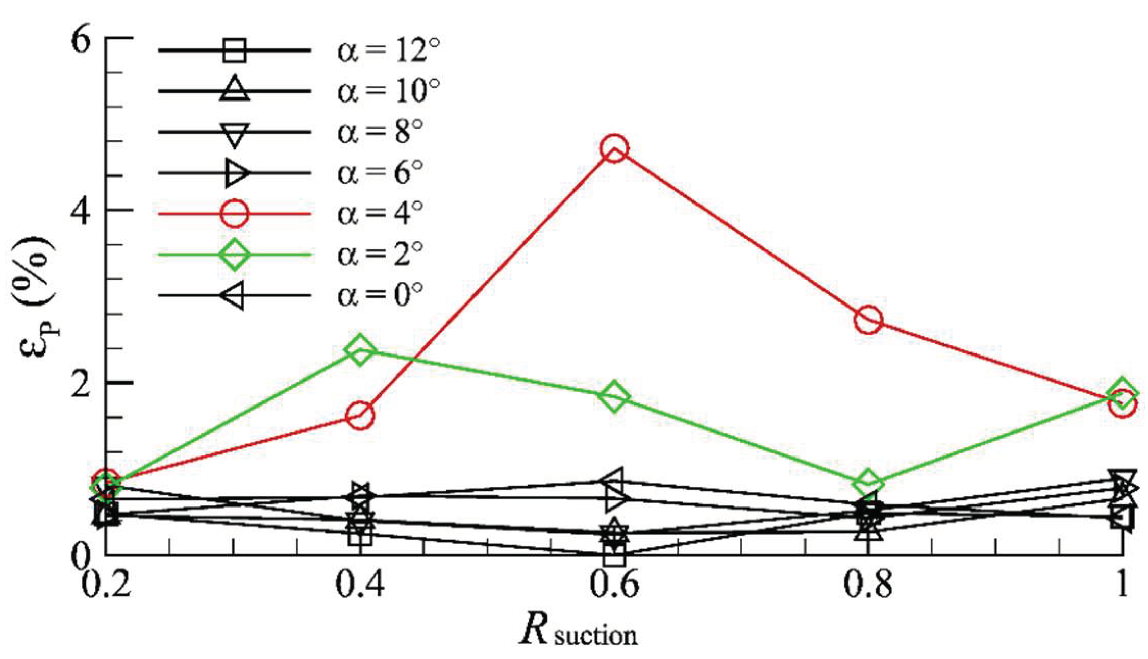
3.2.2. Constant Suction Control Flow Field
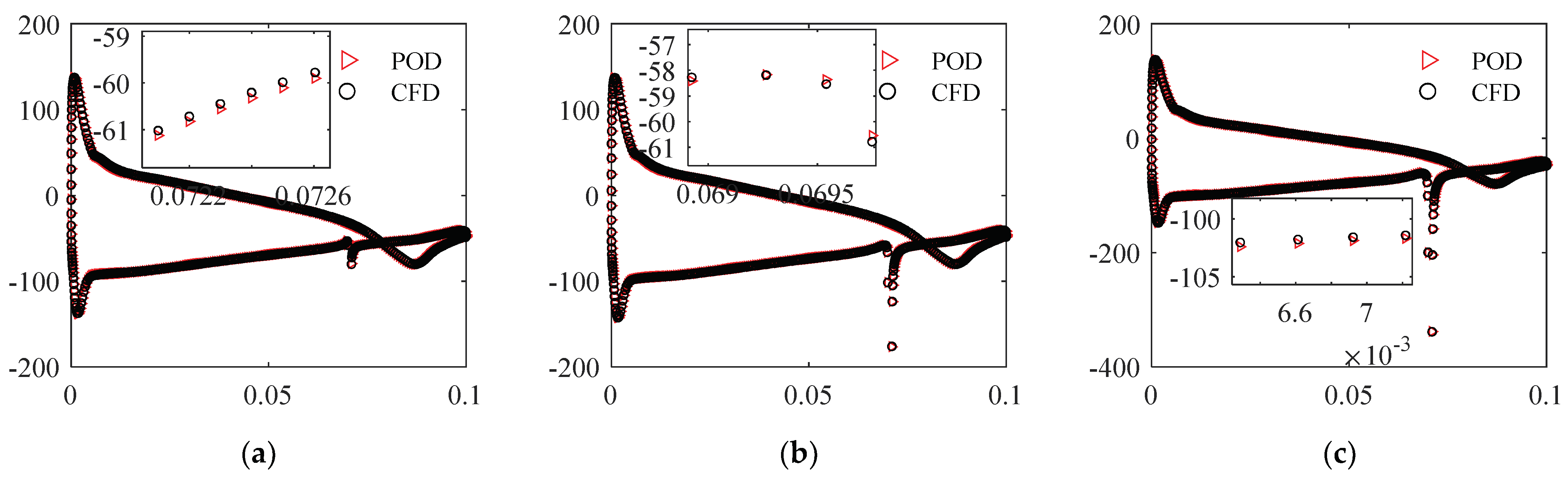
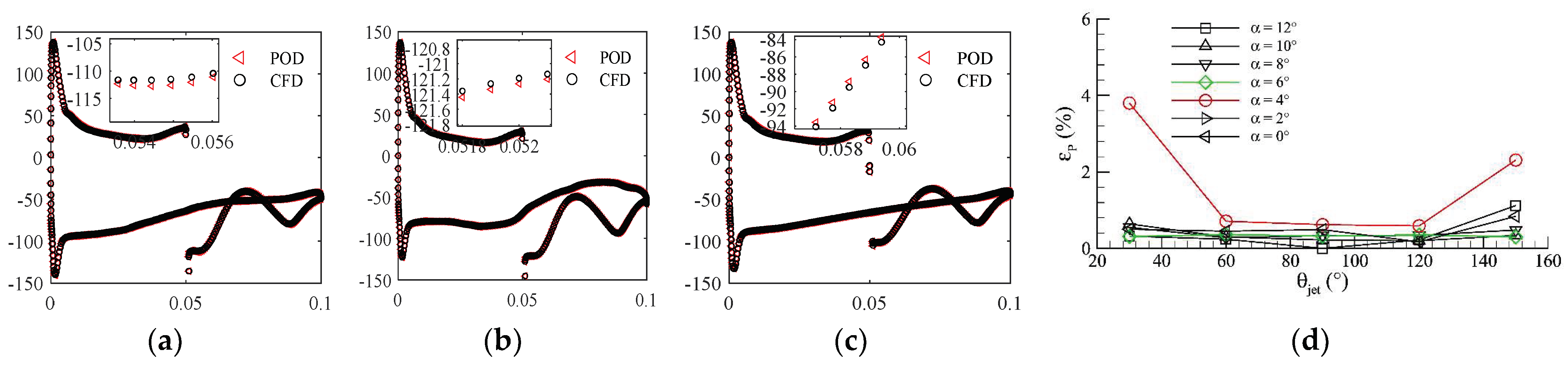
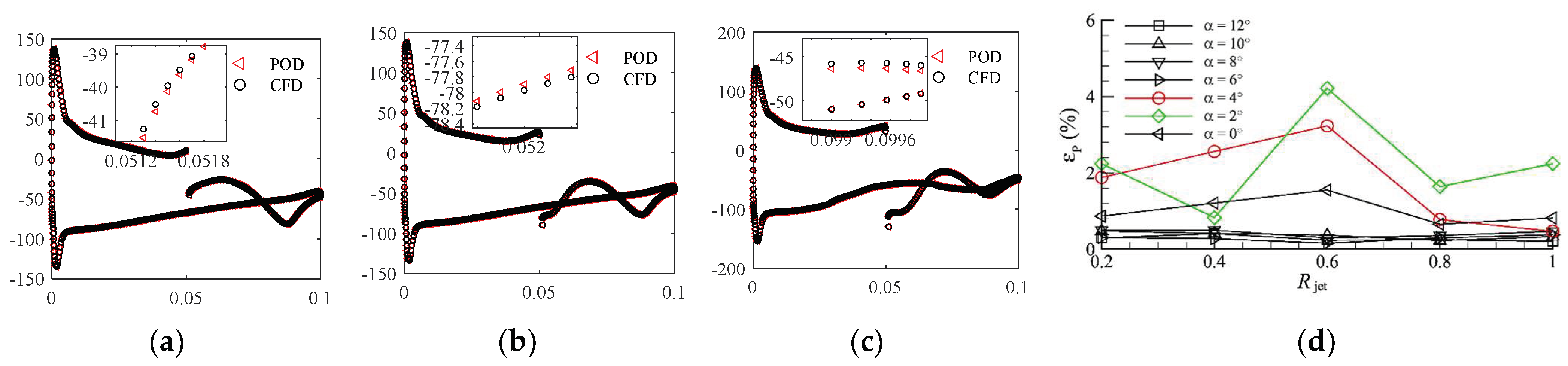
3.2.3. Constant Jet Control Flow Field
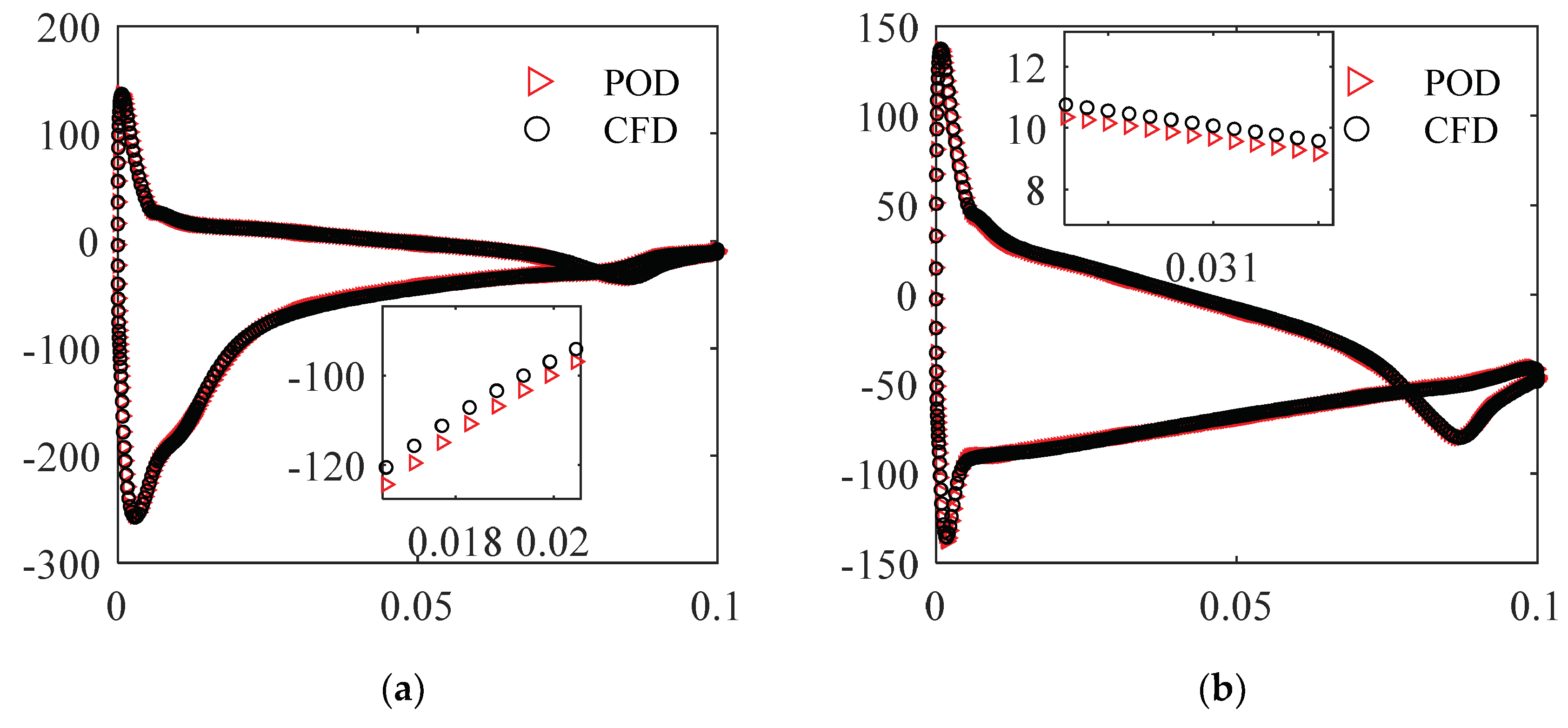
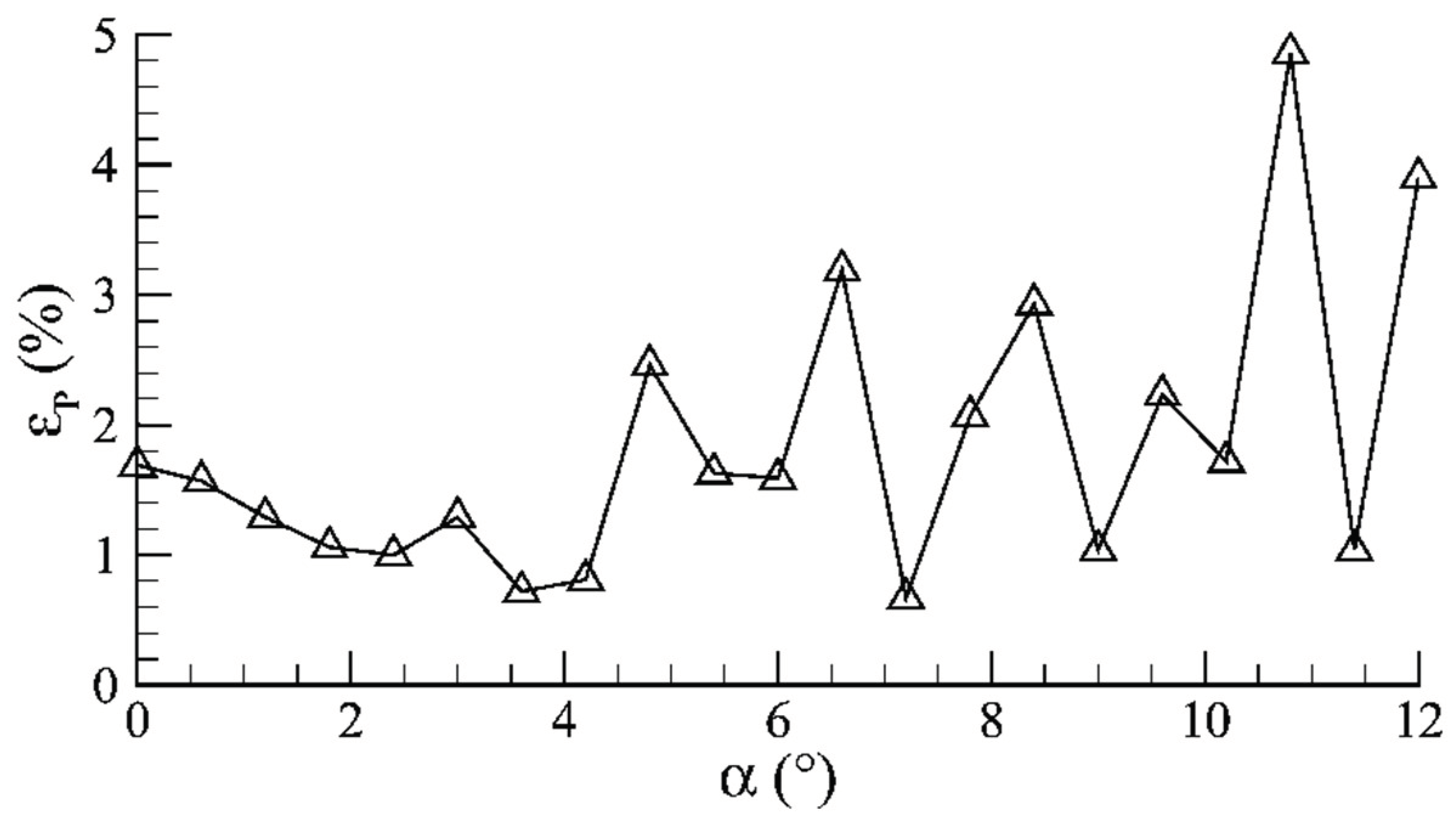
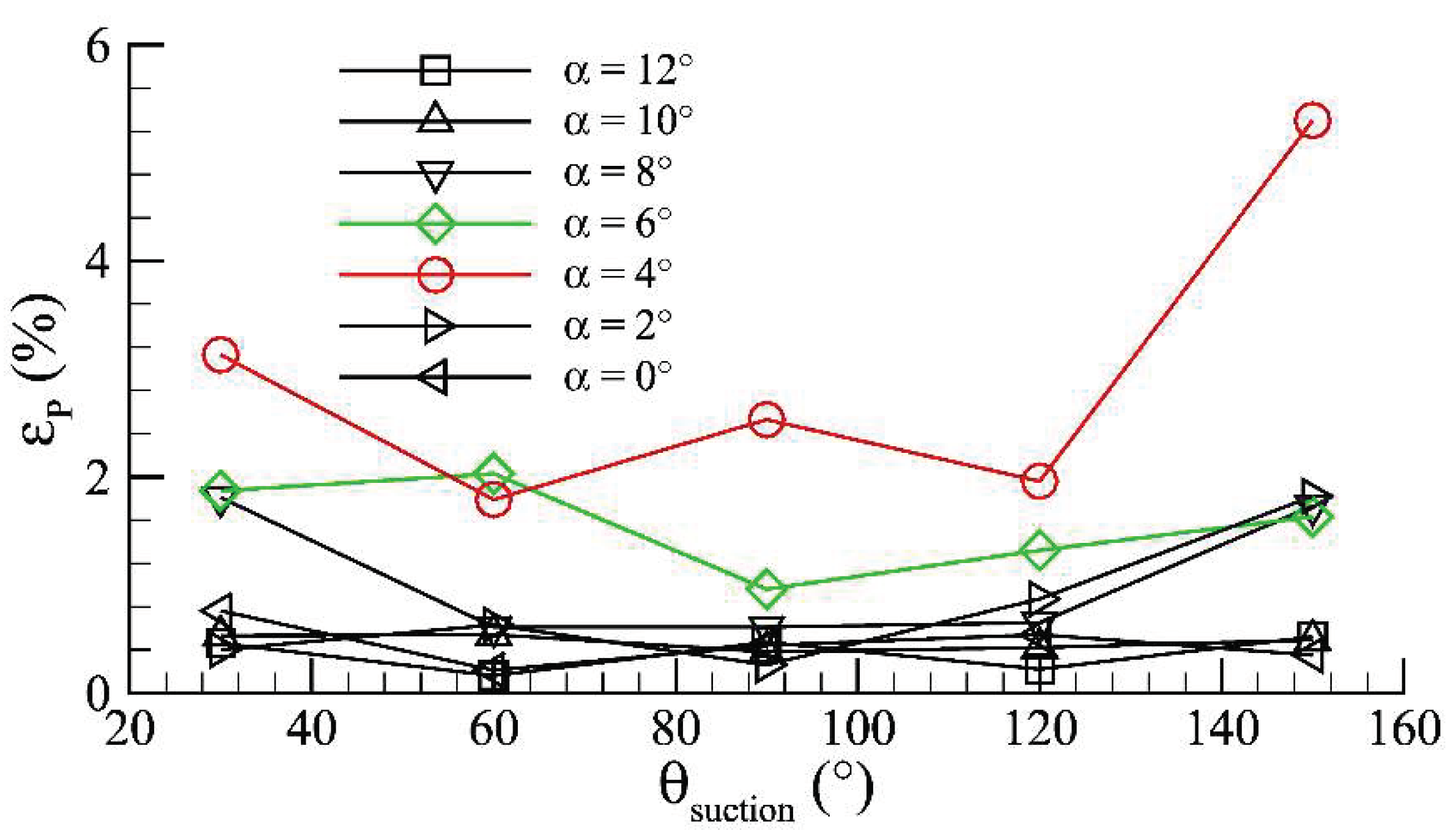
3.3. POD-ROM Flow Field Prediction
4. Conclusions
Author Contributions
Funding
Data Availability Statement
Conflicts of Interest
References
- Sun, C.Y.; Song, B.W.; Wang, P. Shape design and hydrodynamic characteristics analysis of the blended-wing-body underwater glider. J. Ship Sci. Technol. 2016, 38, 78–83. (In Chinese) [Google Scholar]
- Du, X.X.; Zhang, L.Y. Numerical study on the steady suction active flow control of hydrofoil in the profile of the blended-wing-body underwater glider. J. Northwestern Polytech. Univ. 2021, 39, 801–809. (In Chinese) [Google Scholar] [CrossRef]
- Zhang, X.L.; Du, X.X.; Ran, X.Z. Numerical Research on Active Flow Control with Synthetic Jet for Wing Section of Underwater Blended-wing-body Glider. Shipbuild. China 2022, 63, 95–106. (In Chinese) [Google Scholar]
- Ren, F.; Wang, C.; Tang, H. Bluff body uses deep-reinforcement-learning trained active flow control to achieve hydrodynamic stealth. Phys. Fluids 2021, 33, 093602. [Google Scholar] [CrossRef]
- Lu, T.; Hu, H.; Song, J.; Ren, F. Lattice Boltzmann modeling of backward-facing step flow controlled by a synthetic jet. J. Hydrodyn. 2023, 35, 757–769. [Google Scholar] [CrossRef]
- Dong, H.; Geng, X.; Shi, Z.; Cheng, K.; Cui, Y.D.; Khoo, B.C. On evolution of flow structures induced by nanosecond pulse discharge inside a plasma synthetic jet actuator. Jpn. J. Appl. Phys. 2019, 58, 028002. [Google Scholar] [CrossRef]
- Zhang, H.; Feng, Y. Review of Flow Control by Lorentz Force. Aerodyn. Res. Exp. 2023, 1, 20–29. (In Chinese) [Google Scholar]
- Du, X.X.; Liu, X.; Song, D. Coupled physics analysis of blended-wing-body underwater glider equipped with electromagnetic active flow control. Ocean. Eng. 2023, 278, 114402. [Google Scholar] [CrossRef]
- Zhang, L.; Gao, S.Q.; Zhao, J.X.; Tang, C.; Xie, H.L. Numerical simulation of influence of steady inhalation on aerodynamic performance of wind turbine. Acta Energiae Solaris Sin. 2018, 39, 2155–2162. (In Chinese) [Google Scholar]
- Zhou, X.B.; Zhou, S.; Hou, A.P.; Zheng, X.Q. Numerical Investigation on Controlling Separated Cascade Flows by Using Jets. Acta Aeronaut. Et Astronaut. Sinica 2007, 28S, 7–13. (In Chinese) [Google Scholar]
- Wang, B.X.; Yang, Z.G.; Zhu, H.; Li, Y.L. Drag Reducition by Active Control with Steady Blowing/Suction Methods. J. Tongji Univ. (Nat. Sci.) 2017, 45, 1383–1389. (In Chinese) [Google Scholar]
- Du, X.; Liu, X.; Song, Y. Analysis of the Steady-Stream Active Flow Control for the Blended-Winged-Body Underwater Glider. J. Mar. Sci. Eng. 2023, 11, 1344. [Google Scholar] [CrossRef]
- Chen, G.; Li, Y.M. Advances and prospects of the reduced-order for unsteady flow and its application. Adv. Mech. 2011, 41, 686–701. [Google Scholar]
- Ren, F.; Gao, C.Q.; Tang, H. Machine learning for flow control: Applications and development trends. Acta Aeronaut. Et Astronaut. Sin. 2021, 42, 524686. [Google Scholar]
- Ye, K.; Wu, J.; Ye, Z.Y.; Qu, Z. Analysis Circular Cylinder Flow Using Dynamic Mode and Proper Orthogonal Decomposition. J. Northwestern Polytech. Univ. 2017, 35, 599–607. [Google Scholar]
- Lumley, J.L. Rational approach to relations between motions of differing scales in turbulent flows. Phys. Fluids 1967, 10, 1405–1408. [Google Scholar] [CrossRef]
- Kidambi, K.B.; Mackunis, W.; Jayaprakash, A.K. Limit Cycle Oscillation Suppression Using a Closed-Loop Nonlinear Active Flow Control Technique. In Proceedings of the 59th IEEE Conference on Decision and Control (CDC), Jeju, Republic of Korea, 14–18 December 2020. [Google Scholar] [CrossRef]
- Axia, W.; Yichen, M.; Wenjing, Y. The proper orthogonal decomposition method for the Navier-Stokes equations. Acad. J. Xi'an Jiaotong Univ. 2008, 20, 141–148. [Google Scholar]
- Min, G.; Jiang, N. Data-driven identification and pressure fields prediction for parallel twin cylinders based on POD and DMD method. Phys. Fluids 2024, 36, 023614. [Google Scholar] [CrossRef]
- Sun, F.J.; Zhu, D.H.; Zhang, D.M. Reduced-order model for fluid-structure coupled calculation of wind turbine blades. J. Vib. Shock. 2021, 40, 175–181+215. (In Chinese) [Google Scholar]
- Wang, Y.G.; Li, Z.N.; Gong, B.; Li, Q.S. Reconstruction & prediction of wind pressure on heliostat. Acta Aerodyn. Sin. 2009, 27, 586–591. (In Chinese) [Google Scholar]
- Kang, W.; Zhang, J.Z.; Li, K.L. Nonlinear Galerkin Method for Dimension Reduction Using Proper Orthogonal Decomposition. J. Xi'an Jiaotong Univ. 2011, 45, 58–62+67. (In Chinese) [Google Scholar]
- Anderson, J.D.; Wendt, J. Computational Fluid Dymanics; McGraw-Hill Companies: New, York, NY, USA, 1995. [Google Scholar]
- Menter, F.R. Two-equation eddy-viscosity turbulence models for engineering applications. AIAA J. 1994, 32, 1598–1605. [Google Scholar] [CrossRef]
- Eiximeno, B.; Miró, A.; Rodríguez, I.; Lehmkuhl, O. Toward the Usage of Deep Learning Surrogate Models in Ground Vehicle Aerodynamics. Mathematics 2024, 12, 998. [Google Scholar] [CrossRef]
- Lu, K.; Jin, Y.; Chen, Y.; Yang, Y.; Hou, L.; Zhang, Z.; Li, Z.; Fu, C. Review for order reduction based on proper orthogonal decomposition and outlooks of applications in mechanical systems. Mech. Syst. Signal Process. 2019, 123, 264–297. [Google Scholar] [CrossRef]


| Mesh Number | Lift Coefficient | ||
|---|---|---|---|
| AOA = 2° | AOA = 6° | AOA = 10° | |
| 76000 | 0.2683 | 0.5895 | 0.5384 |
| 105000 | 0.2639 | 0.5886 | 0.5378 |
| 135000 | 0.2612 | 0.5861 | 0.5352 |
| 164000 | 0.2612 | 0.586 | 0.535 |
| Ordinal | Eigenvalue | Cumulative Captured Energy (%) |
|---|---|---|
| 1 | 7.99 × 10⁶ | 77.82 |
| 2 | 2.08 × 10⁶ | 98.09 |
| 3 | 1.40 × 10⁵ | 99.45 |
| Ordinal | Eigenvalue | Cumulative Captured Energy (%) |
|---|---|---|
| 1 | 1.73 × 10⁷ | 70.73 |
| 2 | 6.09 × 10⁶ | 95.58 |
| 3 | 4.76 × 10⁵ | 97.52 |
| … | … | … |
| 11 | 8.84 × 10² | 99.99 |
| Ordinal | Eigenvalue | Cumulative Captured Energy (%) |
|---|---|---|
| 1 | 1.69 × 10⁷ | 71.26 |
| 2 | 5.43 × 10⁶ | 94.19 |
| 3 | 7.25 × 10⁵ | 97.52 |
| ... | … | … |
| 11 | 1.20 × 10³ | 99.99 |
| Predicted Working Conditions | Working Condition Parameters | Computational Time(s) | ||
|---|---|---|---|---|
| POD | CFD | |||
| Flow field without AFC | α = 7.5° | 0.1 | 675 | 1.78 |
| Suction-controlled flow field | α = 3°, θ = 75° Ratio = 1.0 | 0.1 | 1516 | 4.27 |
| α = 3°, Ratio = 0.5 θ = 90° | 0.1 | 1770 | 3.42 | |
| Blowing controlled flow field | α = 3°, θ = 75° Ratio = 1.0, | 0.1 | 575 | 6.90 |
| α = 3°, Ratio = 0.5 θ = 90° | 0.1 | 445 | 1.59 | |
Disclaimer/Publisher’s Note: The statements, opinions and data contained in all publications are solely those of the individual author(s) and contributor(s) and not of MDPI and/or the editor(s). MDPI and/or the editor(s) disclaim responsibility for any injury to people or property resulting from any ideas, methods, instructions or products referred to in the content. |
© 2024 by the authors. Licensee MDPI, Basel, Switzerland. This article is an open access article distributed under the terms and conditions of the Creative Commons Attribution (CC BY) license (https://creativecommons.org/licenses/by/4.0/).
Share and Cite
Wang, H.; Du, X.; Hu, Y. Investigation on the Reduced-Order Model for the Hydrofoil of the Blended-Wing-Body Underwater Glider Flow Control with Steady-Stream Suction and Jets Based on the POD Method. Actuators 2024, 13, 194. https://doi.org/10.3390/act13060194
Wang H, Du X, Hu Y. Investigation on the Reduced-Order Model for the Hydrofoil of the Blended-Wing-Body Underwater Glider Flow Control with Steady-Stream Suction and Jets Based on the POD Method. Actuators. 2024; 13(6):194. https://doi.org/10.3390/act13060194
Chicago/Turabian StyleWang, Huan, Xiaoxu Du, and Yuli Hu. 2024. "Investigation on the Reduced-Order Model for the Hydrofoil of the Blended-Wing-Body Underwater Glider Flow Control with Steady-Stream Suction and Jets Based on the POD Method" Actuators 13, no. 6: 194. https://doi.org/10.3390/act13060194
APA StyleWang, H., Du, X., & Hu, Y. (2024). Investigation on the Reduced-Order Model for the Hydrofoil of the Blended-Wing-Body Underwater Glider Flow Control with Steady-Stream Suction and Jets Based on the POD Method. Actuators, 13(6), 194. https://doi.org/10.3390/act13060194