Abstract
This work introduces a novel sensing concept based on reaction forces for determining the position of the levitating magnet (mover) for magnetic levitation platforms (MLPs). Besides being effective in conventional magnetic bearings, the applied approach enables operation in systems where the mover is completely isolated from the actuating electromagnets (EMs) of the stator (e.g., located inside a sealed process chamber) while levitating at an extreme levitation height. To achieve active position control of the levitating mover by properly controlling the stator’s EM currents, it is necessary to employ a dynamic model of the complete MLP, including the reaction force sensor, and implement an observer that extracts the position from the force-dependent signals, given that the position is not directly tied to the measured forces. Furthermore, two possible controller implementations are discussed in detail: a basic PID controller and a more sophisticated state-space controller that can be chosen depending on the characteristics of the MLP and the accuracy of the employed sensing method. To show the effectiveness of the proposed position-sensing and control concept, a hardware demonstrator employing a 207 mm outer-diameter (characteristic dimension, CD) stator with permanent magnets, a set of electromagnets, and a commercial multi-axis force sensor is built, where a 0.36 kg mover is stably levitated at an extreme air gap of 104 mm.
Keywords:
magnetic levitation platform; load cell; force sensor; dynamic model; observer; controller 1. Introduction
In the literature, various types of magnetic levitation platforms (MLPs) have been investigated, which can be divided into two groups: (1) systems where the distance h between the stator and mover (i.e., the levitation height) is much smaller than the characteristic dimension of the system (i.e., the largest dimension CD of the system in Figure 1), and (2) systems where the levitation height is comparable to the characteristic dimension.
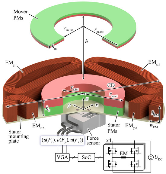
Figure 1.
Three-dimensional rendering of the magnetic levitation platform (MLP) considered in this paper, with a reaction force sensor used to determine the mover’s position. The system is actively controlled with the help of electromagnets (EMs) driven by a power converter, which is controlled by a system-on-a-chip (SoC), where an observer-based position controller (cf. Section 5) is implemented.
The first type of MLP features a very small air gap and is generally used in industry for fast and precise motion with different degrees of freedom (DOFs) [1,2,3,4,5], such as pick-and-place machines, wafer scanners, electron microscope inspection systems [6], vibration isolation systems [7], inline surface inspections [8], surface morphology measurements [9], and photolithography in semiconductor manufacturing [10]. Depending on the application, the mover is mainly levitated over the stator/electromagnets to be easily accessible and eventually loaded or placed under the stator to facilitate the intended task. A precise position measurement system for these MLPs with a smaller air gap is required to enable precisely controlled motion and vibration compensation of all DOFs. Therefore, laser, inductive, or capacitive sensors are mostly employed, detecting displacements of the mover with an accuracy down to the nanometer scale [11].
The second type of MLP features a large air gap [12,13,14,15,16,17,18] and is applied, for example, in wind tunnels, where large distances between the object under test (or mover) and the surrounding levitating system are required. The largest structure of this kind offers a cylindrical space with a diameter of 1 m [19], where the levitated object under test is equipped with permanent magnets on the inside, and electromagnets (EMs) are placed around it, enabling contactless magnetic suspension and balance with the help of optical sensors for position control [20]. Accordingly, any other mechanical structure needed to hold the object under test in place can be omitted, avoiding changes in the airflow around it.
Furthermore, in systems where a lower number of DOFs are actively controlled, on the one hand, the mover is suspended under the stator and/or EMs [21]. The advantage of this configuration is a reduced control effort since only a single unstable DOF (vertical dimension) has to be actively stabilized, which comes at the expense of reduced accessibility for loading the mover. On the other hand, in another type of system, the mover levitates above the stator, offering easy accessibility (see Figure 1), but this configuration necessitates active control of at least two DOFs ( position). Various patented methods for position sensing can be found for the latter type of system, which is depicted in Figure 1. For example, in MLPs with relatively small levitation heights (yet comparable to the characteristic dimension CD, i.e., stator outer diameter), the mover’s position is mostly measured with Hall-effect sensors [18]. Another sensing technique consists of stationary sensing coils placed on the stator level that are inductively coupled to a target coil placed on the mover [17]. Also, for large levitation heights, optical sensors are often employed [16].
The studied MLP consists of a passive part with permanent magnets (PMs) and a set of electromagnets (EMs) mounted on the stator. The PMs of the mover and the stator (see Figure 1) provide the largest levitation force component by compensating for gravitational forces, whereas the EMs are actively driven to stabilize the levitating mover to a desired position and, typically, steer it in a horizontal and/or vertical direction. The analyzed MLP features an extreme levitation height of relative to the characteristic dimension of (i.e., the CD-related levitation height exceeds 0.5). For the position control of the levitating magnet and/or mover, a novel position-sensing concept is employed that uses a load cell (i.e., force sensor, as shown in Figure 1) mounted to the stator to capture the reaction forces on the stator caused by a displacement of the mover. In contrast to optical or inductive sensors, the proposed position-sensing method can also advantageously be employed when there are obstacles in the air gap (as long as the mover can freely levitate) or when the mover is completely isolated from the rest of the system, e.g., if it is levitated in a separated sealed stainless steel process chamber. A Hall-effect sensor is not applicable for such an MLP because of the substantial decay of the magnetic field strength with increasing distance. Significant amplification of the sensed signal would be required for large air gaps to detect a change in the magnetic field due to a displacement of the mover. However, high gain is not feasible, as it would lead to saturation of the measuring circuit output due to the high magnetic field near the stator PM.
Force sensors are typically used for validating [22] and generating [23] models for MLPs. However, to date, they have not been used for feedback control of position in MLPs. Nevertheless, force sensors have been used for position estimation in other research areas. For example, in robotics, a force/torque sensor placed between the robotic arm and hand was used to estimate the position of a contact point with an object and monitor the contact state of the hand with the grasped object [24]. Additionally, a single force/torque sensor placed on the base frame of a manipulator was used to estimate the contact force and position at the end effector that interacts with humans and/or other robots [25]. Furthermore, in a micro-gripper, the sensed forces on both end effectors were used to determine their positions [26]. Lastly, in advanced motion control of vehicles, a Kalman filter was applied to real-time lateral tire force measurements for estimating the sideslip and roll angles of a car [27].
For the MLP analyzed in this paper, the mover is free to rotate around the axes (see Figure 1), and the PMs, which provide the levitation force component compensating gravitational forces, are designed so that the axial movement (in the z direction) and the rotation around the axes are passively stable [28]. Accordingly, when the mover is placed radially centered with the stator, it naturally settles to a horizontal orientation (parallel with the stator) at a vertical distance h from the stator without active control. However, a motion in the plane caused by disturbances would be unstable due to radial magnetic forces, which, accordingly, must be actively compensated using time-varying forces generated by the EMs mounted on the stator. For a similar arrangement of magnets, researchers have claimed that a single unstable radial DOF of the mover is achievable [15]. However, this implies using two straight and (infinitely) long stator rails placed along one radial axis (e.g., in the direction of the y axis) to obtain a marginally stable mover motion in the same direction as the orientation of the magnetic rails. As stated in [15], the claimed stability can be achieved with a finite length of the rails, which is approximately four times larger than the achieved levitation height. However, active control of the marginally stable DOF is also required; otherwise, a minimal displacement in the uncontrolled direction caused by external disturbances induces a constant movement toward the ends of the rails that cannot be stopped since there are no counteracting magnetic forces.
MLPs with a similar arrangement of PMs and EMs, as analyzed in this paper, have only been sporadically and briefly analyzed in the literature. Ref. [12] reported the dimensions of a tuned commercially available system, static simulations demonstrating the passively stable and unstable DOFs of the levitating magnet, two generic equations of motion for the forces and torques in the system, a proportional-derivative control law based on readings from two Hall-effect probes, and the corresponding results during steady-state levitation and under an external disturbance. A more sophisticated control strategy for the same system in [12] was described in [13]. However, the torque equations describing the rotational motion of the mover around the axes were intentionally omitted. Nevertheless, the controller considers the mover’s rotation as a disturbance in the sensor readings. Both cited systems work without complex observer/controller structures, as described below, because the rotational stiffness is large enough to compensate for the electromagnet’s torque on the mover. This characteristic is generally observed for systems where the levitation height is small compared to the dimensions of the electromagnets [28]. However, in systems with extreme levitation heights and relatively low passive stiffnesses, careful attention must be paid to modeling the mover’s motion. Therefore, this aspect is comprehensively examined in this paper. In contrast with an earlier study [28], which focused solely on analyzing static forces and stiffness, this paper presents a comprehensive drive system for magnetic levitation platforms (MLPs). This includes integrating a force sensor for generating reaction forces, a dynamic model for controller and observer design, and dynamic measurements of the MLP, thereby affirming its operational effectiveness. This research is noteworthy because it introduces a new type of MLP that can potentially transform future manufacturing systems, as it allows for a substantial air gap between the stator and the mover and allows conductive objects like robotic arms to pass through the air gap.
This paper is structured as follows. Section 2 presents an analysis of the MLP, characterized by a large levitation height of relative to the characteristic dimension of and employing EMs for stabilizing the radial position of the mover ( direction). The derivation of the dynamic model of the MLP is described in Section 3, using simulations and static measurements. It is validated in the subsequent section (Section 4) with dynamic measurements, where the mover’s position is controlled with the help of an optical sensor. A force sensor mounted to the stator plate, ultimately used to stabilize the mover, records the reaction forces acting on the stator. The position and rotation of the mover are extracted from the sensed forces by an observer (Section 5) based on the system’s model derived in the previous sections and tuned considering deviations between the model and measurements. This finally enables the implementation of a controller for the radial stabilization of the mover, along with additional active damping of the rotation around the radial axes using the same set of EMs. In Section 6, the experimental MLP hardware implementation is discussed, providing short insights into the amplifier for the force sensor and the tuning of the controllers, followed by experimental results regarding the stable levitation of the mover. Section 7 concludes this paper.
2. Magnetic Levitation Platform Overview
The MLP analyzed throughout this paper consists of two axially symmetric PMs designed based on the optimization proposed in [28], with the dimensions listed in Table 1. The goal is to maximize the levitation height h under constraints on the number of passively stable DOFs, the stiffness related to each DOF, and the robustness of the passive magnetic levitation platform. In the configurations depicted in Figure 1 as a rendering of the final system and in Figure 2a as a 2D section view, the mover has six DOFs since it can move along and rotate around all axes (). The PMs are designed such that the axial position and rotations around the radial axes are passively stable, i.e., three DOFs are stable under passive magnetic forces. Only the radial movement in the direction (two DOFs) must be actively controlled to fully stabilize the system. The remaining DOF, which is the rotation around the vertical z axis, is marginally stable (neither stable nor unstable), which indicates that active control of this DOF is not mandatory; hence, it is not considered in this paper.

Table 1.
Dimensions and characteristics of the MLP [28] considered in this paper. The characteristic CD dimension is defined as the largest dimension of the components in the MLP, in this case, the width of the stator with the EMs, i.e., the diameter of the stator’s mounting plate (see Figure 1).
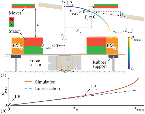
Figure 2.
(a) Section view of a radial displacement of the mover under destabilizing magnetic forces without active control. (b) The forces that the mover experiences can be measured as reaction forces on the stator and converted using a linear equation to extract the mover’s position for active position control. For the sake of illustration, the EMs’ return current path (see Figure 1) is not shown, and the levitation height is shown reduced compared to the other dimensions, which are drawn to scale.
Design optimization of stiffness for various DOFs was conducted in [28]. The method used involved setting a lower bound on the rotational stiffness of the mover to make it less prone to rotations due to external disturbances or during active control of radial movement. Conversely, for radial stiffness, a low value is beneficial for active control since less radial force is needed to keep the mover radially centered. However, trade-offs were required when choosing these two quantities since increasing the rotational stiffness reduces the levitation height, and reducing the radial stiffness proportionally reduces the passive axial stiffness, which needs to be large to improve the rejection of external disturbances acting in a vertical direction. Another important aspect to consider during the design of the PMs is robustness, which can be interpreted as the maximum displacement or angle that the mover can experience from its natural orientation and position (horizontal and radially centered) without changing its passive stability properties. To illustrate the concept of robustness applied to radial displacement, we consider the designed mover with three passively stable DOFs at in Figure 2a (including axial z movement and rotations around both radial axes, ). The mover can shift to ( while maintaining the same passively stable DOFs. Correspondingly, the axial robustness is measured by displacing the mover toward the stator starting from until a passive stability change is observed. This change occurs at , where an axial instability is observed (the mover is attracted by the stator). Knowing this levitation height and calculating the corresponding axial force determines the maximum payload the mover can carry, resulting in kg. Regarding the rotational robustness at (without payload), the mover can be rotated around the radial axes x and y up to 25°. For larger angles, the passive rotational stability is lost. These large robustness bounds enable the stabilization of the mover using the same control architecture under external disturbances and different payloads added to the mover. However, for the sake of demonstration, this paper focuses on the active control of the mover using a force sensor within a relatively small range around the natural levitation point , where the mover is unloaded and radially aligned with the stator.
When moved from the center, the mover is tilted, as depicted in Figure 2a, without active control. From the natural position , where the radial forces are theoretically zero, the levitating magnet starts moving along the colored trajectory, e.g., due to a slight asymmetry in the construction of the PMs, which is arbitrarily chosen to be in the positive x direction. The radial magnetic force on the mover is positive, meaning that the mover tends to roll away from the initial position and simultaneously rotates by an angle around the perpendicular y axis due to a passive magnetic torque acting in this direction. By taking a snapshot of the mover’s displacement and rotation (e.g., at position ), it can be observed that there is only the force , whereas the torque acting on the mover is , making it stable against rotations around the radial axes. Accordingly, the mover keeps a steady-state angle if controlled at a certain radial position . Therefore, the use of a force sensor for determining the mover’s position is an attractive option because of the linear relationship between the radial force and radial position, as depicted in Figure 2b, for a relatively broad radial range, considering that the mover is typically controlled at and . The magnetic force that the mover experiences when it is not radially centered is also observed as a reaction force on the stator with equal magnitude but opposite direction, meaning that the mover’s position can be indirectly measured using a force sensor, e.g., placed underneath the stator (see Figure 1). The force sensor discussed in this paper is a three-axis load cell employing strain gauges to measure the change in resistance due to the elongation and/or shortening of the gauges, which are glued to the deflecting aluminum elements of the sensor. With this sensing principle, the stator (placed above the sensor) must be able to move when radial forces act on the mover, as illustrated in Figure 2. To allow only radial movement of the stator with preferably minimal rotation, rubber supports are mounted below the stator’s mounting plate and fixed to a steady structure. The impact of these supports on the dynamics of the stator is modeled and calibrated using measurements (see Section 4).
Furthermore, the EMs used for the mover’s active stabilization are placed on the stator level to preserve the large levitation height h and are attached to the stator PM mounting plate so that the electromagnetic forces between EMs and the stator PMs do not act on the force sensor. Otherwise, if the EMs were placed near the stator PMs but mechanically decoupled, large electromagnetic forces between the EMs and stator PMs could saturate the force sensor.
3. Dynamics Modeling
This section describes the theoretical model of the MLP for active position control on the radial x axis for . The same considerations hold for the other radial y axis (and ) since the MLP is axially symmetric. The only differences, as explained in Section 4.2, are due to the asymmetrical construction of the force sensor.
3.1. Radial Motion Dynamics
As observed in Figure 2b, the magnetic force acting on the mover for a positive radial displacement is positive, and it is shown over in Figure 3b as a dotted red curve, calculated using the method proposed in [28]. In the neighborhood of the desired levitation point for the mover, where and , the simulated curve is linearized by a tangent line (centered at the origin and having the same slope as at ), which defines the radial stiffness, i.e., the proportionality constant between the displacement and magnetic force, denoted as , with its value given in Table 1 (note that indicates missing natural stability). The force generated by the electromagnets is measured using a force sensor by positioning the mover radially centered with the stator and varying the control current. The results are shown in Figure 3c. Both EMs that can generate a force in the x direction are used with opposite currents, and (see Figure 3a). One EM drags and the other pushes the mover, with the convention that a positive force causes a positive movement () generated by a positive current. For the given position of the mover, linearization to find is not needed since the EMs’ magnetic flux density on the mover is directly proportional to the current (Biot–Savart law), and the corresponding Lorentz force is, in turn, directly proportional to the magnetic flux density [28]. Another contribution to the total radial force experienced by the mover is the force related to the mover’s rotation , e.g., due to the unstable radial motion (see Figure 2). The curve obtained using the model in [28], as shown in Figure 3f, is linearized around and to obtain the constant . Accordingly, the linear equation of motion that describes the radial displacement of the mover under magnetic and electromagnetic forces in the neighborhood of and can be written as
where is the mover’s mass and t indicates the time. To derive the transfer function of the mover’s radial dynamics, we set and apply the Laplace transform to (1) using the complex variable s. This yields
which shows the instability of the model for radial movement due to the presence of a real right-half-plane (RHP) pole . In fact, when a positive current step is applied to the system with the mover initially centered, the trajectory becomes positive due to the positive electromagnetic force and continues to increase exponentially over time due to the positive magnetic force. For completeness, a block diagram of (1) (also valid for small ) and a Bode diagram of (2) (only valid for ) are shown in Figure 4b, where the natural frequency of the radial displacement of the mover is also shown, which is defined as
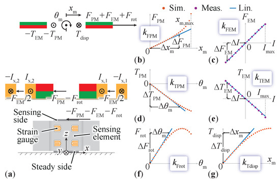
Figure 3.
(a) Section view of the MLP with the mover in the center, , and the force/torque vectors acting on the different parts of the MLP when a current I is injected into the EMs. (b–g) Linearizations of different simulations and/or measurements performed on the MLP according to Table 1, aimed at building a model in the neighborhood of , , and .
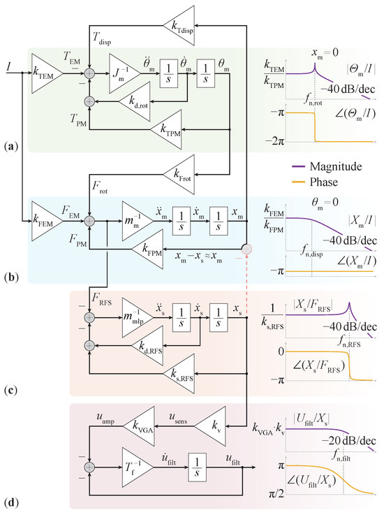
Figure 4.
Complete block diagram of the MLP, with the dynamics of the subsystems represented as Bode diagrams: (a) mover tilting and/or rotation, (b) mover displacement, (c) force sensor’s sensing element mechanical characteristic, and (d) force sensor mechanical-to-electrical signal conversion, amplification, and filtering. Parameter values are specified in Table 1.
The basic model described by (2) could be used to design a controller if the mover’s position is measured directly with a position sensor (see Section 4.1).
3.2. Rotational Dynamics
The force sensor’s reading also depends on the mover’s rotation . Therefore, a more sophisticated model of the mover’s motion is required because the mover may deviate too far from the reference center point and start to tilt around the y axis, as depicted in Figure 2a. In particular, this tilting can lead to an incorrect reading of the radial position, leading to incorrect compensation force generation by the EMs and potential instability of the mover. Due to its low rotational stiffness, the mover could also start tilting due to the torque generated by the EMs while trying to keep the radial position at zero. The current-dependent torque with the proportionality constant , as shown in Figure 3e, is calculated using the model extended to include the EMs [28]. This calculation is also proven with an alternative technique, as described below, where the difference between the two methods is within 8%. The alternative approach involves fixing the mover (in the radially centered position) along the y axis so that it can freely tilt around that axis without displacements while injecting constant currents into the EMs. For each current, the mover stabilizes at a certain angle because it is stable against tilting and/or rotations around the radial axes. The angle depends on the rotational stiffness, which is defined as the slope of the dotted curve in Figure 3d around the origin. In the reached equilibrium position, the tilting angle can be measured, and the EM torque can be found. This torque is known to be compensated by the PM torque (i.e., ), which is calculated as described in [28]. Another contributing factor to the total torque experienced by the mover is the torque related to the mover’s radial displacement . Correspondingly, the curve depicted in Figure 3g is linearized around and to obtain the constant . Accordingly, the linear equation of the mover’s rotation around the radial axes under PM and EM torques in the neighborhood of and can be written as
where is the mover’s moment of inertia and is a strictly positive damping constant for the rotation. This constant arises from the magnetic interaction between the stator and mover, giving rise to eddy current and hysteresis losses in the PMs [29]. In the s domain, (4) with results in
showing that the model for rotation is stable because of the positive coefficients in the denominator (Routh–Hurwitz criterion). However, depending on the constant , the rotation can be underdamped, as shown in the Bode diagram in Figure 4a, meaning that oscillations can occur at the natural frequency
With this extension of the mover’s dynamic model, a controller that stabilizes the mover in the radial direction and dampens the eventual rotary oscillations can be designed given the position and the rotation , as shown in Section 5.2.
3.3. Force Sensor Mechanical Dynamics
When the force sensor is used for position sensing, an extension of the MLP’s dynamic model is required to include the force sensor’s dynamics. This extension is presented below. As illustrated in Figure 2a, when the mover is radially displaced with respect to the center position, a reaction force acts on the stator, which can be assumed to be linearly dependent on the displacement for small deviations, i.e., . In addition, two more forces act on the sensor, i.e., the reaction force from the electromagnets and a force due to the tilting of the mover , as depicted in Figure 3a. The electrical signal provided by the force sensor is proportional to the elongation and/or shortening of the strain gauges and, therefore, to the movement of the sensing side of the force sensor (see Figure 3a), defined here as , which is caused by the total dynamic force
The transfer from the applied force to the linear movement of the force sensor can be modeled as a mass-spring-damper system (which is commonly seen in the literature [30,31,32]), using the following equation of motion
where is the total mass applied to the force sensor, comprising the mass of the PM stator, four EMs, the mounting plate, and the mover. denotes the viscous damping for the force sensor and is a strictly positive constant, and denotes the stiffness of the force sensor, determining how much the sensing elements bend under constant loads. In the s domain, (8) results in
which shows that the model of the force sensor is stable because of the positive coefficients in the denominator. Also, in this case, the sensor is prone to oscillations at its natural frequency
which depend on its damping constant , as illustrated by the peaking in the Bode diagram in Figure 4c. In addition, the total force acting on the force sensor causes the tilting of its sensing part and the whole mounting plate, which is attenuated by the rubber supports shown in Figure 2a. This hardware assembly slightly increases the stiffness of the force sensor since the low stiffness of rubber combines with the large stiffness of aluminum. Importantly, this avoids the need for a more complex model to account for the rotation of the PM stator and EMs around the radial axes. Both stiffnesses are included in the coefficient value in (8).
3.4. Force Sensor Electrical Dynamics
The electrical signal provided by the force sensor depends on the sensitivity of the strain gauges for a given mechanical stiffness, the gain of the electrical circuit, and the optional electrical filter used to attenuate high-frequency noise or electrical disturbances in the system. Therefore, a first-order low-pass filter transfer function combined with an inverting amplifier gain is used for the model. Additionally, the mechanical-to-electrical signal conversion is modeled with a constant gain , which leads to the following transfer function
where the cutoff frequency is equal to
For completeness, the time-domain representation of (11) is given as
and it is depicted in Figure 4d. The gain can be determined by displacing the mover in the vicinity of the levitating point by with and while measuring the electrical response of the force sensor. With prior knowledge of the sensor’s stiffness , the mover’s radial displacement stiffness , and the electrical amplification factor , the gain is obtained as
Strictly speaking, the gauges have specific dynamics since their stretch cannot happen instantly. However, these dynamics are simplified here with the constant since, according to the design, the stretching occurs almost simultaneously with the bending of the sensing element [33], which is limited by the frequency . The electrical amplification is simplified with the constant since the chosen cutoff frequency of the filter is much lower than the electrical bandwidth of the used amplifier, which lies in the megahertz range [34]. Furthermore, it is important to note that the overall sensor’s bandwidth, i.e., the dB frequency of the transfer function , must be sufficiently larger than the other characteristic frequencies in the system ( and ) in order to correctly measure the position and tilting-dependent forces of the mover without excessive phase shift. Otherwise, incorrect estimations of and can occur, leading to incorrect EM forces defined by the controller that would ultimately destabilize the system.
3.5. Summary of the Dynamics
The dynamic Equations (1), (4), (7), (8) and (13) are shown in the form of a block diagram in Figure 4, where the single input is the current I through the EMs and the single output is the amplified and filtered voltage of the force sensor . In the diagram, a simplification can be made assuming that the movement of the stator is negligible compared to the mover’s radial movement (red dashed connection in Figure 4). Strictly speaking, holds, assuming that the sensing side of the force sensor moves. However, given any mover’s position and knowing that the same magnetic force acts on the stator, its displacement can be calculated as , with the constants given in Table 1. Therefore, the stator’s displacement contribution to the magnetic force is small and can be neglected, i.e., the simplification is justified. Correspondingly, the complete and simplified model of the MPL is expressed using the following state-space equations:
with the input, output, and state variables:
and the corresponding matrices:
The Bode diagram of the transfer function
for currents through the EMs with different frequencies while the mover levitates around the center position is shown in Figure 5. In addition, the poles (seven in total) of the transfer functions (2), (5), (9), and (11) are shown with their real and imaginary parts. The diagram clearly shows two magnitude peaks at and , resulting from poles that possess a larger imaginary component relative to their real component. Additionally, the noticeable dip near is attributed to a pair of zeros located very close to the poles, indicated by green dots.
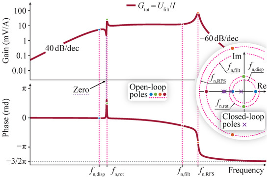
Figure 5.
Bode diagrams of the model for the MLP (see Figure 4). The inset shows the location of the seven poles of the system in the complex plane. A single pole is in the RHP and corresponds to the radial displacement of the mover (see (2)). The poles describing the mover’s rotation and the force sensor’s dynamics are stable but show a relatively large imaginary part, implying oscillations in the system. The magnitude and frequency axes are presented on a logarithmic scale.
4. Dynamic Model Verification and Tuning
To validate the complete dynamic model of the system in a first step, a measurement of the total transfer function has to be performed, where the stator PM and the EMs are mounted on the force sensor, and the mover levitates at the reference operating point while being able to move and tilt freely. For this purpose, an optical position sensor with sufficient bandwidth (at least ten times higher than , e.g., kHz [35]) directly measures the mover’s position and feeds the signal to a position controller that stabilizes the mover. In addition, sinusoidal currents are injected into the EMs, which excite the mover’s radial x position around the levitating point. At the same time, the electrical output of the force sensor is recorded. This method verifies the total transfer function depicted in Figure 5 (cf. Figure 7).
4.1. Mover’s Position Controller
A position controller that actively stabilizes the radial position of the mover is required for levitation at the desired operating point. Furthermore, the method for position sensing has to be preferably independent of the mover’s tilting around the radial axes such that only the part of the model described in Section 3.1, which pertains to radial motion, e.g., along the x axis, can be used to design the controller. Consequently, if tilting of the mover still occurs, it does not detrimentally influence the sensor readings and is naturally damped by passive magnetic interactions. The proposed approach, depicted in Figure 6, uses a PD controller, which stabilizes the mover’s radial displacement along the x axis by shifting the unstable pole to the left half-plane (LHP), combined with a PI controller, which enables steady-state reference tracking. To verify the dynamic model of the complete system, including the force sensor, the position signal is directly measured using an external optical sensor (Baumer OM70-P0140.HH0130.VI, [35]) and then filtered with a first-order low-pass filter . Using the straightforward method proposed below to design both controllers, a phase margin of about 52° at the desired crossover frequency is guaranteed. Nevertheless, other approaches can be implemented to achieve the desired system response, e.g., implementing and tuning a single PID controller. Stabilization can be achieved by measuring the position , differentiating it to obtain the mover’s velocity, and injecting a stabilizing current into the EMs proportional to these two quantities. Thus, (1), with the simplification , is extended to
where and are the proportional and derivative gains of the PD controller, respectively. It must be ensured that the measured mover’s position and speed are equal to the actual ones, i.e., and , for frequencies below the force sensor’s bandwidth (or the cutoff frequency of the measurement filter ), which should be ten times higher than the natural frequency of the mover’s dynamics as a commonly used guideline in control systems. Therefore, in the following analysis, it is assumed that the sensor’s dynamics have no impact on the design of the controller. In the frequency domain, the transfer function from the EMs’ current to the mover’s position can be expressed as
and has two stable poles if and only if the coefficients in the denominator are strictly positive (Routh–Hurwitz criterion), meaning that the minimal requirements and must be satisfied. This also shows that a derivative controller must be implemented; otherwise, when , either an unstable real pole still exists for or two purely imaginary poles are obtained if the mentioned requirement for the proportional gain is fulfilled, leading to oscillatory behavior. Furthermore, comparing the denominator of (25) with the standard form of a second-order system:
where is the natural frequency and is the damping ratio, expressions for the PD controller gains can be obtained
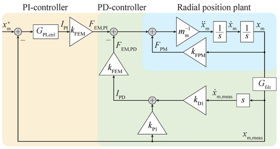
Figure 6.
Block diagram of the mover’s position control built with a PD controller that stabilizes the unstable radial dynamics and a reference tracking PI controller.
It can be seen that the aforementioned basic requirements are satisfied regardless of the chosen natural frequency and damping ratio, meaning that a stabilization of the mover is theoretically always possible for each pair . For the sake of simplicity, the PI controller can be designed as
such that its corner frequency is the same as the chosen natural frequency for the stabilized plant given by (25), i.e., . Its constant gain is the inverse constant gain of (25), leading to the following equations for the controller gains
Eventually, by multiplying (25) and (29) with the corresponding gains from (27), (28), (30) and (31), the expression
is obtained. To show that the afore-mentioned phase margin at the desired crossover frequency can be achieved, the damping ratio has to be chosen as
so that a critical damping of the PD controller stabilized plant (25) is obtained, indicating no overshoots or oscillations while stabilizing the mover’s position are expected. Accordingly, (32) can be rewritten as
The crossover frequency is found at the frequency where the magnitude of (34) is unity by substituting the complex variable , i.e., solving
for . The only positive and real solution that can be found is
which means that the crossover frequency is linearly dependent on the natural frequency and can be arbitrarily chosen. Consequently, the phase of the open-loop transfer function at the crossover frequency can be calculated as
and is independent of the chosen crossover or natural frequency, meaning that the phase margin is always given as
Finally, the closed-loop transfer function that defines the response of the controlled system is given as
and shows a typical second-order system response when comparing its denominator with (26), where the natural frequency (or bandwidth) is and the damping ratio is , meaning that an overshoot in the mover’s position is expected when the controller is trying to track, e.g., a step reference signal .
In summary, the only parameter that has to be chosen using the proposed design technique is the bandwidth of the closed-loop system . Together with the requirement of (33), the four controller gains (27), (28), (30) and (31) can be calculated. Note that a trade-off between fast dynamics and the required control current has to be made. Choosing a large bandwidth automatically leads to an increased EM current because all controller gains are dependent on , and they determine the required current depending on the mover’s position and velocity, as shown in Figure 6. Therefore, the maximum achievable bandwidth depends on the current limit, which should not be exceeded to ensure a proper controller function and is usually given by the power electronics that supply the current to the EMs.
4.2. Dynamic Model Proof and Adaption
For the verification of the dynamic model of the system, a measurement of the transfer function in the frequency domain from the EM current to the force sensor output is performed on the x and y axes individually. Here the mover is free to travel on the investigated axis while its movement is restricted on the other axis with a customized barrier that allows sliding with little friction (see Figure 7a). For this preliminary test, the mover is actively controlled on the investigated axis in the radially centered position, using an optical sensor [35] placed at the mover’s level, which enables measuring the position with 10 accuracy. The controller is implemented using the structure discussed in Section 4.1, where the only design parameter is the closed-loop bandwidth, which is chosen to be . Higher controller bandwidths up to have been tested, but the system was more prone to vibratory behavior. To record the desired transfer functions, sinusoidal currents at different frequencies are added to the control currents and injected into the EMs (see Figure 7b) to cause a displacement of the mover in the neighborhood of the levitation point of the investigated axis, and all reaction forces on the stator are measured using the force sensor.
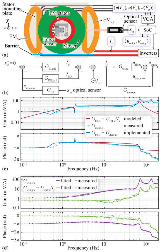
Figure 7.
(a) Top view of the measurement setup to verify the MLP’s dynamic model in the x direction. The mover’s position is controlled based on optical position measurement, and sinusoidal currents are injected into the EMs to cause a displacement of the mover. Consequently, a reaction on the stator is measured using the force sensor while the y position is kept constant at with sliding barriers. (b) Block diagram of the control system depicted in Figure 6 that levitates the mover. Currents are summed to the control currents to verify from Figure 5 by measuring . (c) Frequency responses of the model, measurement, and disturbance-corrected output of the force sensor along the x axis in response to an input current in the x direction (with mover levitating). (d) Model disturbance and cross-coupling between the y-axis current and the x-axis sensor output (without the mover). Please note that the measured phase lies within but has been unwrapped for this representation (i.e., adjusted by adding or subtracting to targeted phase values to ensure a continuous and smooth representation without discontinuities).
As schematically shown in Figure 7a, the electrical signals from the force sensor are amplified, filtered, and stored on the SoC as and (the subscript letters and are introduced to distinguish the quantities between the axes). Ideally, the voltage should be determined by multiplying the theoretical system’s transfer function with the EMs’ current (i.e., without disturbances , as shown in Figure 7b, ). The voltage should ideally be zero across all frequencies, with the assumption that no cross-coupling between and exists. Additionally, the current is calculated as the mean value between the individual EM currents, i.e., , where the negative sign accounts for the opposite directions of the currents in the two coils of an axis (see Figure 1), which generate a force on the mover in one direction.
The resulting measured system’s transfer function of the preliminary test on the x axis is shown in Figure 7c as a series of cyan points within the frequency range of . The gain and phase were calculated over at least eighteen periods for the lowest frequency and up to fifty for the largest frequency. When comparing the measurement with the theoretical transfer function (solid red line) shown in Figure 5, a good agreement can be observed from the natural frequency of the mover’s rotation (tilting) up to the force sensor’s natural frequency at . At these resonant frequencies, the constants , , and are finely tuned to match the measured peakings, resulting in the values reported in Table 1. During measurements in this frequency range, the mover experiences a small displacement from the radially centered position, up to 1 mm for the lower frequencies. Additionally, a rotation around the y axis can be observed, along with vibratory behavior ranging from 6 Hz up to 10 Hz. The mover holds its centered position for larger frequencies because of its large inertia, which prevents larger movements, meaning that only the reaction forces caused by the EMs are applied to the force sensor, as PM forces would only occur for a finite displacement and/or rotation of the mover. For frequencies lower than 2 Hz, during which the mover is displaced up to 4 mm from the center, there is a mismatch between the model and the measurements. The dip in the transfer function at Hz due to the cancellation of all reaction forces, as illustrated in Figure 5, is still visible, but the increasing gain connected to a phase equal to zero in the lowest frequency region could not be measured in the real system. Another discrepancy with the model is found at frequencies larger than 70 Hz due to a vibratory mode of the whole mechanical system, with a prominent peak near 130 Hz. This behavior is commonly found in complex mechanical structures involving multiple parts [36]. In summary, the important characteristics of the theoretical model are visible in the measured transfer function. However, some deterministic behavioral differences must be addressed before the force sensor’s signal can be used for the feedback control of the mover.
These differences are visible when performing the second measurement, wherein the mover is removed from the system and sinusoidal currents are injected into the EMs (as with the first measurement, each axis is considered individually). According to the model depicted in Figure 4, the force sensor should not register forces since all reaction forces from the mover (, , and ) are zero. Accordingly, the electrical signal should be zero regardless of the injected current. However, as shown in Figure 7d, transfer functions with gains comparable to the modeled transfer function are measured. represents the disturbance on the modeled function and is obtained by injecting into the EMs and measuring without the mover. Therefore, it differs from the measurement with the mover levitating, as depicted in Figure 7c. Nevertheless, it can be seen that the two peaks around 70 Hz and 130 Hz are still visible, indicating that forces are acting on the force sensor. These forces originate from the electromagnetic reaction between the EMs and the PM stator. They generate a displacement of both objects (EMs and PM stator) on the stator’s mounting plate due to poor mechanical mounting, resulting in movement of the force sensor’s sensing side. This effect is also observed at the lowest frequencies, which explains the relatively large gain compared to the model. Furthermore, in the frequency range above 1 Hz, another effect that directly affects the strain gauges is observed, namely induced voltages, which are summed to the force-dependent voltages and are caused by the time-varying magnetic fields from the electromagnets. The origins of both disturbances can be proven by removing the PM stator from the system, where only the induced voltages can be measured with a phase of with respect to the current in the EMs. Eventually, by fitting the measurement of with the transfer function estimation tool provided by MATLAB® and adding the obtained frequency response to the model transfer function , the measurement performed with the mover levitating can be reproduced with better accuracy (cf. with in Figure 7c). The error that remains between the transfer functions can be attributed to the fact that the two measurements (with and without the mover) are performed separately, and the model parameters also contain errors originating from their measurement and/or simulation. Another behavior that is hard to model but is prominent in the output of the force sensor, as shown in Figure 7d, is the cross-coupling between the axes, which is represented by the transfer function for the force sensor’s output due to a current when the system is excited without the mover. For this measurement, the same disturbances as those observed for are visible, where the movement of the stator and EMs in the y direction causes a false reading in the x direction, and vice versa. In this measurement, the amplitude of the disturbance on the sensor output is slightly above the noise level for the lower frequency range. Between 10 Hz and 25 Hz, only noise is measured, as can be seen in the distribution of the measurement points, especially in the phase plot.
The same measurement procedure is performed to characterize the y axis of the sensor, where similar results are expected due to symmetry. However, a small difference is observed in the sensor’s natural frequency ( compared to ) due to the different stiffnesses of the sensing elements, along with a 25% higher damping coefficient. Therefore, an adaption of the theoretical model (15) regarding the sensor’s parameters is performed, leading to a correspondingly different model transfer function . Furthermore, a comparable yet dissimilar disturbance profile is observed, resulting from the aforementioned disturbance influences. Finally, a transfer function is used to consider the model disturbance on the y axis from the y current, and accounts for the cross-coupling originating from the x current.
5. Observer and Controller Design
5.1. Observer
The proposed position-sensing method uses a force sensor to detect the forces due to the mover’s motion, which are then translated into the position using the model and calibrated disturbance transfer functions. These calculations are performed by an observer that estimates the states of the system based on the input variable, i.e., measured EMs’ current , using (15). Moreover, the observed states are corrected with a state correction architecture (which is required to address model mismatches and noise) by comparing the calculated output (16) to the measured output . If the observer and the real system react the same way to an input current, the error between the estimated output and measured output would be zero, meaning that the calculated mover’s dynamic behavior is the same as that in the real-life hardware demonstrator. However, as seen in Figure 7c, there are relatively large mismatches due to the disturbances between the theoretical model and measurements. Thus, a correction of the observed states has to be performed so that the output of the observer ultimately matches the measured output. Therefore, to minimize the observer’s state errors, a dynamic model that matches the measured transfer function depicted in Figure 7c has to be implemented on the SoC. As argued in Section 4.2, the disturbance of the model is completely decoupled from the mover’s dynamics. Hence, it can be used to better estimate the real output of the force sensor by summing its response with the response of the original model , as schematically shown in Figure 8. This way, the original seven states are still corrected with the feedback architecture of a Kalman filter, as described in [37], whereas the model disturbance is used as a feedforward block that directly affects the observer’s output . Furthermore, the cross-coupling function is incorporated into the observer as an additional feedforward block to enhance the tracking of the states since all non-ideal disturbances are considered in calculating the estimated x-axis force sensor’s output, which depends on the currents on both axes. The same observer structure is implemented for the y axis, incorporating the discussed calibration-based improvements of the model, like the measured disturbance and cross-coupling transfer functions. Accordingly, the observed outputs for both axes are written in the s domain as
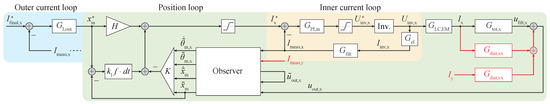
Figure 8.
Block diagram of the MLP with the mover’s dynamics observer, position, and current controllers for the x axis. The black boxes represent the ideal MLP as presented up to and including Section 3, whereas the red boxes are required to extend the model for the realized prototype discussed in Section 4.2 so that the observer delivers the states as close as possible to reality for the position controller. For these disturbance corrections, the y-axis current plays a role in the x-axis model, and vice versa.
5.2. Mover’s Position Controller and Rotation Damping
As discussed in the previous sections, the magnetic levitation platform requires at least active control of the mover’s radial position since it is intrinsically unstable. However, an active contribution to damping other stable DOFs might also be required, especially when the mover oscillates due to poor passive damping. In addition to stabilizing the mover’s radial position, as described in Section 4.1, the proposed controller actively dampens any eventual rotary oscillations. Therefore, the mover’s position and tilting angle must be measured. As seen before, to stabilize the radial position, the velocity is required, whereas for the active damping of the rotation, the angular speed is necessary. Advantageously, both can be found from the derivatives of the position measurements and over time. The proposed approach is a state-space (or time-domain) stabilizing controller based on a reduced state-space representation of the MLP that only considers the mover’s dynamics. The force sensor’s mechanical and electrical dynamics must not be controlled since the movement of the sensing side is relatively small and has practically no impact on the magnetic forces. Accordingly, the model assumes that the observed quantities (, , , ) are equal to the real-life quantities (, , , ) and it is expressed as
with the input, output, and state variables:
and the corresponding matrices:
This representation can be used independently of the position-sensing method as long as the position and the rotation are obtained. As already mentioned, the mover’s velocity and angular velocity can be calculated by differentiating the position and the angle. The controller, in the form of a matrix K, uses all available information, in this particular case, derived from the observer (see Figure 8), and calculates the current
which stabilizes and dampens both mover’s dynamics (note ; see (17)). The value of the controller gains can be found, for example, using the linear quadratic regulator (LQR) algorithm [38], which is widely used in the literature [39,40,41]. This results in the optimal input following the control strategy (50), which minimizes the cost function
where Q is a symmetric and positive definite matrix and R is a strictly positive weighting constant. The state-space matrices and , along with Q and R, define the control matrix K by solving the continuous-time algebraic Riccati equation for the matrix P, expressed as
For the design of the stabilizing controller component, a choice of weights has to be made, as shown in Section 6.2, where the single states and the input variable can be penalized in the cost function. This allows the algorithm to find a controller that ensures strong damping of rotation while keeping the mover stable in the radial direction. As a consequence, the unstable pole due to the radial magnetic forces is shifted to the LHP, and the imaginary component of the rotation-related poles is reduced so that all four poles lie on the negative real axis or as close as possible to it, as depicted by the violet crosses in the complex plane in Figure 5. Furthermore, the stabilizing controller component is extended with a reference tracking system [42], consisting of a proportional and an integral part, as illustrated in Figure 8. This system enables tracking a reference radial position , which is normally set to zero so that the mover is kept radially centered, assuming that the position signal has no offset. Conversely, rotation (tilting) tracking is not implemented since the reference mover’s angle is zero, corresponding to the natural angle when centered. The proportional controller consists of a constant H chosen such that at steady state (i.e., when ), the position of the mover is equal to the reference value with the extended control strategy
Therefore, the set of equations
has to be solved for H, leading to the result
The integral controller is required to ensure that the reference signal is tracked without steady-state errors, thereby extending the control strategy to
where is the integral gain, which should be chosen relatively low to avoid interference with the stabilizing controller during transients caused by external disturbances on the mover position. The resulting values for the control matrices and constants are listed in Table 3.
5.3. Inverter Stage
So far, it has been assumed that the current in the EMs is readily available and can be directly adjusted by the position controller and active tilting damper. However, in reality, a voltage U must be first applied to the EMs’ terminals, which, together with the resistance and inductance , determine the transient behavior and steady-state value I of the current. Therefore, a current controller that dynamically sets the proper voltage depending on a reference current value from the position controller and active tilting damper has to be designed. This can be achieved with a cascaded structure, as shown in Figure 8. It must be ensured that the bandwidth of the inner current loop is sufficiently higher (e.g., ten times larger) than the bandwidth of the position controller and active tilting damper so that the dynamics of the current control need not be considered during the design of the position controller and active tilting damper, for which we assume . In the simplest case, the voltage applied to the EMs is the average value of a switched voltage generated with an inverter block (e.g., a full-bridge inverter) that allows generating positive () and negative () voltages out of a constant-voltage source , as indicated in Figure 1. However, due to the large that modern power semiconductors can generate while switching, a filter at the output of the inverter stage is required. Without the filter, the high-frequency components of the switched voltage ( in Figure 9) would drive a high-frequency current , which finds a low impedance path through the parasitic capacitance of the EMs. The return path for this current is via the EMs’ cables, modeled by the impedance , and via the ground connection of the position measurement circuit, modeled by the impedance , which includes the aluminum body of the force sensor, the conductive shield of the force sensor’s cables, and the reference potential for the measurements. Due to their close placement, the position measurement circuit is coupled with the parasitic capacitance to the corresponding EM and is tied to the common ground on the inverter. Furthermore, the time-varying common-mode voltage induces a common-mode current in the cables of the EM that charges and discharges the coupling capacitance (see Figure 9). Both currents, and , can generate an error in the position measurement since the analog voltage, which is then sampled by an ADC, is not only determined by the amplifier circuit modeled by the gain but also by an error voltage, i.e., . To minimize these noise issues, we employ a passively damped filter. This filter reduces the amplitude of the high-frequency current flowing through the EMs, which eventually reaches the position measurement circuit because of their close placement within the MLP. It achieves this by providing a low-impedance return path via the filter capacitors and . Furthermore, we add a common-mode choke that increases the common-mode impedance of the load at the output of the inverter to reduce the amplitude of the common-mode current. For the design of the filter, we follow the commonly used guidelines described in the literature [43] to optimally dampen the filter and avoid resonances with the driving converter. The first consideration is to achieve a large high-frequency attenuation (>40 dB) at the switching frequency , as reported in Table 2, meaning that the design frequency, which is given as
has to be at least ten times lower than the switching frequency since the filter’s roll-off is . The second consideration is that for strong resonance damping, a large ratio
is favorable in combination with the optimally designed damping resistor [44], calculated as
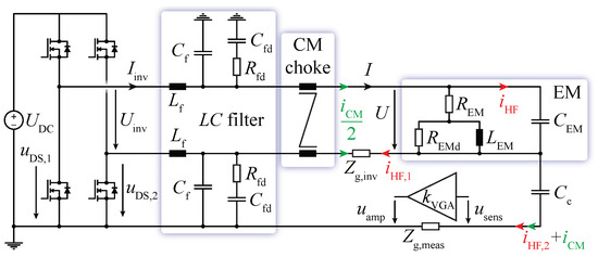
Figure 9.
Electrical system consisting of a full-bridge inverter driving the EM of an axis. A passively damped filter is inserted to reduce the disturbance , which can affect the position measurement circuitry due to coupling denoted by with the EM, modeled by four lumped elements. Similarly, the common-mode choke helps reduce the amplitude of the high-frequency common-mode current .
Table 2.
Parameters of the inverter, filter, and EM equivalent circuit shown in Figure 9.
Regarding the controller design, the proportional and integral gains of the PI controller are calculated using the MATLAB® function “pidTuner”, where the closed-loop bandwidth , given in Table 3, of the inner current control loop is selected according to the transfer function of the designed filter from the inverter voltage to the inverter current . As indicated in Figure 8, a filter on the feedback path of the inner current controller is used to better approximate the current in the EM from the measured current . To minimize the phase shift, its cutoff frequency should be larger than the desired bandwidth . For the controller design, the filter for the current is included in the open-loop transfer function , and care is taken to achieve a sufficient phase margin that avoids overshoots in the EMs’ current.
Table 3.
Parameters of the outer current controller, position and active rotation damping controller, and inner current controller.
Additionally, the minimum required DC voltage of the inverter depends on the required control bandwidth and the current amplitude necessary to counteract displacements of the mover. This is given by . For the selected and current amplitude corresponding to , a minimum is calculated, which must be achieved to obtain the desired dynamics of the current. This is related to the DC voltage applied to the EM, i.e., , assuming a purely inductive EM (see Figure 9 and Table 2). Finally, to achieve the maximum value of the current at steady state, a minimum DC voltage must be available at the EMs’ terminals. Further, the switching frequency should be chosen to maximize the efficiency of the inverter, considering the switching and conduction losses of the power transistors during operation. This choice has no impact on the operation of the MLP as long as it is ten times higher (as a rule of thumb) than the largest bandwidth in the system . Otherwise, proper current control cannot be achieved. The selected inverter voltage and switching frequency listed in Table 2 satisfy these requirements.
5.4. Position Sensor Offset Compensation
In cases where the measured or observed mover’s position signal has a constant or slowly fluctuating offset, e.g., due to temperature dependencies, the proposed controller would position the mover with a deviation of the reference position. Therefore, an outer current control loop (see Figure 8) is required to compensate for this offset. When the mover’s reference position is zero, the EMs’ current should also be zero since there are no radial magnetic forces that destabilize the mover. Otherwise, a control mechanism should drive the current to zero by setting a reference position for the mover that eliminates the position offset. This is achieved using a slow integral controller that adjusts the mover’s reference position so that the error between the reference current at the desired position of the mover and the measured current is zero. This works for any desired position of the mover since the required current that compensates for the radial magnetic force is known (either measured or calculated using a model). In the linearized model in Section 3.1, for the design of the controller gains, a plant with a constant relation between the mover’s reference position and the current flowing in the EMs
can be considered with the requirement that the outer current controller’s bandwidth is much lower than the dynamics of the position controller. Please note that the negative sign in (62) originates from the fact that a negative current must be generated to compensate for a positive magnetic force observed for a positive radial position. To fulfill the mentioned prerequisite, the integral controller is designed such that the closed-loop bandwidth results in a significantly lower value (e.g., ten times lower) than the lowest bandwidth in the system (see Table 3), i.e., the closed-loop bandwidth of the mover displacement, leading to
The closed-loop transfer function shows a typical first-order low-pass filter behavior with cutoff frequency (bandwidth)
With this design and the constraint on the bandwidth, there are no concerns about the phase margin and eventual dynamic overshoots since the assumed plant (62) is characterized by a constant value, and with an integral controller, the phase margin is at least °. However, when the bandwidth of the outer loop has to be increased for a faster dynamic application, care must be taken in the model of the plant (62) and the corresponding controller design by considering the dynamics of the position controller and, eventually, the response of the inner current loop.
Furthermore, even with the proposed offset compensation for the position sensor, a positioning error originating from an offset in the current measurement can still exist. Considering an error due to a constant offset in the position sensor and a position error due to a constant offset in the current sensor , the current error that leads to the same position error can be found as . Considering the case at hand and assuming that the position error is , the equivalent error of the current sensor would be . Therefore, employing an outer control loop is beneficial because most commercial sensors with current ratings are orders of magnitude larger than , resulting in greater accuracy. The used shunt resistor-based current sensor achieves an accuracy of 60 mA with a measuring range of 10 A, i.e., a % accuracy.
6. Hardware Demonstrator Realization
This section provides a detailed practical investigation of the MLP hardware demonstrator equipped with a (reaction) force sensor for the mover’s position sensing that proves the effectiveness of the previously discussed model, observer, and controller design. The properties of the passive part of the MLP, resulting from the design of the PMs in [28], including the determination of the mover’s levitation height and, most importantly, the radial destabilizing force that has to be counteracted by the EMs, have been discussed in Section 2. The design and optimization of the EMs are equally important since they define the final size of the MLP and the power consumption for achieving stable levitation, i.e., the copper loss per unit of radial displacement and unit of height. The dimensions of the EMs are chosen so that a large controllable range in the radial direction of the mover is possible while trying to keep the dimensions of the overall MLP as compact as possible. In addition, efforts are made to maximize force generation with the smallest possible amount of current (i.e., reduce power losses in the EMs). For more details, see Appendix A. Each of the four employed EMs (two for each radial axis) is driven by a corresponding full-bridge power electronics inverter (see Figure 9) with and a maximum output current of , which provides the required voltage to the EMs’ terminals. This voltage is calculated using an SoC featuring a CPU (where the observer and controller are implemented) and an FPGA, which provides the gate signals to the power transistors of the inverters and records the signals from the force sensor.
6.1. Force Sensor
The device used to sense the mover’s position in the MLP featuring extreme levitation heights is a force sensor. It is composed of a three-axis () strain-gauge load cell [45], rated for a maximum force of 100 N on each axis. Theoretically, only two axes () would be necessary to regulate the mover’s radial position. However, the additional sensing axis (z) is required for future applications not discussed in this paper, where the mover is loaded with a payload, and the levitation height can be determined by measuring the system’s total weight. Consequently, a force sensor with a notably high maximum force rating (100 N) is selected. This sensor is perpetually subjected to a load of N due to the mass of the stator (refer to Table 1 for numerical values). As a result, a margin of N is available to accommodate both the inertial forces and any additional payload. The force sensor provides an electrical signal of 1 mV/V at the rated force, meaning that for the chosen excitation voltage of 3 V applied to the strain gauges, a maximum signal of 3 mV can be measured at the sensing terminals. For displacement of the mover by 1 mm from the center, the magnetic force that has to be sensed is N, which corresponds to a voltage difference of V. Accordingly, an amplifier featuring very low noise levels is required to obtain a signal measurable by an analog-to-digital converter (ADC). The amplifier circuit depicted in Figure 10 consists of a buffered very low-noise constant-voltage reference (LTC6655 [46]) used to excite the strain gauges, which are arranged as a Wheatstone bridge for each axis, and three variable-gain amplifiers (VGAs) [34] that amplify and filter the differential signal from the gauge bridges. The cutoff frequency can be set using an external capacitor that builds a first-order low-pass filter using the internal feedback resistor . The voltage gain can be dynamically tuned from the SoC for applications where the mover changes levitation height (due to different payloads). In these cases, the amplification has to be changed to avoid saturating the VGAs’ outputs since larger radial forces, i.e., signals, are observed when the mover approaches the stator. Before the amplification, a manual offset compensation is implemented. This ensures that the force sensor output signal is set to zero when there are zero forces acting on the force sensor, as the strain gauges forming the Wheatstone bridge may have slightly different resistances, which could cause saturation of the output due to the high gain of the VGAs. Finally, the amplified and filtered analog signals are digitized by a multi-channel ADC [47] communicating with the SoC. It should be noted that for static applications, the implemented amplifier enables measuring forces with a resolution of mN, which translates to a positional accuracy limit of around 74 for the investigated MLP.
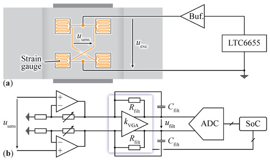
Figure 10.
(a) Excitation of the strain gauges, glued to the force sensor for a single axis, with a buffered constant-voltage reference. (b) Schematic circuit diagram of the force sensor amplifier for a single axis, consisting of a manual offset correction stage, variable-gain amplification, and analog-to-digital conversion.
6.2. Controller Tuning
With the correctly estimated quantities (, , , ) describing the mover’s motion, a state-space controller, as described in Section 5.2, is implemented for both the x and yv axes in the same way since it only depends on the mover’s parameters, which are equal for the x and y axes due to symmetry. For this purpose, the choice of the weighting matrix Q and the constant R for tuning the LQR controller is carried out so that the mover’s rotation (tilting) around the x and y axes is strongly damped. This is achieved by choosing a relatively large constant, leading to a reasonable distribution of closed-loop poles. Indeed, with
all poles of the closed-loop transfer function (i.e., the eigenvalues of the matrix ) lie on the negative real axis between Hz and Hz, as indicated in the s plane shown in Figure 5 with violet crosses, and reported in Table 3 as , , , and . Further, the integral gain that completes the mover’s position and rotation control law (58) is chosen to be equal to one-tenth of the smallest pole in the stabilized system (so it does not interfere with the stabilizing controller component), i.e., . Additionally, the filters for the inverter outputs (see Figure 9) are designed taking into consideration the volume of the passive components and the design guidelines introduced in Section 5.3, leading to the values listed in Table 2. The design frequency is , leading to an attenuation of 46 dB on the EM voltage at the switching frequency (100 kHz). The impact of the output filter on the EM current dynamics is very small, as the impedance of the capacitors is at least 10 times larger than that of the EM coils within the current control bandwidth of . The bandwidth is chosen to be as low as possible (i.e., about ten times higher than the highest frequency pole of the position controller) in order not to trigger vibrations of the mechanical structure since the output signal of the force sensor could be heavily disturbed by oscillations around 130 Hz (see Section 4.2). A measure that has been proven to work with a higher current-loop bandwidth (e.g., 100 Hz) is a moving average filter on the current reference signal calculated by the position controller and active tilting damper. The number of data points considered for the average is chosen to eliminate current components that would trigger a vibration of the structure. Due to relatively large noise on the force sensor signals and their slowly fluctuating offset, an outer current controller that drives the current to zero, thus centering the mover, is implemented following Section 5.4 with a closed-loop bandwidth of . The reported implementation works well for both axes, i.e., the mover never experiences rotary (tilting) oscillations, and its radial position is stabilized.
6.3. Results
A demonstration of the stable levitation is depicted in Figure 11, with the mover levitated at an air gap of 104 mm above the stator. The calculated standard deviation of the position recorded over ten seconds during the course of levitation is mm for the x position and mm for the y position, indicating that the mover experiences a certain deviation from the center and that the performance on both axes is similar. Furthermore, the effect of the controller that eliminates the force sensor’s offset is visible when comparing the mean values of the mover’s position and the EMs’ currents in the plot on the oscilloscope and in Figure 11b,c. The first is also depicted in Figure 11b. The second is , as also depicted in Figure 11c. Therefore, even though the observer calculates a position with an offset originating from the force sensor, the mover will be controlled in the center’s vicinity, where the magnetic forces, and hence the mean values of the control currents, are zero.
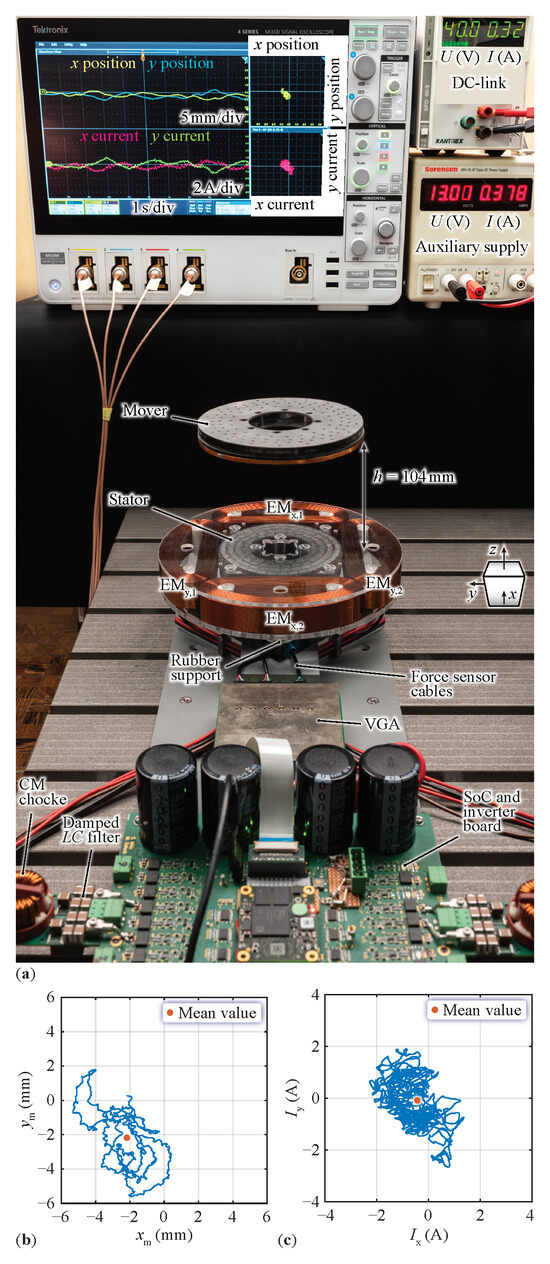
Figure 11.
(a) The complete system showing the mover’s stable levitation above the stator with a 104 mm air gap. The force sensor is not visible because it is placed underneath the stator and is connected to the VGA that amplifies and filters the force-dependent signals and delivers them to the observer implemented on the SoC. The DC-link supply is used for the EMs, whereas the auxiliary supply provides power to the SoC and the force sensor. (b,c) show the 2D plots of the observed mover’s position and control current, respectively, which are also found in (a) on the oscilloscope with a different scaling factor.
7. Conclusions
This work presents a novel method for sensing the position of the mover in a magnetic levitation platform (MLP), where a force sensor is used to detect the reaction forces on the stator. The force sensor enables the operation of the MLP in situations where the mover is encapsulated in a hermetically sealed chamber and levitated with an extreme air gap. An observer extracts the mover’s radial position and angle from the measured forces, which also depend on the control actions, to achieve closed-loop position control of the mover. For this purpose, a dynamic model of the MLP, including the force sensor, is developed and augmented to compensate for unwanted disturbances with a calibration procedure. Finally, based on the developed model, a state-space controller allows controlling the mover’s position and actively dampens eventual rotary (tilting) oscillations around the x or y axis.
With the proposed methods, a stable levitation of the mover is achieved, with an air gap of 104 mm, a characteristic dimension of , and a passive radial stiffness of the MLP of N/m. The performance is evaluated during centered () steady-state levitation by calculating the standard deviation of the mover’s position, which results in . To the best of our knowledge, the proposed MLP, along with its position control via stator reaction forces, is unprecedented in the existing literature. This novelty precludes direct performance comparisons with documented studies.
In future research, alternatively, eddy current measurements will be used for determining the mover’s position, and a comparative evaluation of the position control performance of both concepts will be provided.
Author Contributions
Conceptualization, R.B., L.B. and D.B.; methodology, R.B., L.B., S.M. and D.B.; software, R.B. and D.B.; validation, R.B.; formal analysis, R.B. and S.M.; investigation, R.B. and L.B.; resources, J.W.K.; data curation, R.B.; writing—original draft preparation, R.B. and S.M.; writing—review and editing, R.B., S.M. and J.W.K.; visualization, R.B., S.M. and J.W.K.; supervision, D.B. and J.W.K.; project administration, J.W.K.; funding acquisition, J.W.K. All authors have read and agreed to the published version of the manuscript.
Funding
This research was funded by the Else und Friedrich Hugel-Fonds für Mechatronik/ETH Foundation.
Data Availability Statement
Data presented in this study are available on request from the corresponding author.
Acknowledgments
The authors are very much indebted to the “Else und Friedrich Hugel-Fonds für Mechatronik/ETH Foundation”, which generously supported the research on magnetic levitation platforms with extreme levitation distance at the Power Electronic Systems Laboratory of ETH Zurich.
Conflicts of Interest
The authors declare no conflicts of interest.
Appendix A. Design of the Electromagnets
In this appendix, we briefly discuss the design considerations and resulting dimensions and properties of the electromagnets (EMs) employed in the magnetic levitation platform (MLP).
As a starting point, a constraint on the positioning of the EMs is set to preserve the levitation height obtained by the choice of dimensions of the permanent magnets (PMs). The EMs can be placed in a region below the top face of the PM stator in the vertical direction, e.g., around the stator, as shown in Figure 1, or between the stator and the force sensor. At least three EMs are required to control the mover on the 2D plane formed by the axes [48]. However, four EMs have been chosen so that both axes can be controlled independently and to facilitate the measurement procedure, using only two corresponding EMs for the dynamic model’s verification.
The realization of the EMs is constrained by the current and voltage of the power electronics inverter, the maximum RMS current density, and the dedicated space around the PM stator that has to be minimized to obtain a compact MLP with respect to its large levitation height. The readily available inverter board [49] used to demonstrate the functionality of the MLP provides enough integrated half-bridges (LMG5200) that can be combined to obtain the required number of full-bridge inverters for driving the EMs. The maximum allowed and selected DC supply voltage of the inverter board is , and the maximum current capability for each half-bridge is 10 A. However, a maximum allowed current of is chosen for the design of the EMs so that cooling the power semiconductors inside the LMG5200 can be avoided and their reliability is increased. It should be kept in mind that during nominal operation, only a small current is required to keep the mover at the natural levitation point. Larger current values are required during eventual transient periods occurring due to external disturbances.
The first important requirement for the EM design is to define the mover’s controllable range in the radial direction with respect to the center position , which determines the maximum magnetic force that has to be compensated by the EMs. This is chosen to be to provide enough room for characterizing the sensing system and corresponds to a force of . With the fixed controllable range, the optimization goal is to maximize with an optimal EM placement so that the current, current density, power losses, and driving voltage remain low. To achieve the minimum required current for the smallest EM, the size of the EM, and therefore, the characteristic dimension of the system (see Figure 1), is iteratively increased until the required force can be reached without exceeding the voltage, current, and current-density limits. Throughout the iterative process, the spatial constraints, such as the distance to the stator and adjacent EMs, are kept the same. Regarding the winding area, a height of is chosen to be equal to the stator’s height (considering an additional 3 mm separation for the plastic magnet holder) to achieve a compact design, and the width (see Figure 1) is iteratively increased with the characteristic dimension.
With all the above considerations, the final manufactured EMs exhibit a winding area of and , with a wire diameter of and insulation thickness. These parameters are listed in Table A1. The number of turns is , with 20 horizontal layers and alternating between 27 and 28 vertical layers using the orthocyclic winding style. The fill factor is , resulting in an approximate winding resistance of , which defines the minimum DC-link voltage as . Finally, the approximate weight per EM is . When comparing the force generation, the manufactured EMs have a simulated force constant of (as reported in Table 1), which is calculated from the sum of forces of each winding in the EM when two EMs per axis are used for control.
Table A1.
Parameters for the design of the EMs and their calculated characteristics.
Table A1.
Parameters for the design of the EMs and their calculated characteristics.
| Design Parameters | |||
| 40 V | 6 A | ||
| 10 mm | mm | ||
| mm | 23 mm | ||
| mm | |||
| Calculated Characteristics | |||
| N | 550 | 20 | |
| 5.5 Ω | kg | ||
References
- Lai, Y.C.; Lee, Y.L.; Yen, J.Y. Design and Servo Control of a Single-Deck Planar MAGLEV Stage. IEEE Trans. Magn. 2007, 43, 2600–2602. [Google Scholar] [CrossRef]
- Zhu, H.; Teo, T.J.; Pang, C.K. Design and Modeling of a Six-Degree-of-Freedom Magnetically Levitated Positioner using Square Coils and 1-D Halbach Arrays. IEEE Trans. Ind. Electron. 2017, 64, 440–450. [Google Scholar] [CrossRef]
- Lahdo, M.; Ströhla, T.; Kovalev, S. Design and Implementation of an New 6-DOF Magnetic Levitation Positioning System. IEEE Trans. Magn. 2019, 55, 8107407. [Google Scholar] [CrossRef]
- Zhang, X.; Trakarnchaiyo, C.; Zhang, H.; Khamesee, M.B. MagTable: A Tabletop System for 6-DOF Large Range and Completely Contactless Operation using Magnetic Levitation. Mechatronics 2021, 77, 102600. [Google Scholar] [CrossRef]
- Trakarnchaiyo, C.; Wang, Y.; Khamesee, M.B. Design of a Compact Planar Magnetic Levitation System with Wrench-Current Decoupling Enhancement. Appl. Sci. 2023, 13, 2370. [Google Scholar] [CrossRef]
- Lomonova, E.A. Advanced Actuation Systems - State of the Art: Fundamental and Applied Research. In Proceedings of the IEEE International Conference on Electrical Machines and Systems, Incheon, Republic of Korea, 10–13 October 2010; pp. 13–24. [Google Scholar]
- Stadler, G.; Csencsics, E.; Ito, S.; Schitter, G. High Precision Hybrid Reluctance Actuator with Integrated Orientation Independent Zero Power Gravity Compensation. IEEE Trans. Ind. Electron. 2022, 69, 13296–13304. [Google Scholar] [CrossRef]
- Wertjanz, D.; Csencsics, E.; Schlarp, J.; Schitter, G. Design and Control of a MAGLEV Platform for Positioning in Arbitrary Orientations. In Proceedings of the IEEE/ASME International Conference on Advanced Intelligent Mechatronics (AIM), Boston, MA, USA, 6–9 July 2020; pp. 1935–1942. [Google Scholar]
- Chen, K.S.; Trumper, D.L.; Smith, S.T. Design and Control for an Electromagnetically Driven X-Y-θ Stage. Precis. Eng. 2002, 26, 355–369. [Google Scholar] [CrossRef]
- Kim, W.j.; Trumper, D.L. High-Precision Magnetic Levitation Stage for Photolithography. Precis. Eng. 1998, 22, 66–77. [Google Scholar] [CrossRef]
- Schaeffel, C.; Katzschmann, M.; Mohr, H.U.; Gloess, R.; Rudolf, C.; Mock, C.; Walenda, C. 6D Planar Magnetic Levitation System - PIMag 6D. Mech. Eng. J. 2016, 3, 15-00111. [Google Scholar] [CrossRef][Green Version]
- Berkelman, P.; Ohashi, N. Analysis and Testing of a Four Coil Magnetic Levitation Configuration. In Proceedings of the 48th Annual Conference of the IEEE Industrial Electronics Society (IECON), Brussels, Belgium, 17–20 October 2022; pp. 1–5. [Google Scholar]
- Song, H.; Lin, W.; Zhou, M.; Liu, G.; Pan, H.; Tong, M. Robust H∞ Control for Disturbance Rejection in a Magnetic Levitation Device. In Proceedings of the IEEE 28th International Symposium on Industrial Electronics (ISIE), Vancouver, BC, Canada, 12–14 June 2019; pp. 2170–2174. [Google Scholar]
- Britcher, C.P.; Ghofrani, M. A Magnetic Suspension System with a Large Angular Range. Rev. Sci. Instrum. 1993, 64, 1910–1917. [Google Scholar] [CrossRef]
- Chong, P.; Commandeur, C.; Davis, H.; Whitehead, L. Large-Gap Magnetic Positioning System having Advantageous Configuration. In Proceedings of the International Symposium on Magnetic Suspension Technology, Hampton, VA, USA, 19–23 August 1992; Part 2, pp. 941–953. [Google Scholar]
- Jansen, G.L.M. Magnetic Levitation Apparatus. WO2009038464A2, 26 March 2009. [Google Scholar]
- Bosley, R.W. Magnetic Levitation System. EP0193664A1, 10 September 1986. [Google Scholar]
- Davis, H.; Whitehead, L. Magnetic Levitation Apparatus. WO2004030198A2, 8 April 2004. [Google Scholar]
- Okuizumi, H.; Sawada, H.; Nagaike, H.; Konishi, Y.; Obayashi, S. Introduction of 1-m MSBS in Tohoku University, New Device for Aerodynamics Measurements of the Sports Equipment. In Proceedings of the 12th Conference of the International Sports Engineering Association, Brisbane, Australia, 26–29 March 2018; Volume 2, pp. 1–7. [Google Scholar]
- Inomata, C.; Kuwata, M.; Yokota, S.; Abe, Y.; Sawada, H.; Obayashi, S.; Asai, K.; Nonomura, T. Model Position Sensing Method for Low Fineness Ratio Models in a Magnetic Suspension and Balance System. Rev. Sci. Instrum. 2023, 94, 025102. [Google Scholar] [CrossRef] [PubMed]
- Pujol-Vázquez, G.; Vargas, A.N.; Mobayen, S.; Acho, L. Semi-Active Magnetic Levitation System for Education. Appl. Sci. 2021, 11, 5330. [Google Scholar] [CrossRef]
- van Lierop, C.M.M.; Jansen, J.W.; Damen, A.A.H.; Lomonova, E.A.; van den Bosch, P.P.J.; Vandenput, A.J.A. Model-Based Commutation of a Long-Stroke Magnetically Levitated Linear Actuator. IEEE Trans. Ind. Appl. 2009, 45, 1982–1990. [Google Scholar] [CrossRef]
- Berkelman, P.; Dzadovsky, M. Magnetic Levitation over Large Translation and Rotation Ranges in All Directions. IEEE/ASME Trans. Mechatron. 2013, 18, 44–52. [Google Scholar] [CrossRef]
- Kitagaki, K.; Ogasawara, T.; Suehiro, T. Methods to Detect Contact State by Force Sensing in an Edge Mating Task. In Proceedings of the IEEE International Conference on Robotics and Automation, Atlanta, GA, USA, 2–6 May 1993; Volume 2, pp. 701–706. [Google Scholar]
- Handa, H.; Nozaki, T.; Murakami, T. Identification of Contact Position and Force Estimation on Manipulator using Force Sensor Implemented on Base Frame. IEEJ J. Ind. Appl. 2021, 10, 324–330. [Google Scholar] [CrossRef]
- Komati, B.; Clévy, C.; Lutz, P. High Bandwidth Microgripper with Integrated Force Sensors and Position Estimation for the Grasp of Multistiffness Microcomponents. IEEE/ASME Trans. Mechatron. 2016, 21, 2039–2049. [Google Scholar] [CrossRef]
- Nam, K.; Oh, S.; Fujimoto, H.; Hori, Y. Estimation of Sideslip and Roll Angles of Electric Vehicles using Lateral Tire Force Sensors Through RLS and Kalman Filter Approaches. IEEE Trans. Ind. Electron. 2013, 60, 988–1000. [Google Scholar] [CrossRef]
- Bonetti, R.; Bortis, D.; Beglinger, L.; Kolar, J.W. Exploring the Physical Limits of Axial Magnetic Bearings Featuring Extremely Large Vertical Levitation Distances. IEEE Trans. Ind. Appl. 2021, 57, 6931–6943. [Google Scholar] [CrossRef]
- Kanj, A.; Thanalakshme, R.P.; Li, C.; Kulikowski, J.; Bahl, G.; Tawfick, S. Design, Dynamics, and Dissipation of a Torsional-Magnetic Spring Mechanism. Mech. Syst. Signal Process. 2022, 179, 109307. [Google Scholar] [CrossRef]
- Xiao, X. Dynamic Tensile Testing of Plastic Materials. Polym. Test. 2008, 27, 164–178. [Google Scholar] [CrossRef]
- Yang, X.; Hector, L.G.; Wang, J. A Combined Theoretical/Experimental Approach for Reducing Ringing Artifacts in Low Dynamic Testing with Servo-Hydraulic Load Frames. Exp. Mech. 2014, 54, 775–789. [Google Scholar] [CrossRef]
- Xia, Y.; Zhu, J.; Wang, K.; Zhou, Q. Design and Verification of a Strain Gauge Based Load Sensor for Medium-Speed Dynamic Tests with a Hydraulic Test Machine. Int. J. Impact Eng. 2016, 88, 139–152. [Google Scholar] [CrossRef]
- Allemang, R.; Avitabile, P. Handbook of Experimental Structural Dynamics; Springer Nature: Berlin/Heidelberg, Germany, 2022. [Google Scholar]
- Analog Devices. Low Power, 18 MHz Variable Gain Amplifier. AD8338 Datasheet. 2022. Available online: https://www.analog.com/en/products/ad8338.html (accessed on 1 January 2024).
- Baumer. Distance Sensors. OM70-P0140.HH0130.VI Datasheet. 2021. Available online: https://www.baumer.com/us/en/product-overview/distance-measurement/laser-distance-sensors/high-performance/high-measuring-accuracy/om70-p0140-hh0130-vi/p/36863 (accessed on 1 January 2024).
- Ewins, D.J. Mode of Vibration. In Encyclopedia of Vibration; Braun, S., Ed.; Elsevier: Oxford, UK, 2001; pp. 838–844. [Google Scholar]
- Chui, C.K.; Chen, G. Kalman Filtering, 5th ed.; Springer International Publishing: Cham, Switzerland, 2017. [Google Scholar]
- Anderson, B.D.O.; Moore, J.B. Optimal Control: Linear Quadratic Methods; Prentice-Hall Information and System Sciences Series; Prentice-Hall International: Englewood Cliffs, NJ, USA, 1989. [Google Scholar]
- Abut, T. Optimal LQR Controller Methods for Double Inverted Pendulum System on a Cart. Dicle Univ. J. Eng. 2023, 14, 247–255. [Google Scholar] [CrossRef]
- Abut, T.; Salkim, E. Control of Quarter-Car Active Suspension System Based on Optimized Fuzzy Linear Quadratic Regulator Control Method. Appl. Sci. 2023, 13, 8802. [Google Scholar] [CrossRef]
- Zhao, T.; Li, W. LQR-Based Attitude Controllers Design for a 3-DOF Helicopter System with Comparative Experimental Tests. Int. J. Dyn. Control. 2023, 13, 8802. [Google Scholar] [CrossRef]
- Franklin, G.F.; Powell, J.D.; Emami-Naeini, A. Feedback Control of Dynamic Systems, 8th ed.; Pearson Education: London, UK, 2019; Volume 33. [Google Scholar]
- Erickson, R.W.; Maksimovic, D. Fundamentals of Power Electronics, 3rd ed.; Springer Science & Business Media: Cham, Switzerland, 2007. [Google Scholar]
- Xing, L.; Feng, F.; Sun, J. Optimal Damping of EMI Filter Input Impedance. IEEE Trans. Ind. Appl. 2011, 47, 1432–1440. [Google Scholar] [CrossRef]
- Forsentek. 3 Axis Load Cell 0-100 N Multi-Axis Force Sensor. FNZ Datasheet. Available online: http://www.forsentek.com/prodetail_279.html (accessed on 1 January 2024).
- Analog Devices. 0.25 ppm Noise, Low Drift Precision References. LTC6655/LTC6655LN Datasheet. 2021. Available online: https://www.analog.com/en/products/ltc6655.html (accessed on 1 January 2024).
- Texas Instruments. ADSxxx3 Dual, 1-MSPS, 16-, 14-, and 12-Bit, 4×2 or 2×2 Channel, Simultaneous Sampling Analog-to-Digital Converter. ADS8363 Datasheet. 2017. Available online: https://www.ti.com/product/ADS8363 (accessed on 1 January 2024).
- Petruska, A.J.; Nelson, B.J. Minimum Bounds on the Number of Electromagnets Required for Remote Magnetic Manipulation. IEEE Trans. Robot. 2015, 31, 714–722. [Google Scholar] [CrossRef]
- Mirić, S.M.; Giuffrida, R.V.; Bortis, D.; Kolar, J.W. Enhanced Complex Space Vector Modeling and Control System Design of Multiphase Magnetically Levitated Rotary-Linear Machines. IEEE J. Emerg. Sel. Top. Power Electron. 2020, 8, 1833–1849. [Google Scholar] [CrossRef]


Disclaimer/Publisher’s Note: The statements, opinions and data contained in all publications are solely those of the individual author(s) and contributor(s) and not of MDPI and/or the editor(s). MDPI and/or the editor(s) disclaim responsibility for any injury to people or property resulting from any ideas, methods, instructions or products referred to in the content. |
© 2024 by the authors. Licensee MDPI, Basel, Switzerland. This article is an open access article distributed under the terms and conditions of the Creative Commons Attribution (CC BY) license (https://creativecommons.org/licenses/by/4.0/).