A New Smith Predictor Motor Control System to Reduce Disturbance Effects Caused by Unknown Terrain Slopes in Mobile Robots

Abstract

Accurate trajectory tracking is a paramount objective when a mobile robot must perform complicated tasks. In high-speed movements, hardware-induced delays may produce overshoots and even instability when controlling the system. In this case, Smith predictor controllers can be used because they are well suited for delayed processes. This paper addresses the accurate positioning of a mobile robot on a terrain of an unknown slope. This slope produces disturbance torques of unknown amplitudes in the robot actuators that yield a steady-state error in the positioning. Because our actuators are integrating plus time delay plants, the standard Smith predictor cannot remove these disturbances. This paper proposes a modification of this control scheme in order to remove these disturbances yielding a zero steady-state error in the actuators. Our new scheme is compared with other modified $SPs$ existing in the literature by means of simulations. These simulations show the superior performance of our scheme in the sense of removing the steady-state error more efficiently (i.e., faster) than other schemes. Finally, the performance of our control scheme is tested experimentally in a low-cost mobile robot.

1. Introduction

The importance of having high-performance controllers to operate mobile robots is essential. Precision, velocity and robustness are extremely important goals that determine the chances that a mobile robot could perform a determined task.

We are developing a prototype of a Mobile Robotic Haptic System (hereafter denoted as $MRHS$), which consists of a Mecanum-Wheeled Mobile Robot ($MWMR$) equipped with a two-degrees-of-freedom ($2DOFs$) Haptic Sensing Antenna ($HSA$). One of the pursued applications of this system is object recognition, in which the $HSA$ touches several points of the surface of an object estimating their 3D coordinates while the $MWMR$ changes its position and point of view, with the objective of obtaining a cloud of points on the surface of the object. This cloud of points is then compared with information from a database containing different objects, thereby performing recognition. Here comes the importance of the above three metrics: the faster and more accurate the $MWMR$ moves, the greater the number of points that can be collected in a given period of time, enhancing both the precision and speed in the recognition task.

Intensive research has been conducted on mobile robot control and navigation methodologies over the past few decades [1]. Numerous strategies have been suggested to enhance the position control of mobile robots coping with the complete robot dynamics [2,3]. The vast majority of these schemes are expected to control the system in an upper-level way, allowing for the implicit handling of certain robot internal and external effects or disturbances, some of which exhibit severe nonlinear behaviour.

The sources of disturbances affecting mobile robots can be classified into two categories: endogenous, which are dependent on internal variables (states, outputs, control inputs, unmodelled delays, parasitic dynamics and nonlinearities), and exogenous, generated by the environment or the interaction with other systems [4]. Endogenous disturbances (internal phenomena) typically manifest during the control of the actuators that govern the robot. For instance, friction, a common nonlinearity in $DC$ motors, can cause tracking errors at low speeds and stick-slip phenomena during start and stop stages. Other effects include motor saturation, which limits the velocity of the system, and hardware-induced delay ($HID$), depending on the internal processor capacity. On the other hand, exogenous disturbances (external phenomena) often result from contact issues between the wheels and the ground. These disturbances can lead to wheel skidding and slipping, which eventually causes tracking errors and deviation in robot positioning. In this case, errors do not manifest in the actuator’s controllers and cannot be measured by internal sensors. Other exogenous effects include road and drag resistance, a change in payload and changes in the terrain slope. These effects, too, result from external factors, but they can be compensated in the low-level control because they act like changes in motors’ load torques.

Some examples of different control strategies applied to mobile robots during the last decades are input–output linearisation [5], linear optimal control [6], model predictive control [7,8], sliding-mode control [9] or neural network control [10]. In [11], an active disturbance rejection controller is developed considering all effects affecting the robot as a single disturbance. These upper-level control schemes for mobile robot position control tend to be effective when using expensive, high-end brand prototypes and components, where endogenous disturbances barely appear. But when low (middle)-cost manufacturers are employed, these effects become more pronounced, degrading the controllers’ performance for most applications.

In this paper, we follow the approach firstly established in [12], where the position control problem is tackled by developing a sophisticated low-level control of the robot. That involves improving the position and trajectory tracking accuracy through the design of an advanced motor control scheme. The robotic prototype that we have used in [12] is the same low-cost $MWMR$ used for the present paper. In the previous work, a combination of several Advanced Process Control ($APC$) techniques, along with a step-based thorough identification [13], were used to cope with motor friction, saturation and $HID$. The control system proposed in [12] was composed of a $PID$ controller plus a prefilter combined with a Smith predictor, an antiwindup scheme and a friction compensator. The experimental results demonstrated the effectiveness of this approach in position control. Also, a set of simulations was carried out to demonstrate the robust stability of the system considering $\pm 20\%$ model parameters variation. This variation encompasses some of the disturbance effects mentioned before, including changes in the robot mass (payload) and internal friction coefficients. Nevertheless, this scheme has not been tested under the influence of other external disturbances that are highly likely to occur in mobile robots, such as changes in the terrain slope.

In this paper, we mainly study the trajectory tracking control of a wheeled mobile robot under the condition that the longitudinal slope parameters are unknown. We address the control of the $DC$ motors of the previous mobile robot, which have friction, saturation, $HID$ and torque disturbance caused but non-horizontal terrains. The terrain slope produces a step-like torque disturbance. It is well known that Smith predictors—which are needed to compensate for the $HID$—have limited capability to eliminate the effect of disturbances applied at the process input. This problem increases when the process to be controlled includes an integrator. Note that this is the case of our $DC$ motors. Then, the contribution of this paper is a new modified Smith predictor control scheme that more efficiently rejects these disturbances in mobile robots actuated by $DC$ motors.

The organisation of this paper is as follows. Section 2 presents a state of the art. Section 3 describes our robot prototype. Section 4 proposes its dynamic model. Section 5 develops our new control scheme. Section 6 and Section 7 show simulated and experimental results respectively. Finally, Section 8 gives some conclusions.

2. State of the Art

First, a brief state of the art on the motion control of mobile robots when facing slopes is presented. Second, a more detailed state of the art on the control of processes with a delay and an integrator is described.

2.1. Mobile Robot Control under Slopes

Many studies related to mobile robots and slopes often associate slopes with wheel slippage, primarily due to the type of robotic prototypes under investigation or the specific environmental conditions in which they are expected to operate. In [14], a nonlinear model predictive control was designed for a non-holonomic car-like wheeled mobile robot to improve path tracking on slopes. The robot was equipped with inflatable tires and an Ackermann steering mechanism. The researchers developed both kinematic and dynamic models of the system considering how the slope affects the normal load on each wheel and, consequently, its influence on tire sliding and side slip. Subsequently, an active steering controller was designed to minimise tracking errors. Another example is found in [15], where a method was proposed for stable locomotion on steep slopes with a wheeled mobile robot, using propellers for propulsion and adhesion. The robot generated friction by pressing against the slope with a thrust force, optimising the thrust direction and magnitude via control to prevent slipping, falls and side slipping on steep terrain.

Compared to the existing research, our prototype has a more limited working range. It is not intended, nor designed, for navigating steep slope terrains. While wheel sliding is possible, it is restricted to low-magnitude variations. In practical terms, this means the robot is not suitable for traversing grass or soil terrains. The $MRHS$ is designed for indoor environments with smooth floors that may have inclinations and installed ramps for mobility. We assume that the grip is sufficient to prevent significant wheel sliding, and gravitational effects due to slopes are expected to affect the forces applied to the robot but are unlikely to cause sliding issues.

2.2. Control of Processes with an Integration Term and Time Delay

The control of integrating plus time delay ($IPTD$) processes is challenging and ongoing research. A high number of industrial processes (e.g., distillation, evaporation, combustion, drying, etc.) are integrating as well as delay-dominant in nature. Many electrical drives also have an integrating term. Though they do not have a natural delay, their control systems introduce $HID$. This makes many actuators based on electrical drives fall within this kind of system.

The step-command tracking and load rejection control of $IPTD$ processes is difficult. Moreover, improper choices of tuning parameters often provide non-self-regulating behaviours. Conventional control methodologies often fail to provide the desired performance for these processes. Then, some innovative control schemes have been proposed that are listed next.

The Smith predictor ($SP$) is a popular method to control time delay processes [16], but the original $SP$ is only applicable to stable processes. It does not perform adequately for $IPTD$ processes [17], yielding possible instability and poor performance under modelling errors, and has a poor response to disturbances [18]. In particular, it cannot reject the constant load disturbance for integrating processes [18]. To overcome these obstacles, many variations of $SP$ have been proposed over the last few decades [17,18,19,20,21]. However, the disturbance rejections provided by these schemes are not fast and leave room for further improvement as we will show in Section 6.

An alternative to the $SP$ to control time delay processes is the use of model predictive control ($MPC$). In [22], a stable model predictive controller for stable and integrating processes was designed to provide nominal stability for a set of process conditions, which was larger than in previous methods. The main effort is to eliminate the conflict between the constraints in the process inputs, which are usually included in the $MPC$, and the constraints created by zeroing the integrating modes of the process at the end of the control horizon. This problem has hindered the practical application of a nominally stable infinite-horizon $MPC$ in industry. The improved controller was obtained through a modified control objective that includes additional decision variables to increase the set of feasible solutions to the control problem. The hard constraints associated with the integrating modes were softened and the resulting control problem is feasible in a much larger class of unknown disturbances and set-point changes. In [23], an approach was proposed that extends the method presented in [24] that can only be applied to open-loop stable systems. The robust controller was developed assuming that there is model uncertainty in both the stable and integrating parts of the process. The method considered a modified cost function that turns the infinite output horizon $MPC$ globally convergent for any finite input horizon. The controller was based on a modified version of the state-space model proposed by [22] to develop nominally stable $MPC$ for systems with stable and integrating modes. The approach considered the inclusion of feasible cost-contracting constraints in the control optimisation problem, taking into account the annulment of the integrating modes to assure a bounded infinite-horizon cost. In [25], $MPC$ for use in processes with an integrating response exhibiting a long dead time and time constants was developed. This controller was successfully applied to the temperature control of a batch reactor. In [26], the $MPC$ of time delay processes with both integrating and stable modes and model uncertainty was designed. The controller was developed for the practical case of zone control and input target tracking and was based on a state-space model that is equivalent to the analytical form of the step response model corresponding to the process transfer function.

The internal model control ($IMC$) concept has also been applied to $IPTD$ processes. In [27], a simple model predictive controller ($SMPC$) was proposed for the unstable and integrating delayed processes. The proposed $SMPC$ algorithm was designed incorporating $IMC$ and showed significant performance improvement over the existing $SMPC$. Moreover, the $IMC$-based $SMPC$ also improved the process performance with time delay. The tuning of the controller parameters was optimised using a Genetic Algorithm.

Recently, a hybrid robust controller was developed in [28] for $IPTD$ with a long dead time, which blended a sliding-mode controller, a modified $SP$ and a $PD$ compensator.

2.3. Motivation of This Work

In [29], a modified $SP$ scheme was developed—hereafter denoted as the $SP$-H control scheme—to effectively reject step disturbances at the input of a second order with a dominant time delay process. In that paper, a comparison of the disturbance rejection performance of several $APC$ techniques was also carried out. This comparison included the standard $SP$; an $SP$ combined with a feedforward term (it required sensing the disturbance); a relatively recent modification of the $SP$ to account for disturbances, which counts on a broad acceptance; an internal model control system; and the $SP$-H control scheme. The comparison yielded that the $SP$-H outperformed the other schemes in rejecting step disturbances at the input of the process and had the best robustness feature (though it is only slightly better than the feature achieved by the internal model controller).

Furthermore, the control system developed in [12] for our mobile robot uses a standard $SP$, which, as previously stated, has a low capability to reject step disturbances at the input of an $IPTD$ process. Because the dynamics of our robot belong to this kind of process, we have to reduce the effects of the terrain slope (which would be a step input disturbance if the slope were constant), and given that the $SP$-H control scheme yields better results than other schemes for a non-integrating stable time delay process, we consider in this paper modifying the above $SP$-H in such a way that it would be able to effectively reject step input disturbances in our robot.

The analysis carried out on applying the $SP$-H to our mobile robot has shown that it is unable to cancel the positioning error caused by terrain slopes. Then, the main contribution of this paper is modifying the original $SP$-H in order to cancel the steady-state position error caused by slopes while reducing the overshoot and settling time.

3. Robot Setup

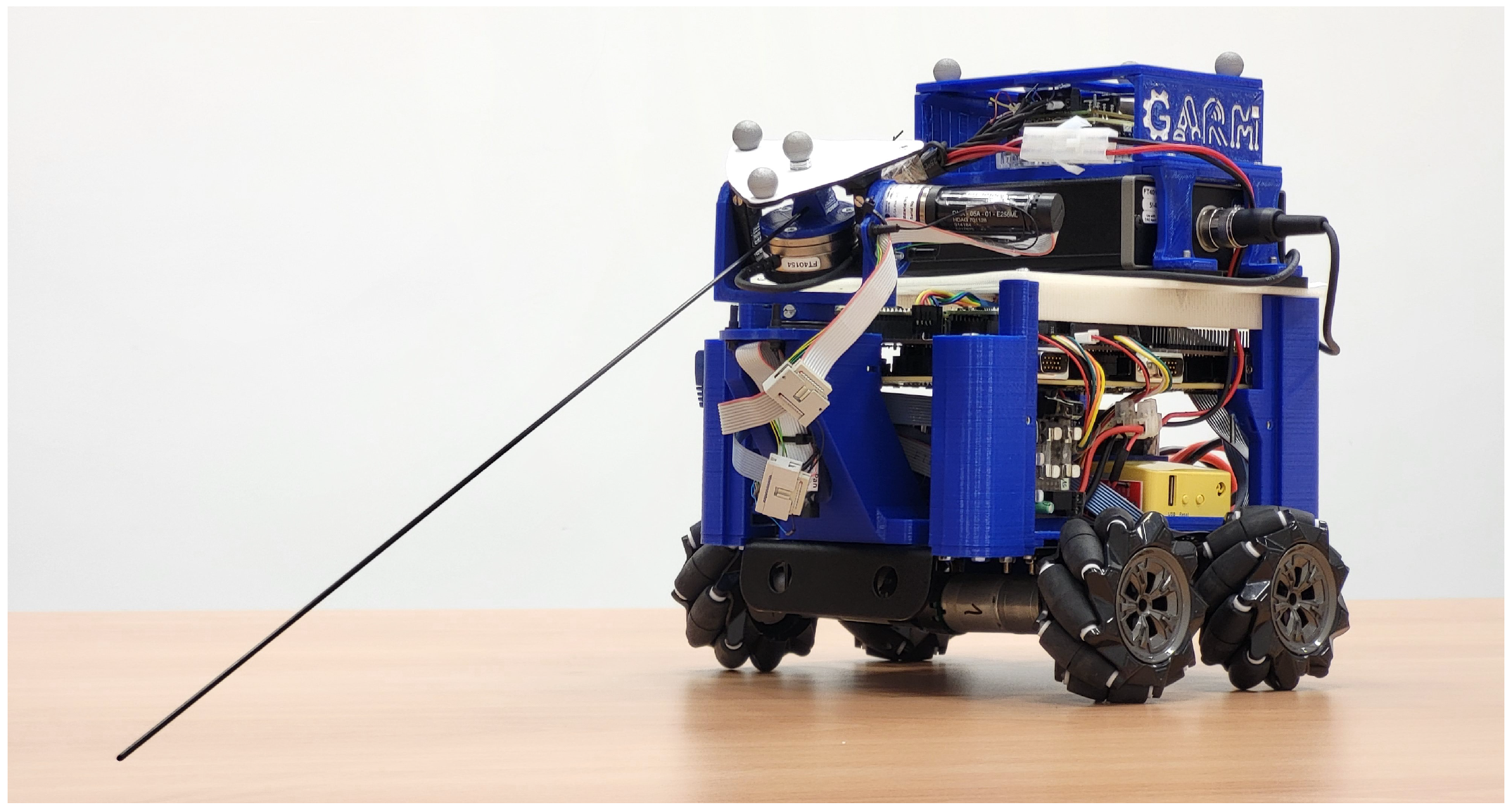
The $MRHS$ is shown in Figure 1. The $HSA$, which is mounted at the front of the $MWMR$, consists of a robotic subsystem that works as an active haptic system. Its design has been developed by our group in previous works [30,31], where it has been used as a tactile sensor to detect objects that are in its surroundings. It is mainly composed of a lightweight, slender carbon-fibre rod (the antenna) attached to one of its ends to a six-axis force–torque ($FT$) sensor ATI FTD-MINI40. In turn, the $FT$ sensor is fixed to a structure moved by two Harmonic Drive direct current ($DC$) mini-servo actuator PMA-5A motor sets that include zero backlash 1:50 reduction gears and incremental encoders.

Furthermore, carrying the $HSA$, there is the $MWMR$. It is composed of various subsystems. Firstly, the $MWMR$ platform consists of an aluminium chassis equipped with four $DC$ motors with incremental encoders and 1:75 reduction gears driving four 38 mm radius Mecanum wheels (also known as Swedish wheels, with rollers at ${45}^{\circ }$). The motors operate within ±9 V. Each encoder has a resolution of 4 pulses per turn of the motor axle, corresponding to 300 pulses per turn of the omni wheel. This setup achieves an accuracy of $\pm 1.2^{\circ }$ in measuring the wheel angular position.

The $MWMR$ also equips a National Instruments Field-Programmable Gate Array ($FPGA$) CompactRIO control board (sbRIO-9631). This board communicates with a host computer via a $Wifi$ Router, reads sensor measurements (motor encoders and the force–torque sensor from the $HSA$) and controls all the motors of the robot, including the $HSA$ and $MWMR$, using Maxon ESCON Module $24/2$ servo controller boards. These controller boards manage the inner current loops of the motors. The entire system is powered by two 3500 mAh, 3-cell (11.1 V) $LiPo$ batteries connected in series, delivering a nominal 22.2 V.

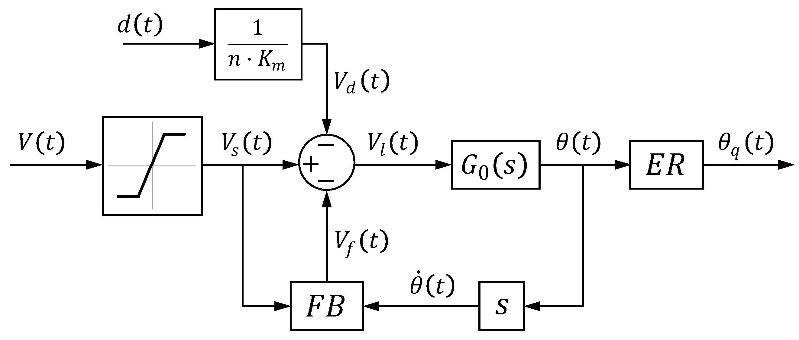
In this work, we will focus on the modelling and control of the $MWMR$. More details about this setup can be found in [12].

4. MWMR Model

The dynamic model of our mobile robot is developed in this section. First, a model of the system considering input disturbances is obtained. Then, the robot parameters identified in [12] are provided. Finally, the complete dynamic model of the $MWMR$ including nonlinearities is given.

4.1. Analytical Model

Figure 2 schematises the system in which the $MWMR$ displaces along the X axis, which has an $\alpha$ inclination slope. The robot mass is M and moves forward due to the applied force $F_a\left(t\right)$. Some assumptions are made: (1) the robot displaces due to the motor torques applied to the wheels by their respective motors, (2) perfect grip between the wheels and the ground is assumed, so no sliding nor skipping is considered, and (3) the drag force and rolling resistance are considered negligible.

Thus, the dynamics of the system are expressed as:

$$F_a\left(t\right)-M·g·sin\left(\alpha \right)=M·\ddot{x}\left(t\right)$$

(1)

where g is the gravity constant. The applied force $F_a\left(t\right)$ is the sum of the forces generated by the torques ${\mathrm{\Gamma }}_a^i\left(t\right)$ applied by each motor i through its wheel i:

$$F_a\left(t\right)=\frac{{\sum }_{i=1}^4{\mathrm{\Gamma }}_a^i\left(t\right)}{R}$$

(2)

where i denotes each motor/wheel as $i=1$ (Front-Left), $i=2$ (Front-Right), $i=3$ (Back-Left) and $i=4$ (Back-Right), and R is the radius of the wheels.

The applied torque i can be obtained from the dynamic equation of motor i:

$${\mathrm{\Gamma }}_a^i\left(t\right)={\mathrm{\Gamma }}_m^i\left(t\right)-J_m^i·{\ddot{\theta }}^i\left(t\right)-{\nu }^i·{\dot{\theta }}^i\left(t\right)-{\mathrm{\Gamma }}_f^i\left(t\right)$$

(3)

where ${\mathrm{\Gamma }}_m^i\left(t\right)$ is the motor torque, ${\theta }^i\left(t\right)$ the angular position of the motor and the corresponding wheel, $J_m^i$ and ${\nu }^i$ are the inertia and viscous friction of the motor, respectively, and ${\mathrm{\Gamma }}_f^i\left(t\right)$ is the nonlinear friction term. The motor torque ${\mathrm{\Gamma }}_m^i\left(t\right)$ is obtained by:

$${\mathrm{\Gamma }}_m^i\left(t\right)=n·K_m^i·V^i\left(t\right)$$

(4)

where n is the motor’s reduction gear ratio, $K_m^i$ is the electromechanical constant of the motor servo amplifier system and $V^i\left(t\right)$ is the motor input voltage. $V^i\left(t\right)$ is the control variable of the system, introduced to the servo amplifier to regulate the amount of current supplied to the motor. Therefore, a combination of the motor and the servo amplifier dynamics can be considered, obtaining a constant relation $K_m^i$ between the motor torque and input voltage [12].

As perfect grip between the wheels and the ground is considered, it can be assumed that the displacement of the robot along the X direction requires all the motors turning the same angle, ${\theta }^i\left(t\right)=\theta \left(t\right)$, $\forall i$. Thus, all four motors provide the same amount of torque, ${\mathrm{\Gamma }}_m^i\left(t\right)={\mathrm{\Gamma }}_m\left(t\right)$, $\forall i$. Moreover, the wheels are driven by the same type of motors and amplifiers, allowing for the assumption of homogeneity in physical parameters, which implies that ${\mathrm{\Gamma }}_a^i\left(t\right)={\mathrm{\Gamma }}_a\left(t\right)$, $\forall i$, and, then, Equation (2) can be approximated by

$$F_a\left(t\right)\approx 4·\frac{{\mathrm{\Gamma }}_a\left(t\right)}{R}$$

(5)

and Equation (3) can be rewritten considering (4) as:

$${\mathrm{\Gamma }}_a\left(t\right)=n·K_m·V\left(t\right)-J_m·\ddot{\theta }\left(t\right)-\nu ·\dot{\theta }\left(t\right)-{\mathrm{\Gamma }}_f\left(t\right)$$

(6)

The combination of (1), (5) and (6) and the relation between the angle of the motor-wheel and its relative displacement in X, that is, $x\left(t\right)=\theta \left(t\right)·R$, leads to the general dynamic equation of the system:

$$n·K_m·V\left(t\right)=\left(J_m+\frac{M·R^2}{4}\right)·\ddot{\theta }\left(t\right)+\nu ·\dot{\theta }\left(t\right)+{\mathrm{\Gamma }}_f\left(t\right)+\frac{R}{4}·M·g·sin\left(\alpha \right)$$

(7)

The last addend of (7) represents the disturbance effect caused by the slope that the robot is supposed to face, which henceforth will be denoted as d:

$$d=\frac{R}{4}·M·g·sin\left(\alpha \right)$$

(8)

A transfer function can be obtained between $V\left(t\right)$ and $\theta \left(t\right)$ by removing ${\mathrm{\Gamma }}_f\left(t\right)$ and d from (7)—because they are considered as disturbances—and taking Laplace transforms:

$$\widehat{G}\left(s\right)=\frac{\theta \left(s\right)}{V\left(s\right)}=\frac{\frac{n·K_m}{J}}{s^2+\frac{\nu }{J}·s}=\frac{A}{s·(s+B)}$$

(9)

being $J=J_0=J_m+\frac{M·R^2}{4}$, and A, B the terms that comprehend the motor parameters.

4.2. Identification Method of the Parameters of the $MWMR$

Motor parameters A and B of (9) are identified through a process in which different voltages $V\left(t\right)$ are applied and data $\dot{\theta }\left(t\right)$ are registered by numerically differentiating the measurement $\theta \left(t\right)$ of the encoder. Then, $\dot{\theta }\left(s\right)/V\left(s\right)=A/(s+B)$, and these parameters are determined by using well-known relations of first-order systems [32]:

$$B=\frac{3}{t_s},A=P_m·B$$

(10)

being $t_s$ the settling time and $P_m$ the system gain (the relation between the applied voltage and the angular velocity reached in a steady state, ${\dot{\theta }}_s$). Both $t_s$ and $P_m$ are easily obtained from that experimental data.

The electromechanical constant of the motor servo amplifier system $K_m$ is determined from the data provided by the motor manufacturer, being $K_m=1.74·{10}^{-3}$ Nm/V.

During the identification process, the time delay L appears. It is caused by a combination of the reduction gears backlash and the speeds of the control board. Then, the linear dynamics (9) are modified to the transfer function

$$G\left(s\right)=\widehat{G}\left(s\right)·e^{-L·s}=\frac{A}{s·(s+B)}·e^{-L·s}$$

(11)

Also during the identification process, some nonlinearities appear and need to be identified. The nonlinear friction term ${\mathrm{\Gamma }}_f\left(t\right)$ is a torque that brakes the motor when applying low-input voltages to the motor, causing it to get stuck (motor dead-zone), and when running the motor at non-zero speed, avoiding the motor reaching the desirable angular velocity (Coulomb friction). Because the torque is proportional to the voltage, the friction model ${\mathrm{\Gamma }}_f\left(t\right)$ can be expressed in terms of its equivalent voltage $V_f\left(t\right)$ by means of the following piecewise function:

$$V_f\left(t\right)=\left\{\begin{array}{cc}{V}_f^K·sign\left(\dot{\theta }\left(t\right)\right),\hfill & |\dot{\theta }\left(t\right)|\ne 0\hfill \\ V_f^S·sign\left(V\left(t\right)\right),\hfill & |\dot{\theta }\left(t\right)|=0\hfill & and\hfill & \left|V\left(t\right)\right|>V_f^S\hfill \\ V\left(t\right),\hfill & |\dot{\theta }\left(t\right)|=0\hfill & and\hfill & \left|V\left(t\right)\right|\le V_f^S\hfill \end{array}\right.$$

(12)

being $V_f^S$ the stiction break-away equivalent voltage, $V_f^K$ the kinetic friction equivalent voltage and $V_f^S>V_f^K$.

Other nonlinear phenomena that must be considered are the saturation and encoder resolution. Experiments have been performed to figure out the real motor saturation value, obtaining $V_{sat}=8.7$ V, which is slightly different to the value of 9 V given by the manufacturer. Regarding the measuring resolution, one pulse of the equipped encoders is equal to $1.2^{\circ }$ in the wheel angle. This is such a significant jump when controlling the position of the wheels and needs to be replicated in the model to assess the impact of this quantisation in the control system. Hence, the signal $\theta \left(t\right)$ will be truncated yielding the signal ${\theta }_q\left(t\right)$.

More details of this identification procedure can be found in [12].

4.3. Complete Model of the System

Figure 3 represents a block diagram of the full motor model. First, the input signal $V\left(t\right)$ is limited by means of a saturation block to a maximum absolute value defined by $V_{sat}$, delivering the voltage signal $V_s\left(t\right)$. After that, the friction equivalent voltage $V_f\left(t\right)$ is generated by (12) in the friction block FB $(V,\dot{\theta })$. Also, the disturbance effect of the slope (8) is calculated in terms of voltage $V_d\left(t\right)$ through n and $K_m$. Subtracting $V_f\left(t\right)$ and $V_d\left(t\right)$ from $V_s\left(t\right)$ gives $V_l\left(t\right)$, which is the torque equivalent voltage moving the undisturbed linear part of the system $G_0\left(s\right)$, represented by the transfer function (11), whose output is $\theta \left(t\right)$. Later, this signal is differentiated to obtain the velocity $\dot{\theta }\left(t\right)$. Finally, the encoder resolution is replicated in the block ER by truncating the signal $\theta \left(t\right)$, yielding ${\theta }_q\left(t\right)$.

The mean values of the parameters identified obtained from [12] are presented in

Table 1. Identification results.

${\mathit{A}}_0$	${\mathit{B}}_0$	${\mathit{L}}_0$ (s)	${\mathit{V}}_{\mathit{f}}^{\mathit{S}}$ (V)	${\mathit{V}}_{\mathit{f}}^{\mathit{K}}$ (V)
1631.32	19.97	0.0539	0.85	0.2898

. With those mean values, the corresponding nominal transfer function $G_0\left(s\right)$ is defined as:

$$G_0\left(s\right)=\frac{\theta \left(s\right)}{V_l\left(s\right)}=\frac{A_0}{s·(s+B_0)}·e^{-L_0·s}=\frac{1631}{s·(s+19.97)}·e^{-0.0539·s}$$

(13)

5. Proposed Control System

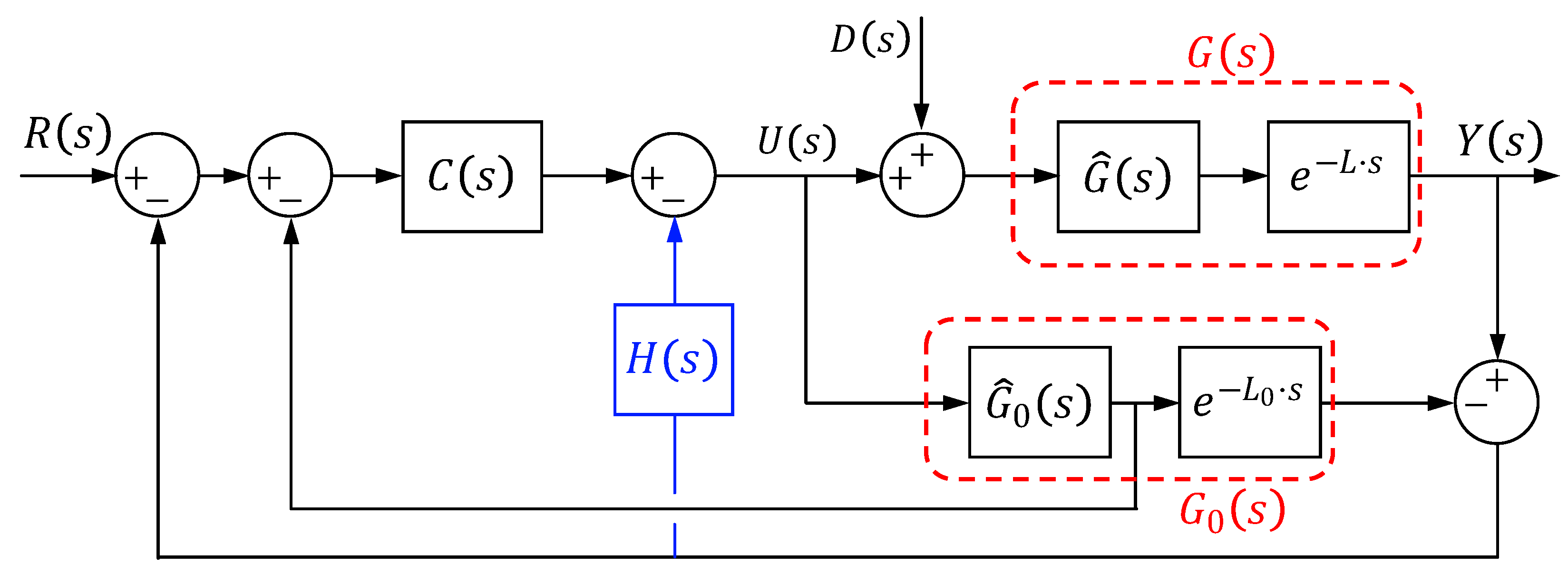
We propose to use the control scheme developed originally in [29] for a stable second-order plus time delay process. This control scheme is a modification of the $SP$, which is denoted $SP$-H. It is based on adding a feedback of the difference between the process output and the nominal model output to the standard $SP$, as it is shown in Figure 4. Then, we will first provide a brief description of the standard $SP$ and, after, we will develop our new controller. In this section, we will neglect the nonlinear behaviour of the motors, i.e., Coulomb friction and saturation, because we assume that their effects are approximately removed by a friction compensator and an antiwindup system, as it was mentioned in the Introduction and in [12]. Then, this section focuses on developing and comparing controllers for linear systems.

5.1. Standard $SP$ Scheme

The standard $SP$ control scheme is represented by the black lines and boxes shown in Figure 4. In this figure, $G\left(s\right)$ is the process to be controlled, which is composed of a rational part, $\widehat{G}\left(s\right)$, and a term $e^{-L·s}$ corresponding to the time delay L. $G_0\left(s\right)$ represents the nominal model of $G\left(s\right)$, which is composed of a nominal rational part, ${\widehat{G}}_0\left(s\right)$, and a term $e^{-L_0·s}$ corresponding to the nominal time delay $L_0$. $R\left(s\right)$ is the input (reference) signal, $C\left(s\right)$ is the main controller, $U\left(s\right)$ is the control signal, $Y\left(s\right)$ is the plant output signal and $D\left(s\right)$ is the load disturbance signal. It is not difficult to obtain the transfer functions between the output $Y\left(s\right)$ and the reference $R\left(s\right)$, and between the output $Y\left(s\right)$ and the disturbance $D\left(s\right)$, which are, respectively,

$$T_r\left(s\right)=\frac{Y\left(s\right)}{R\left(s\right)}=\frac{C\left(s\right)·\widehat{G}\left(s\right)·e^{-L·s}}{1+C\left(s\right)·\left({\widehat{G}}_0\left(s\right)+\widehat{G}\left(s\right)·e^{-L·s}-{\widehat{G}}_0\left(s\right)·e^{-L_0·s}\right)}$$

(14)

$$T_d\left(s\right)=\frac{Y\left(s\right)}{D\left(s\right)}=\frac{1+C\left(s\right)·{\widehat{G}}_0\left(s\right)·\left(1-e^{-L_0·s}\right)}{1+C\left(s\right)·\left({\widehat{G}}_0\left(s\right)+\widehat{G}\left(s\right)·e^{-L·s}-{\widehat{G}}_0\left(s\right)·e^{-L_0·s}\right)}·\widehat{G}\left(s\right)·e^{-L·s}$$

(15)

In this scheme, two predictors with their respective closed loops are implemented. The first one implements the nominal dynamics of the process $G_0\left(s\right)$ and its predicted output is subtracted to the real output yielding the signal that is fed back into this loop. This loop is inactive if the real process coincides with the model and there is not a disturbance. Otherwise, this loop is active, being in charge of rejecting the output errors caused by these two issues. The second predictor implements the model without its delay ${\widehat{G}}_0\left(s\right)$ and predicts the value of the process output $L_0$ s in advance. This prediction is used to close a loop in which the delay of the process is removed, which facilitates the design of the controller $C\left(s\right)$. This loop is essentially in charge of making the process track the reference.

In the case of the nominal process, i.e., $G\left(s\right)=G_0\left(s\right)$, the previous transfer functions become

$$T_r\left(s\right)=\frac{Y\left(s\right)}{R\left(s\right)}=\frac{C\left(s\right)·{\widehat{G}}_0\left(s\right)·e^{-L_0·s}}{1+C\left(s\right)·{\widehat{G}}_0\left(s\right)}$$

(16)

$$T_d\left(s\right)=\frac{Y\left(s\right)}{D\left(s\right)}=\frac{1+C\left(s\right)·{\widehat{G}}_0\left(s\right)·\left(1-e^{-L_0·s}\right)}{1+C\left(s\right)·{\widehat{G}}_0\left(s\right)}·{\widehat{G}}_0\left(s\right)·e^{-L_0·s}$$

(17)

Note that the delay has disappeared from the denominator of both transfer functions, as it was advanced in the previous paragraph. Then, the characteristic equation of this closed-loop system becomes rational and it is possible to apply standard linear control design techniques to achieve the desired closed-loop specifications.

The analysis of the steady-state performance of the $SP$ in the case of the nominal process is carried out using (16) and (17), and the final value theorem, e.g., [32]:

1.

Step reference.

(a)

In the case that ${\widehat{G}}_0\left(s\right)$ is not integrating, i.e., it does not have a pole located at the origin of the complex plane, the steady-state error of its step response is non-zero if $C\left(s\right)$ is not integrating (e.g., a $PD$ controller) and is zero if $C\left(s\right)$ is integrating (e.g., a $PID$ controller).

(b)

In the case that ${\widehat{G}}_0\left(s\right)$ is integrating, i.e., it has a pole located at the origin of the complex plane, the steady-state error of its step response is zero in both cases: integrating and not integrating $C\left(s\right)$.

2.

Step disturbance rejection.

(a)

In the case that ${\widehat{G}}_0\left(s\right)$ is not integrating, a step disturbance produces a non-zero steady-state error in the output if $C\left(s\right)$ is not integrating and a zero steady-state error if $C\left(s\right)$ is integrating.

(b)

In the case that ${\widehat{G}}_0\left(s\right)$ is integrating, a step disturbance produces a non-zero steady-state error in both cases: integrating and not integrating $C\left(s\right)$.

The transfer functions of our motors have the form (13). Then, they are $IPTD$ processes. Because the terrain slope effect is modelled as a step disturbance of unknown amplitude d given by (8)—the angle $\alpha$ of the slope is unknown—the previous analysis yields (see Case 2b) that the standard $SP$ controller is unable to obtain a zero steady-state error in robot positioning. A modification of the basic $SP$ scheme is therefore required to overcome this drawback.

5.2. Modified $SP$ Scheme: The $SP$-H Scheme

This modification utilises the existing prediction of the time delay compensator and decouples the set-point response from the disturbance response. The set-point response and the disturbance response of the closed-loop system are adjusted by two controllers. Figure 4 shows this new $SP$ scheme that is composed of the standard $SP$ scheme with its controller $C\left(s\right)$ plus a new feedback loop that includes the second controller $H\left(s\right)$, highlighted in blue in the figure.

Simplifying the complete block diagram of Figure 4, we obtain now that

$$Y\left(s\right)=T_r^{\prime }\left(s\right)·R\left(s\right)+T_d^{\prime }\left(s\right)·D\left(s\right)$$

(18)

where

$$T_r^{\prime }\left(s\right)=\frac{Y\left(s\right)}{R\left(s\right)}=\frac{C\left(s\right)·\widehat{G}\left(s\right)·e^{-L·s}}{1+C\left(s\right)·{\widehat{G}}_0\left(s\right)+\left(C\left(s\right)+H\left(s\right)\right)·\left(\widehat{G}\left(s\right)·e^{-L·s}-{\widehat{G}}_0\left(s\right)·e^{-L_0·s}\right)}$$

(19)

$$T_d^{\prime }\left(s\right)=\frac{Y\left(s\right)}{D\left(s\right)}=\frac{1+{\widehat{G}}_0\left(s\right)·\left(C\left(s\right)-\left(C\left(s\right)+H\left(s\right)\right)·e^{-L_0·s}\right)}{1+C\left(s\right)·{\widehat{G}}_0\left(s\right)+\left(C\left(s\right)+H\left(s\right)\right)·\left(\widehat{G}\left(s\right)·e^{-L·s}-{\widehat{G}}_0\left(s\right)·e^{-L_0·s}\right)}·\widehat{G}\left(s\right)·e^{-L·s}$$

(20)

Note that transfer functions (14) and (15) are, respectively, obtained from (19) and (20) by just making $H\left(s\right)=0$.

In the case of the nominal process, i.e., $G\left(s\right)=G_0\left(s\right)$, the transfer functions of (18) are

$$T_r^{\prime }\left(s\right)=\frac{C\left(s\right)·{\widehat{G}}_0\left(s\right)·e^{-L_0·s}}{1+C\left(s\right)·{\widehat{G}}_0\left(s\right)}$$

(21)

$$T_d^{\prime }\left(s\right)=\frac{1+{\widehat{G}}_0\left(s\right)·\left(C\left(s\right)-\left(H\left(s\right)+C\left(s\right)\right)·e^{-L_0·s}\right)}{1+C\left(s\right)·{\widehat{G}}_0\left(s\right)}·{\widehat{G}}_0\left(s\right)·e^{-L_0·s}$$

(22)

In the case of the nominal process, transfer function (21) shows that the set-point tracking performance depends on $C\left(s\right)$ and it does not depend on $H\left(s\right)$. However, the transfer function (22) shows that the disturbance rejection performance depends on both $C\left(s\right)$ and $H\left(s\right)$.

From now on, we will consider that $y\left(t\right)$ is the motor angle $\theta \left(t\right)$, and the process input $u\left(t\right)$ is the motor voltage $V_l\left(t\right)$ that moves the undisturbed linear part of the system, and $G\left(s\right)=G_0\left(s\right)$ is given by (13). Moreover, because the disturbance is a step, $D\left(s\right)=d/s$.

5.3. Stability Issues

In the case of the nominal process, the closed-loop stability is defined by the denominator of (21) and (22). Because it is a polynomial in s, the stability is defined by a proper design of $C\left(s\right)$, which can be performed by any method to design controllers for linear time-invariant systems.

In the case of a mismatch between the model and the real process, the stability robustness can be studied using the following condition in the frequency domain, which was derived in [29]:

$$\mathrm{\Phi }\left(\omega \right)>\left|\Delta (j·\omega )\right|$$

(23)

where $\Delta (j·\omega )$ is the relative mismatch:

$$\Delta (j·\omega )=\frac{\widehat{G}(j·\omega )·e^{-j·L·\omega }-{\widehat{G}}_0(j·\omega )·e^{-j·L_0·\omega }}{{\widehat{G}}_0(j·\omega )·e^{-j·L_0·\omega }}$$

(24)

and

$$\mathrm{\Phi }\left(\omega \right)=\left|\frac{C(j·\omega )·{\widehat{G}}_0(j·\omega )+1}{\left(C(j·\omega )+H(j·\omega )\right)·{\widehat{G}}_0(j·\omega )}\right|$$

(25)

5.4. Design of $C\left(s\right)$

Because the integrating term of our $IPTD$ process guarantees the zero steady-state error to a step command, we will design a $PD$ controller

$$C\left(s\right)=K_p+K_d·s$$

(26)

in order to obtain the desired dynamics of the closed-loop system. Because $\widehat{G}\left(s\right)$ is a second-order system, according to the common denominator of (21) and (22), $PD$ (26) will allow us to freely allocate the two poles of the closed-loop system.

The characteristic equation of the closed-loop system (21), (22) is

$$1+\frac{A_0}{s·\left(s+B_0\right)}·\left(K_p+K_d·s\right)=0\Rightarrow s^2+\left(B_0+A_0·K_d\right)·s+A_0·K_p=0$$

(27)

Because the right side of (27) is a second-order equation, the closed-loop system has two poles $p_1$, $p_2$ that can be arbitrarily placed by tuning $K_p$ and $K_d$. Equating coefficients of the same powers of s between (27) and $\left(s-p_1\right)·\left(s-p_2\right)=s^2-\left(p_1+p_2\right)·s+p_1·p_2$ yields the tuning rules

$$K_p=\frac{p_1·p_2}{A_0},K_d=-\frac{p_1+p_2+B_0}{A_0}$$

(28)

We will show that, in our mobile robot, we obtain satisfactory results designing a critically damped system with the double pole placed in $-B_0/2$. In this case, $K_d$ becomes 0 and we use a P controller of the form $C\left(s\right)=\frac{B_0^2}{4·A_0}$.

5.5. Design the Compensator $H\left(s\right)$

As previously mentioned, several modified $SPs$ with different structures have been proposed in the literature for $IPTD$ processes to remove the steady-state error produced by a constant load disturbance. Some of them reduce the steady-state disturbance error and others completely eliminate that error. We seek in this subsection to design a modified $SP$ that completely eliminates the steady-state disturbance error and, moreover, reduces the transient disturbance error more effectively than other methods. This is based on a proper design of $H\left(s\right)$.

Substituting $G\left(s\right)$ by (13) and $C\left(s\right)$ by (26) in (22) gives that

$$T_d^{\prime }\left(s\right)=\frac{s·(s+B_0)+A_0·\left[K_p+K_d·s-\left(H\left(s\right)+K_p+K_d·s\right)·e^{-L_0·s}\right]}{s^2+\left(B_0+A_0·K_d\right)·s+A_0·K_p}·\frac{A_0}{s·(s+B_0)}·e^{-L_0·s}$$

(29)

The steady-state error of $y\left(t\right)$ in response to a step load distance $d\left(t\right)$ is given by the final value theorem, e.g., [32]:

$$e_{pd}=\underset{t\to \infty }{lim}e\left(t\right)=\underset{s\to 0}{lim}s·T_d^{\prime }\left(s\right)·\frac{d}{s}$$

(30)

Then, in order to make $e_{pd}=0$, the following are necessary:

1.

The numerator of $T_d^{\prime }\left(s\right)$ must be 0 at $s=0$ in order to have a finite $e_{pd}$. Then,

$${\left.\left(s·(s+B_0)+A_0·\left[K_p+K_d·s-\left(H\left(s\right)+K_p+K_d·s\right)·e^{-L_0·s}\right]\right)\right|}_0=0\Rightarrow H\left(0\right)=0$$

(31)

2.

The derivative of the numerator of $T_d^{\prime }\left(s\right)$ with respect to s must be 0 at $s=0$ in order to make $e_{pd}$ equal to zero. Then,

$$\begin{array}{ccc}\hfill {\left.\frac{d\left(s·(s+B_0)+A_0·\left[K_p+K_d·s-\left(H\left(s\right)+K_p+K_d·s\right)·e^{-L_0·s}\right]\right)}{ds}\right|}_0& =& 0\Rightarrow \hfill \end{array}$$

(32)

$$\begin{array}{ccc}\hfill {\left.\frac{dH\left(s\right)}{ds}\right|}_{s=0}=K_p·L_0+\frac{B_0}{A_0}& & \hfill \end{array}$$

(33)

The first condition implies that $H\left(s\right)$ must have a zero (of any multiplicity) at the origin. Then, $H\left(s\right)$ must have the form

$$H\left(s\right)=\frac{s^m·H_n\left(s\right)}{H_d\left(s\right)}$$

(34)

where $H_n\left(0\right)\ne 0$ and $H_d\left(0\right)=1$. The second condition imposes that

$${\left.\frac{dH\left(s\right)}{ds}\right|}_{s=0}=\underset{s\to 0}{lim}\frac{m·s^{m-1}·H_n\left(s\right)}{H_d\left(s\right)}=K_p·L_0+\frac{B_0}{A_0}$$

(35)

which can only be satisfied if $m=1$. Then, we propose the simplest $H\left(s\right)$ that verifies the previous conditions:

$$H\left(s\right)=\frac{\left(K_p·L_0+\frac{B_0}{A_0}\right)·s}{1+\lambda ·s},\lambda >0$$

(36)

Note that the closed-loop steady-state error and $H\left(s\right)$ do not depend on the derivative gain $K_d$ of $C\left(s\right)$, only on the proportional gain $K_p$.

Then, a compensator $H\left(s\right)$ of the form (36) improves the disturbance rejection capabilities of the system without affecting the nominal set-point response.

6. Comparison with Other SP Modifications

In this section, the performance of the proposed scheme is evaluated during the set-point tracking and load disturbance by comparing it with well-known modified $SP$ schemes. The simulations of four reputed modified $SP$ schemes are carried out, reported by Smith [16] (the original $SP$); Stojic, Matijevic [33]; Normey-Rico, Julio and Camacho, Eduardo [34]; and Espín, Jorge et al. [28], in addition to our proposed scheme. The first three schemes are linear controllers, while the fourth one is a nonlinear scheme based on sliding-mode control. We apply these different control structures to the nominal process (13) facing a step input reference of $\pi$ radians and a disturbance applied at 2 s. Two types of disturbances are simulated: a step disturbance of amplitude 2 and a unitary slope ramp disturbance. The linear schemes use the same $C\left(s\right)$; meanwhile, the nonlinear controller is set up so that the system performs equivalent to the linear control schemes facing the step input reference.

As in the previous section, we will neglect the nonlinear behaviours of the motors because we will assume that they are compensated. Then, the linear system (13) will be used in the comparison. The parameters of $C\left(s\right)$ and $H\left(s\right)$ are set leading to the following expressions:

$$C\left(s\right)=0.061096;H\left(s\right)=\frac{0.01529·s}{0.05·s+1}$$

(37)

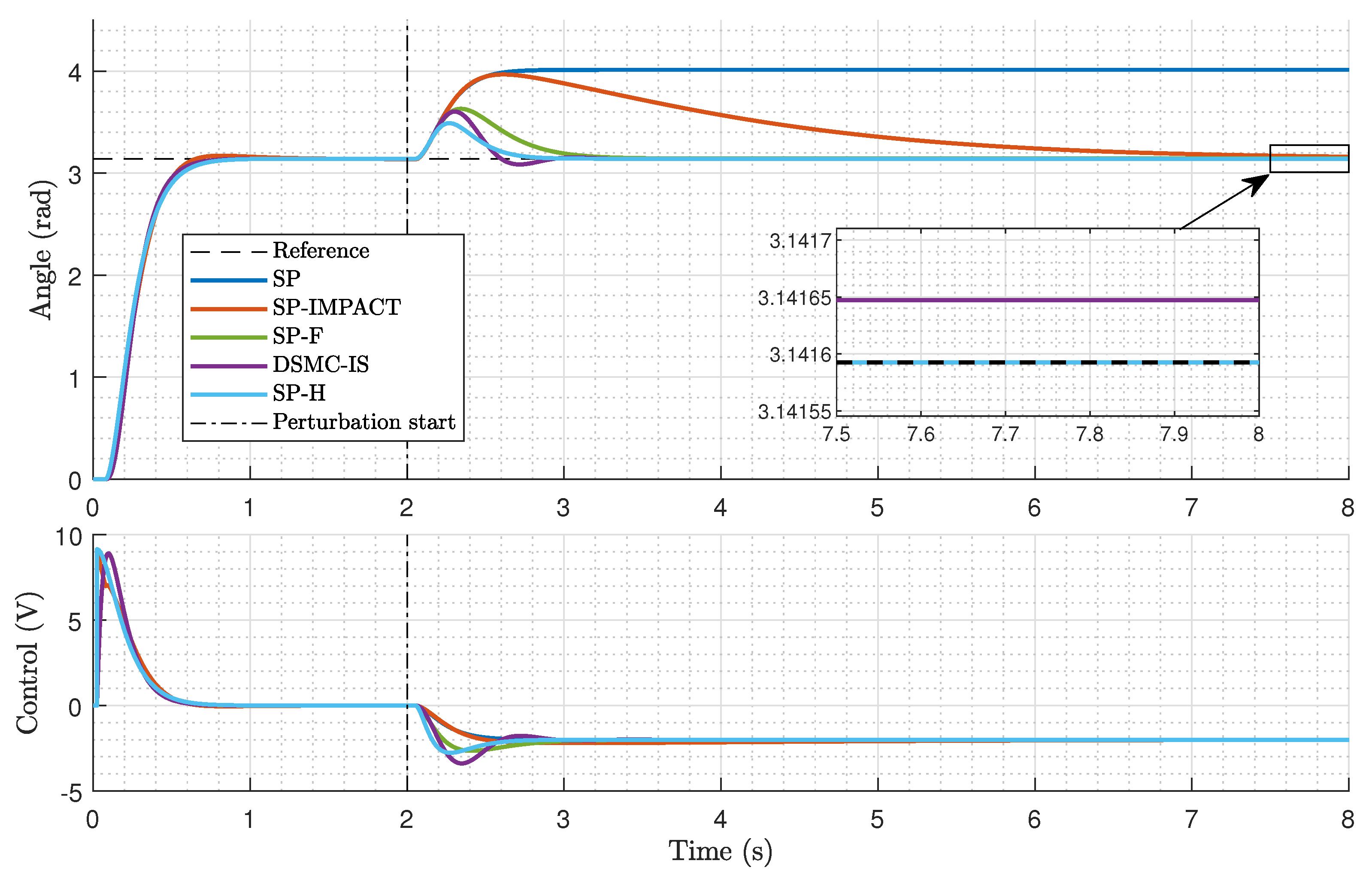
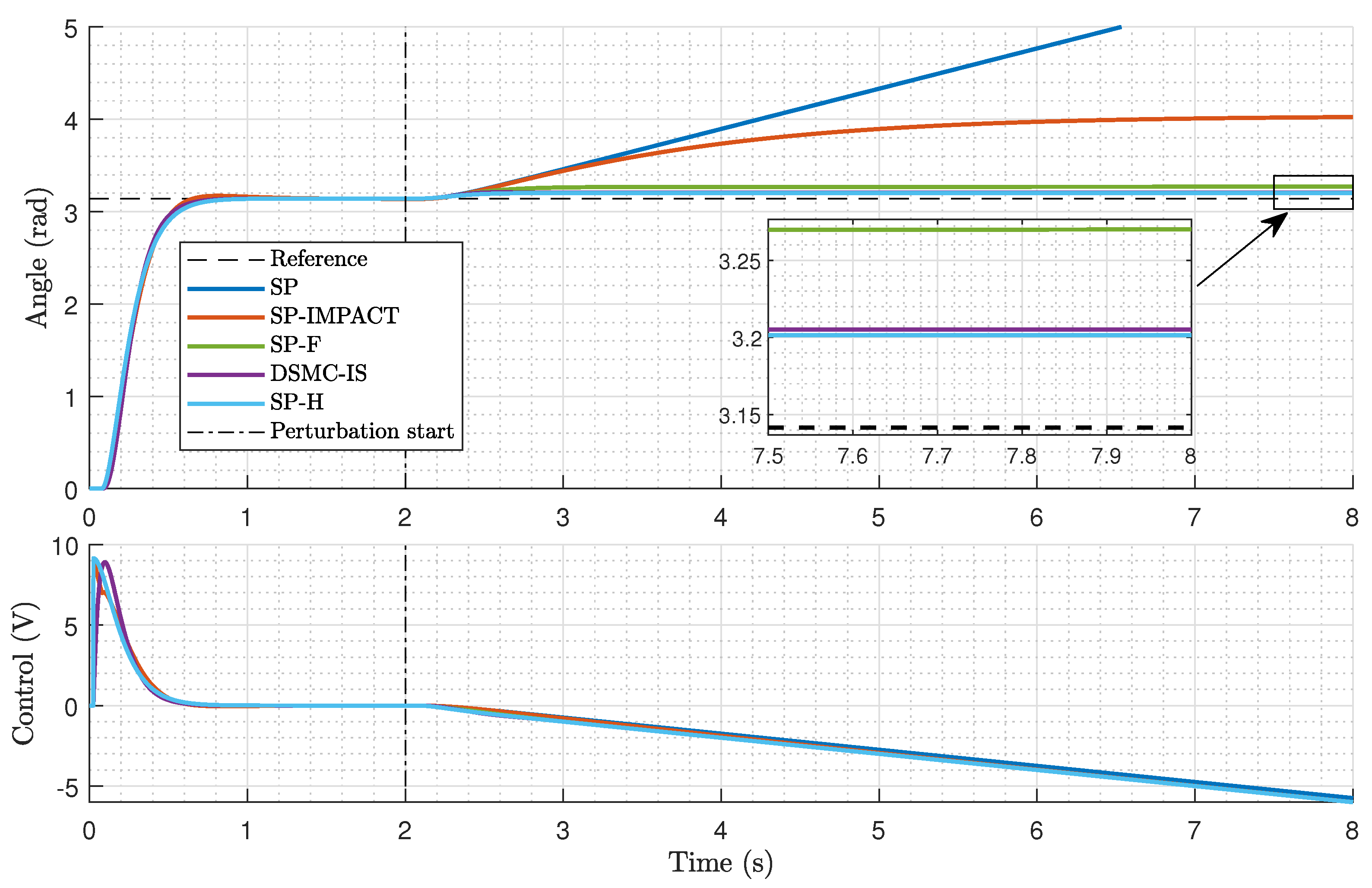
The process outputs using the before controllers and facing a step disturbance are illustrated in Figure 5. All of them provide the same response to a set-point change—then they may be considered as equivalent—but they show differences in the external disturbance rejection, both in the transient and in the steady-state error. The original $SP$ does not have a block responsible for rejecting the disturbance. For this reason, it is unable to cancel a step disturbance in the process input. The other schemes have their own blocks responsible for eliminating the disturbance.

In [33], the proposed $SP$ (denoted as $SP$-$IMPACT$) has an observer estimator that enables absorbing any class of disturbance. The control part of the modified $SP$ contains five parameters, $K_v$, L, $K_r$, $T_0$ and n. Two of them are the plant parameters $K_v$ (gain) and L (time delay). The other three parameters, $K_r$, $T_0$ and n, are to be adjusted with respect to the prescribed set-point change transient speed and the disturbance transient response and to the desired robustness to mismatches in $K_v$ and L.

On the other hand, the filtered $SP$ (denoted as $SP$-F) introduced by [34] contains a block disturbance rejection represented by the filter $F_r\left(s\right)$, which is placed in the feedback of the control scheme. This filter is used to improve the robustness and the disturbance rejection capabilities of the system without affecting the nominal set-point response.

Also, the nonlinear control scheme presented by [28] (denoted as $DSMC$-$IS$), which is a combination of a modified $SP$ and a sliding-mode controller, is able to reject the disturbance by means of a $PD$ compensator placed in its inner loop. It considerably reduces the steady-state error compared to the previous schemes, but still is not zero, as detailed in Figure 5.

Our proposed modified Smith predictor $SP$-H involves only two controllers: the controller $C\left(s\right)$ used to follow the set-point changes (or trajectory tracking) and the compensator $H\left(s\right)$ used to improve the disturbance rejection. The simulations shown in Figure 5 illustrate that the $SP$-H provides the best disturbance rejection features, performing the best disturbance transient response of all and a zero steady-state error.

The process outputs using the before controllers and facing a unitary slope ramp disturbance are illustrated in Figure 6. In this case, all the schemes show a higher steady-state error due to the nature of the disturbance, but once again, the best result comes from our $SP$-H scheme, with the smallest steady-state error.

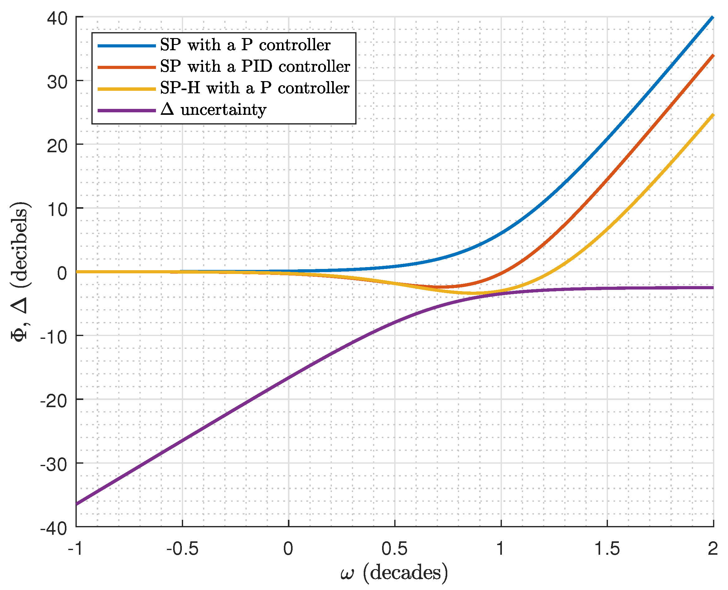
Finally, the robustness of our $SP$-H is compared to the robustness of the standard $SP$ by plotting in Figure 7 the respective $\mathrm{\Phi }\left(\omega \right)$ functions given by (25) ($H\left(s\right)$ is made zero in the case of the $SP$). Three controllers are compared: an $SP$ combined with a P controller, an $SP$ combined with the $PID$ controller designed in [12] and an $SP$-H with a P controller. All these controllers are tuned to have a closed-loop double pole in $p=-B_0/2\approx -10$ in order to make a fair comparison. This figure shows that the $SP$-H is the less robust control system, though it has a robustness similar to the $SP$ with a $PID$ in the range from 0 to 4 rad/s.

Because the payload M carried by the robot varies, the parameter that is most likely to change is J. Then, it is important to assess the robustness of the control systems in Figure 7 to this uncertainty. In this figure, $\Delta$ is plotted for $J=4·J_0$, which is the maximum expected inertia. It shows that, for this payload, the three control systems verify the robustness condition (23). Then, though the $SP$-H has the lowest robustness feature, it is sufficient for the working conditions foreseen for our robot.

7. Experimental Results

The comparison analysis of the previous section was carried out assuming a motor with linear dynamics. However, as it was previously stated, our motor has some nonlinearities such as Coulomb friction, actuator saturation and a low resolution of the encoders that degrade the controlled system performance. In the previous paper [12], these nonlinear effects were compensated by including in the control system a friction compensator and an antiwindup system. Moreover, the effect of a step input disturbance was reduced (though not removed) by using an integrating controller (a $PID$). Such a $PID$ produced (a) an undesired overshoot, which was removed, including a prefilter; (b) actuator saturation, for which the effect was reduced by the mentioned antiwindup system; and (c) a reduction in the relative stability of the closed-loop system (compare the $SP$ plots in Figure 7), which makes it prone to instability if the time delay or the carried payload change. Instead, our proposal keeps the friction compensator but, because it is able to completely eliminate the steady-state error at the output without needing to use an integrating controller, a simple P controller is used. This controller does not add additional zeros that may produce undesired overshoots, as the $PID$ does, and, unlike the $PID$, it does not have the integrating term that is responsible for the saturation phenomena in our motor. Then, because the prefilter and the antiwindup system were not needed, they were removed, and the control system is highly simplified.

Then, the experimental results are presented in this section that compare our new control system with the prior control scheme developed in [12]. The purpose of this comparison is to assess the previous assertions that our control system eliminates the steady-state error positioning while the prior control system does not, yields an approximately linear behaviour (as [12] does) and avoids overshoot and saturation (as [12] does), but it is a much simpler controller than [12]. The control schemes are implemented in the National Instruments control board of the robot through the LabView software and a few experiments are carried out.

7.1. Design of the Trajectory and Disturbance

The typical input signal references used to design the controllers are step signals. Nevertheless, it is a non-desirable reference in trajectory tracking because it introduces very high accelerations to the robot, causing unexpected robot behaviours, such as wheel slipping and trajectory deviation. Thus, a suitable fast input signal is designed with limited velocity and acceleration.

A Cartesian trajectory is designed for the robot to move along its longitudinal axis. It is set to displace 1 m with limited acceleration and speed. The input reference, which is expressed in time, is divided into three stages: a first stage with constant acceleration in which the robot accelerates until a determined speed; a second stage in which the robot displaces, maintaining speed; and a third stage in which the robot decelerates until it stops at the desired position. Finally, a steady-state stage is added at the end of the trajectory, where the robot remains in its final position. The maximum acceleration and speed values are carefully chosen to ensure that the robot maintains good ground adherence and avoids overloading the motors. Thus, the acceleration is set to 200 mm/s² and the maximum speed to 100 mm/s.

The input reference to the control scheme is the angular position of the motors. Hence, the designed trajectory (in X) needs to be transformed into the motor angular position $\theta \left(t\right)$ through $x\left(t\right)=R·\theta \left(t\right)$, where the radius of the wheel is $R=38$ mm. Also, the motor angles, which are the encoder measurements, can be transformed into the robot position in X through the same expression assuming the perfect grip of the wheels.

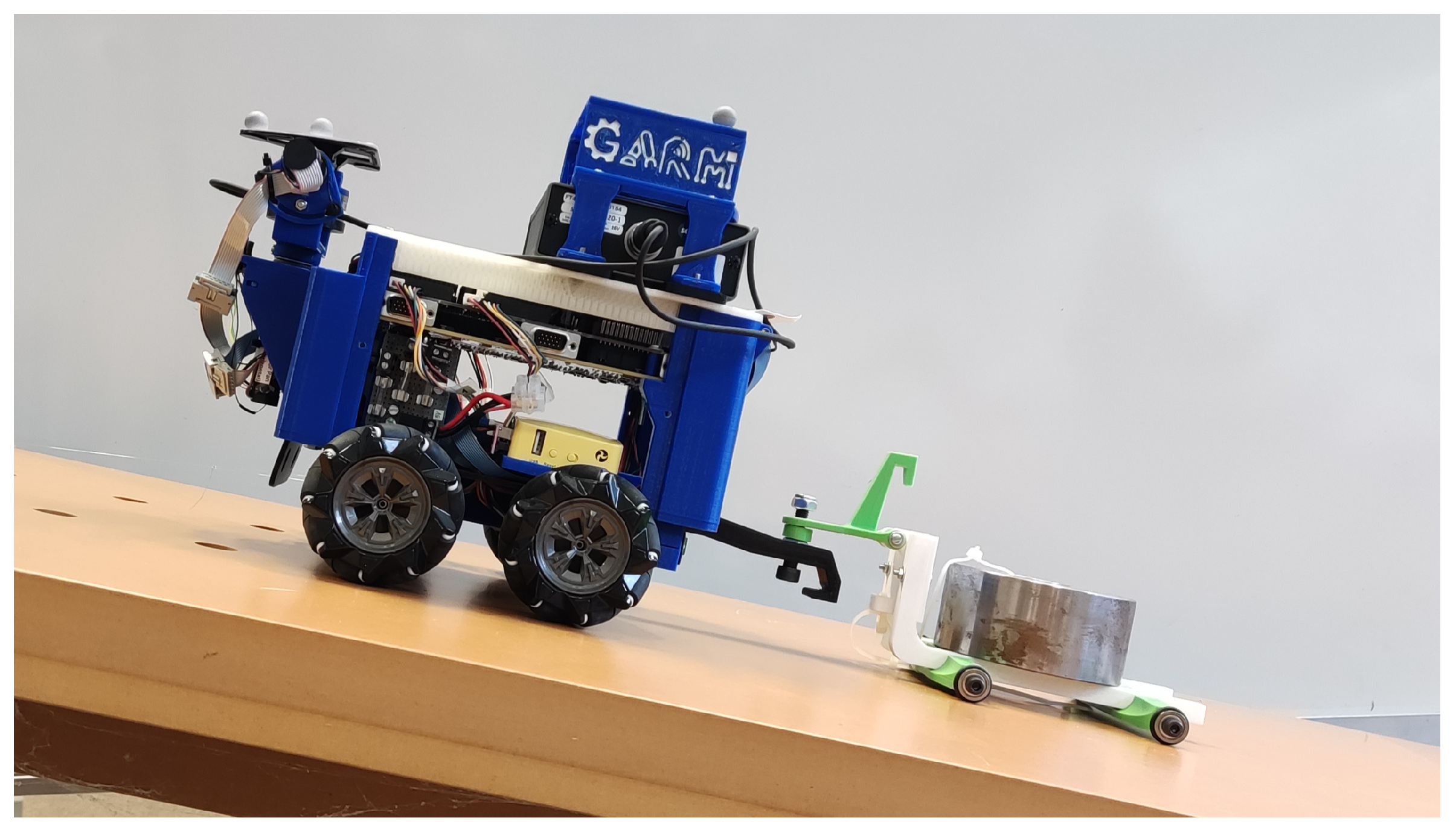
To prove the goodness of the new control scheme, a disturbance d is generated. According to (8), the disturbance d depends on the terrain slope ($\alpha$), the robot mass (M) and the wheel’s radius (R). Thus, a large input disturbance is generated adding an extra payload to the robot and testing it on an $\alpha ={15}^{\circ }$ ramp. A trailer is designed to carry the extra payload. The connecting rod between the trailer and the robot is designed to apply the force of the payload just at the same height as the motor axle plane. This design prevents the application of an undesirable rolling torque to the robot that might change the robot dynamics. The original mass of the robot is $M=3.8$ kg and the total extra payload added is $3.28$ kg, which adds up to $\widehat{M}=7.08$ kg, which is around an $86\%$ increase. Figure 8 shows the robot over the ramp holding the payload over the designed trailer.

7.2. Compensators to Overcome Nonlinearities

As previously mentioned in Section 4.2, the system exhibits several nonlinearities, including the nonlinear motor friction, saturation and encoder resolution. Among them, nonlinear friction can be compensated by means of a friction compensator block ($FC$) of the form

$$V_c\left(t\right)=\left\{\begin{array}{cc}{V}_c(t-T_s),\hfill & \left|e\left(t\right)\right|\le e_{min}\hfill \\ V_f^{min}·sign\left(V_r\left(t\right)\right),\hfill & \left|e\left(t\right)\right|>e_{min}and\left|V_r\left(t\right)\right|+V_f^K\le V_f^{min}\hfill \\ V_r\left(t\right)+V_f^K·sign\left(V_r\left(t\right)\right),\hfill & \left|e\left(t\right)\right|>e_{min}and\left|V_r\left(t\right)\right|+V_f^K>V_f^{min}\hfill \end{array}\right.$$

(38)

where $V_c\left(t\right)$ is the output voltage of the compensator; $V_r\left(t\right)$ is the control signal; $e\left(t\right)$ is the error signal measured between the input reference ${\theta }^{*}\left(t\right)$ and the output encoder measure $\theta \left(t\right)$; $e_{min}$ is a defined error band; $V_f^{min}$ is the minimum voltage supplied to the motor, which has been set to 0.9 V, just slightly greater than the stiction break-away voltage $V_f^S$, to ensure a value outside the motor dead-zone; and $T_s$ is the sample time of the system (25 ms). The error band $\pm e_{min}$ is established to avoid motor oscillations when reaching the reference due to the motor dead-zone and its compensation, determined by the minimum angular displacement that the motor can turn. This value is determined by applying the minimum voltage to move the motor, $V_f^{min}$, in $t=T_s=25$ ms, obtaining a conservative value of ±2 encoder pulses, which corresponds to $e_{min}$ = ±2.4° in each wheel. Note that, in this threshold, the quantisation error introduced by the encoder is also included.

This $FC$ is the same as the one designed in [12], except for the first equation of the piecewise function. Originally, the output value of the compensator was set to zero when $\left|e\left(t\right)\right|\le e_{min}$. Now, the output value is the voltage that was delivered in the previous instant, $V_c\left(t\right)=V_c(t-T_s)$, to keep the motor pushing in the case that a disturbance affects the system.

7.3. Results and Comparison with the Previous Control Scheme

The previous control scheme developed in [12] is composed of a $PID$ controller plus a prefilter combined with a Smith predictor, an antiwindup scheme and a friction compensator. The prefilter is designed to cancel the zeros introduced by the regulator in the closed-loop system and also two poles, reducing the order of the closed-loop system to a second order. Thus, the combination of the $PID$ and the prefilter results in a second-order critically damped system where a double pole of the closed-loop system is placed in $p=-B_0/2\approx -10$. As the regulator is designed with an integral part ($PID$), an antiwindup scheme is needed to overcome motor saturation. Finally, the Smith predictor and the friction compensator cope with the time delay and nonlinear friction, respectively.

On the other hand, the new control scheme is composed of a $PD$ controller combined with a disturbance compensator, along with a Smith predictor and a friction compensator. As it was explained in Section 5.4, we have designed the regulator by placing a double pole in $p=-B_0/2\approx -10$ so as to finally obtain a critically damped second-order system. This regulator does not introduce any zeros in the closed-loop system, so no prefilter is needed. In this way, the new controller is equivalent to the previous one but is much simpler. The regulator has no integral part, so no antiwindup scheme is needed either. The Smith predictor is integrated into the system in addition to the compensator to reject the disturbances designed in Section 5.5, which was a missing feature in the previous control scheme. Finally, the new control scheme includes a friction compensator, which is essentially the same as the one designed in [12] but with a slight modification, as explained in the previous section.

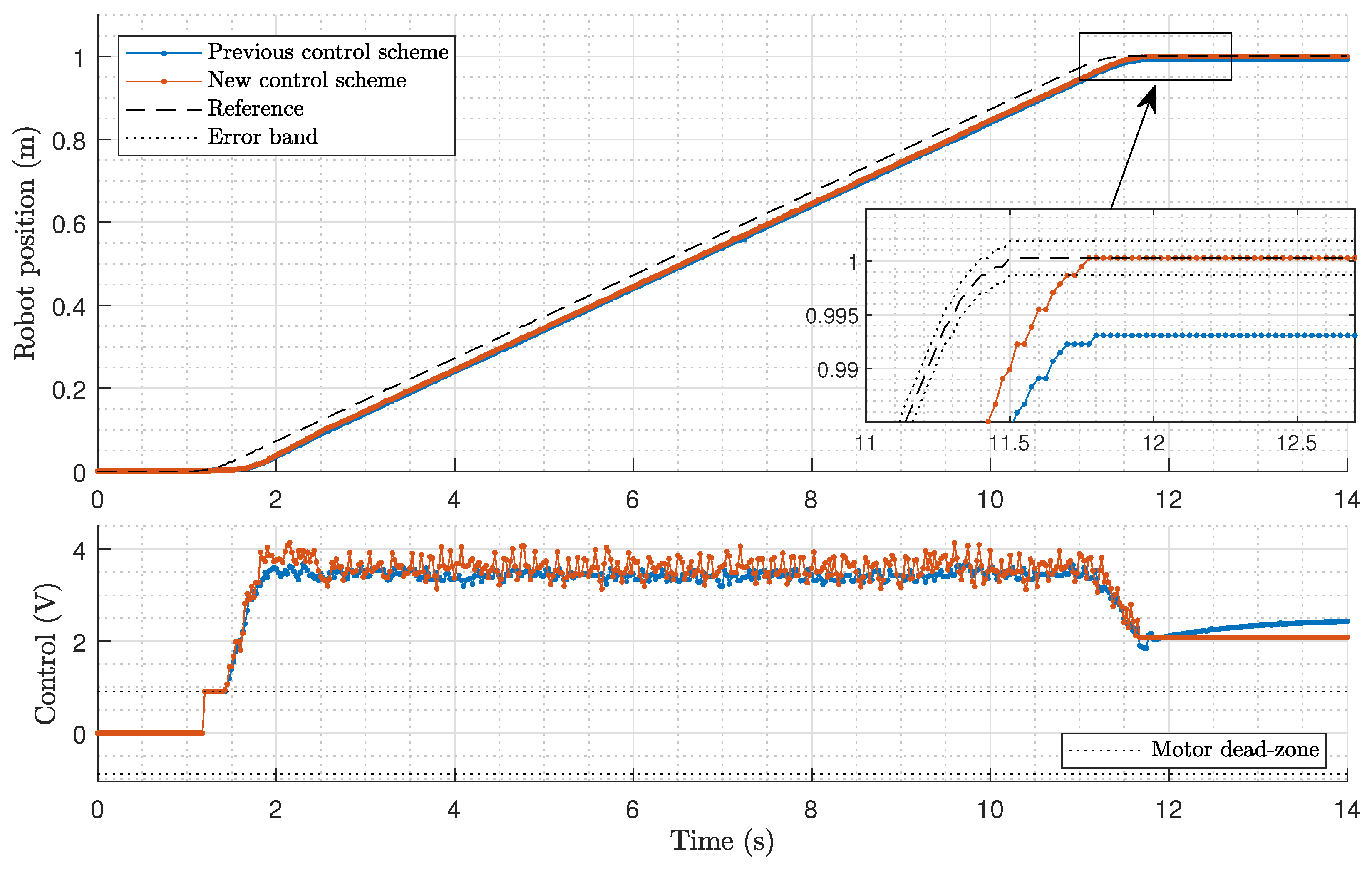
Figure 9 shows the results obtained from the experimentation, both the robot position (in meters) and control signal (in volts). Two experiments are represented. On the one hand, the blue line labelled as Previous control scheme shows the performance of the proposed controller in [12]. On the other hand, the red line labelled as New control scheme shows the response of the new control scheme proposed in this work.

The previous controller follows the designed trajectory but is not able to reach the desired ending position, as can be seen in the detailed view of the robot position. This is a consequence of the disturbance introduced by the slope and the payload, which affects the implemented Smith predictor. On the contrary, the new controller is able to reject the disturbance and the robot moves to the desired position, following the desired trajectory even better than the previous controller.

In order to measure quantitatively the improvement in the new controller compared with the previous one, two performance index are calculated. First, the steady-state error ($SSE$) at the end of the trajectory is measured. The experiments show that the $SSE$ of the previous controller is 7.18 mm, whereas the new controller performs nicely and gives an $SSE$ of 0 mm. The error band defined limits the $SSE$ to ±2 encoder pulses, which is equivalent to 1.6 mm in robot displacement. This means that the new controller performs perfectly, whereas the performance of the previous one is not acceptable, as it is not able to overcome the input disturbance. Finally, the root mean square error ($RMSE$) between the input reference and the robot position is calculated. This parameter gives a measure of how close to the reference signal the robot moves. Thus, the $RMSE$ of the previous control scheme is 27.54 mm, whereas the $RMSE$ of the new one is 23.09 mm. These results demonstrate that the new controller more closely follows the desired trajectory, as the $RMSE$ is 16.2% lower compared with the previous controller.

8. Conclusions

This paper has addressed the positioning of low-cost mobile robots under the effect of an unknown terrain slope. These robots have a hardware-induced delay and their actuators are integrating processes. Then, the standard Smith predictor could not remove the steady-state error caused by this slope. Moreover, the subsequent Smith predictor modifications designed to remove this steady-state error show inefficient transients. Thus, the contribution of this paper has been developing a new Smith predictor scheme that achieves a zero steady-state positioning error when the robot has to face an unknown slope while cancelling the transient error in a more efficient manner, i.e., a faster cancellation with a lower maximum error, than other Smith predictor control schemes.

A relevant conclusion of this paper is that $H\left(s\right)$ must have a zero at the origin of the complex plane in order to remove the steady-state error caused by a step disturbance. We mention that some recent works, e.g., [28,35], close an inner loop in the Smith predictor similar to ours by implementing a $PD$ controller in the $H\left(s\right)$ block. Choosing such $PD$ controllers for $H\left(s\right)$ is not the most efficient solution to remove the error caused by step disturbances because they do not have a zero at the origin and, then, they cannot achieve a zero steady-state error. It sometimes forces the addition of other control elements in order to cancel the permanent error.

Moreover, the controller embedded in our Smith predictor does not need to be integrating to compensate for a terrain slope disturbance. According to this, this paper has carried out a theoretical analysis, simulations and experiments that show that a simple P controller (1) does not introduce zeros that could produce overshoot in the response (as a $PID$ could do), (2) does not need the help of an antiwindup system to avoid overshoots caused by actuator saturation, as it would be the case if an integrating controller were used, and (3) the robustness to changes in the plant parameters is significantly lower than that of the standard $SP$ scheme.

Regarding the robustness issue of the $SP$-H, it is close to the robustness of the $SP$ with the $PID$ of [12] in an acceptable range of frequencies, and this robustness is enough to guarantee stability in the range of working conditions of our robot. However, this robustness could be improved by increasing the parameter $\lambda$ of $H\left(s\right)$.

Finally, we mention that, though we have used a P controller to prove the main features of our control scheme, other non-integrating controllers could be used, like $PD$ controllers, that would allow us to freely allocate the two poles of the closed-loop system while the use of an antiwindup system is still avoided. We highlight the simplicity of our control system compared to others, like nonlinear controllers (e.g., sliding control).