Abstract
This paper proposes a path planning and tracking control algorithm for multi-autonomous mobile robot (multi-AMR) systems that addresses the challenges posed by AMRs with a kinematic model. The proposed path planning algorithm is divided into two layers. The upper layer of the algorithm detects spatiotemporal conflicts between the paths of any two AMRs using a spatiotemporal conflict detection tree and the Separating Axis Theorem. The lower layer of the algorithm takes into account the kinematic model of the AMRs, ensuring that the generated paths satisfy the nonholonomic constraints. Furthermore, the lower layer introduces weighted adjustments to the heuristic evaluation, significantly improving the efficiency of the planning process. The proposed tracking control algorithm accounts for the kinematic model of AMRs and various constraints, achieving precise path tracking through model predictive control. The simulation results demonstrate that the proposed path planning and tracking control algorithm can efficiently generate conflict-free paths and achieve precise tracking control that satisfies the nonholonomic constraints of multi-AMR systems.
1. Introduction
Ongoing technological advancements have led to a notable shift towards automation within the manufacturing industry [1]. This transition has seen a growing deployment of Autonomous Mobile Robots (AMRs) in industrial production and warehousing logistics systems [2]. The significance of path planning for AMRs cannot be understated, as these paths directly influence the efficiency and safety of the robots’ movements. Consequently, a critical challenge arises: devising effective and feasible paths for each AMR operating within a multi-AMR system that comply with their kinematic models while ensuring conflict avoidance throughout the entire path [3].
In the field of single AMR path planning, researchers have proposed a variety of algorithms, such as the Dijkstra algorithm, Greedy Best-First Search algorithm and A* algorithm, among others [4,5,6,7,8,9]. Multi-AMR systems, which feature several AMRs collaborating within the same scenario, exhibit greater complexity and challenges compared to single AMR systems. Various path planning algorithms have been devised for these systems, encompassing priority-based cooperative algorithms, AI-based algorithms, and conflict-search algorithms. The WHCA* algorithm enhances HCA* by implementing a windowed search strategy, which plans paths near the current place to reduce computational load. It also dynamically adjusts AMRs’ priorities based on window conditions, improving adaptability to environmental changes and interactions among AMRs [10,11,12]. However, these algorithms require maintaining communication among all AMRs for conflict detection. The PBS algorithm stratifies multi-AMR path planning into priority groups, allowing sequential planning where lower-priority AMRs adjust their paths based on those of higher-priority AMRs to prevent collisions [13]. In the realm of AI-based algorithms, the PRIMAL algorithm employs a distributed architecture that merges deep reinforcement learning with imitation learning for multi-AMR path planning [14]. Additionally, PRIMAL2 has the lifelong planning capability [15]. The MADDPG algorithm and the MAPPO algorithm cooperatively trains behaviors of other AMRs in continuous spaces, enabling collaborative decision-making among multi-AMR [16,17]. However, these algorithms require substantial amounts of data and computational resources for training and generally have lower interpretability. In conflict-search-based algorithms, the Conflict-Based Search (CBS) algorithm is a multi-layered strategy for multi-AMR path planning where the lower layer independently plans a path for each AMR, and the upper layer assigns spatiotemporal constraints by detecting conflicts among the lower layer’s path [18,19,20].
The AMR path tracking control method based on kinematic models can accurately and effectively design control strategies that meet the motion constraints of AMRs, improving the performance metrics of the system in completing operational tasks. Currently, various algorithms such as Proportional-Integral-Derivative (PID) control, Fuzzy Logic Control (FLC), and Model Predictive Control (MPC) have been developed. PID is a classic control algorithm that achieves precise control of the system by adjusting three parameters: proportional, integral, and derivative, but their performance is limited when dealing with nonlinear systems and multi-constraint problems [21]. FLC, based on fuzzy set theory, controls the system through fuzzy rules. FLC does not require precise mathematical models, and has good robustness and adaptability, but designing and adjusting fuzzy rules is relatively complex, and achieving precise control can be challenging [22]. MPC, as an advanced control strategy, has gained widespread attention for its significant advantages in handling multi-constraint optimization problems [23]. MPC can optimize the current control input by predicting the system’s behavior over a future time horizon in each control cycle, thus achieving precise control of complex systems. It can handle nonlinear systems and effectively cope with uncertainties and disturbances both inside and outside the system. Additionally, MPC excels in considering system dynamics and input–output constraints, ensuring safety and stability while maximizing system performance.
Addressing the path planning issues in multi-AMR systems, we enhance the CBS algorithm by proposing a multi-AMR path planning algorithm based on spatiotemporal conflicts and nonholonomic constraints. The algorithm employs a conflict detection tree integrated with the Separating Axis Theorem for precise collision detection, and efficiently plans feasible paths based on kinematic modeling for AMRs in a continuous space. Furthermore, we achieve precise tracking control of the planned paths based on the kinematic model of AMRs through the model predictive control algorithm. Our main contributions are summarized as follows:
- This paper develops a conflict detection tree integrated with the Separating Axis Theorem. It enables precise spatiotemporal conflict detection for each AMR’s path. This reduces the need for replanning and improves the efficiency of the algorithm.
- This paper introduces a path planning algorithm that incorporates kinematic models to plan feasible paths for each AMR. In the path planning process, factors required for actual AMR control are considered, addressing the issue of conflicts between AMRs caused by significant discrepancies between planning and control in multi-AMR systems. Moreover, building on this foundation, the algorithm’s heuristic function is weighted to further enhance planning efficiency by biasing the paths towards the goal.
- This paper takes the planning results of multi-AMR systems as the desired paths and, through the model predictive control algorithm, considers the specific kinematic models of the AMRs to achieve precise path tracking control.
2. Preliminaries and Problem Setting
In reality, AMRs need to consider their orientation and kinematic models to complete movements. The differences in orientation and kinematic models of AMRs also result in varying amounts of time and space required during path planning and tracking control. For example, Ackermann steering AMRs cannot turn in place and require additional space to turn. Therefore, the problem we need to solve is to achieve path planning and tracking control for multi-AMRs based on kinematic models.
2.1. Kinematic Model
This paper, we consider the orientation and kinematic model of Ackermann steering AMR to plan path. And, we achieve precise path tracking control based on this model.
The kinematic model of the Ackermann steering AMR as shown in Figure 1. The center of the AMR’s rear axle in the global coordinate system is . The yaw angle is . The AMR’s steering center is , and the front wheel steering angle is . The linear velocity v is controlled by the AMR’s rear wheels. In discrete time, the kinematic model of the Ackermann steering AMR in the global coordinate system is:
where L is the distance from the AMR’s front axle to its rear axle, and T is the time step. The coordinates of the AMR’s center position are:
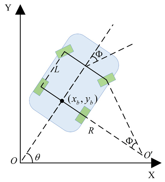
Figure 1.
The kinematic model of Ackermann steering AMR.
2.2. Problem Setting
In this paper, we define an enclosed warehouse space C, containing static obstacles O. We consider that there are some AMRs within this enclosed area. For , in the global coordinate system, the center position coordinates are , the yaw angle is , the start coordinate is , the goal coordinate is , and in discrete time, the path is . Let represent the position coordinates and yaw angle of at time t. denotes the space occupied by at that moment. represents the space occupied by static obstacles. As for the Ackermann steering AMR, define the front wheel steering angle as , the linear velocity as , the change in front wheel steering angle as , and the change in linear velocity as .
If a planned path P and a tracking control meet the following conditions, it is considered a feasible path:
- The planned path satisfies the nonholonomic constraints of the AMR;
- The AMR does not collide with any static obstacles while operating along the planned path, i.e., ;
- Any two AMRs operating on their respective planned path will not collide with each other, i.e., .
- The control inputs and their rate of change in the path tracking control algorithm meet the constraint conditions.
Considering the reasonableness of the problem, the following assumptions are made:
- The start and goal coordinates of different AMRs vary, and neither the start nor the goal positions collide with any static obstacles, i.e., ;
- The start and goal positions of any two AMRs do not collide, i.e., ;
- The initial position and orientation of the path tracking control algorithm are the same as the desired position and orientation, but the initial speed is zero.
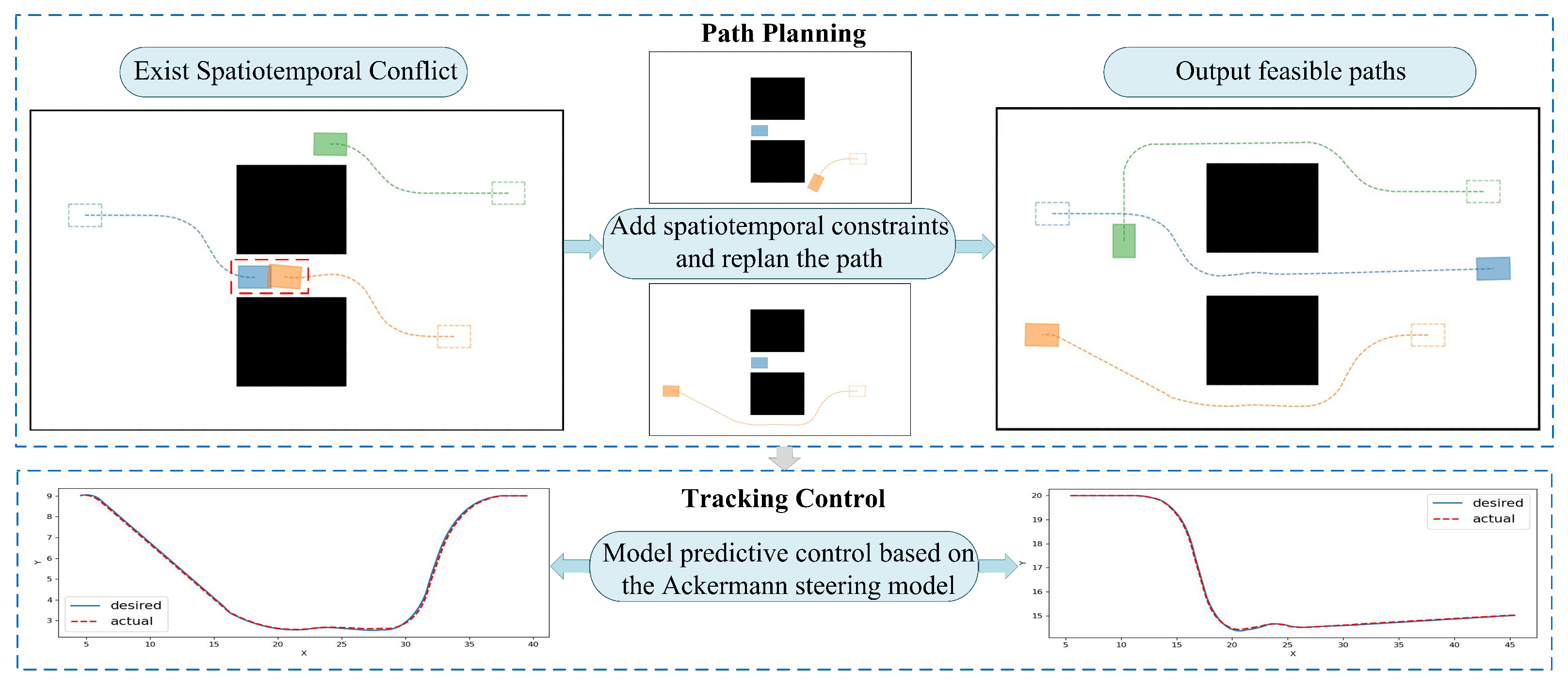
As shown in Figure 2, we improved the CBS algorithm by considering the kinematic model of AMRs, enabling path planning for a multi-AMR system. Additionally, we designed a model predictive control algorithm based on the kinematic model of AMRs to achieve precise tracking control. The goal is to plan conflict-free, feasible paths for all AMRs by considering their nonholonomic constraints and achieve precise tracking control.
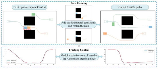
Figure 2.
A path planning and tracking control algorithm for Multi-AMR Systems based on spatiotemporal conflicts and nonholonomic constraints. The dashed rectangle represents the initial position of the AMR, while the filled rectangle represents the position of the AMR at a certain moment in time.
3. Path Planning Algorithm for Multi-AMR Systems
We enhanced the traditional CBS algorithm for the path planning of multi-AMR systems. At the lower layer, we employ an algorithm that considers spatiotemporal and nonholonomic constraints to plan feasible a path for an individual AMR. At the upper layer, a conflict detection tree integrated with the Separating Axis Theorem is used to precisely detect spatiotemporal conflicts in the planned paths of AMRs. The upper layer detects spatiotemporal conflicts and uses them as constraints for the lower layer algorithm, which is then called again to replan. This process is repeated until there are no conflicts between the paths. At this point, the algorithm successfully plans conflict-free, feasible paths that satisfy the nonholonomic constraints for all AMRs.
3.1. Spatiotemporal Conflict Detection Algorithm
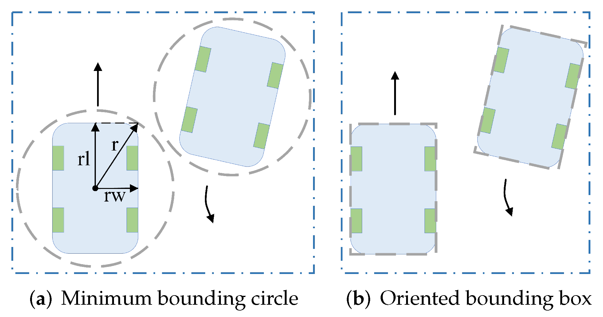
Generally, AMR conflict detection uses a minimum bounding circle. However, as shown in Figure 3, using a minimum bounding circle introduces excessive redundant space around the AMR. This excess can mistakenly identify nonconflicting AMRs as conflicting. Consequently, this increases the frequency of replanning and reduces the algorithm’s efficiency. Oriented Bounding Box (OBB) is a rectangular bounding box that adjusts according to the rectangle’s orientation. Since the actual shape of an AMR closely resembles a rectangle, this paper chooses the OBB to approximate the space occupied by an AMR.
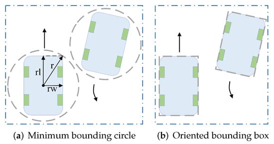
Figure 3.
Conflict situations of AMRs under two types of bounding boxes.
This paper employs the Separating Axis Theorem (SAT) for conflict detection with OBB [24]. By checking if the projections of two OBBs on any set of axes perpendicular to their edges overlap, it can be determined whether they are in conflict. Each OBB has vertices defined as , , , . The formula for calculating the actual coordinates of each vertex is
where represents the center coordinates of the OBB, which is the position of the AMR, and is the rotation angle of the OBB, corresponding to the yaw angle of the AMR. X and Y represent the coordinates of the vertices of the OBB in the local coordinate system. This equation converts the coordinates in the local coordinate system to the global coordinate system.
Then, calculate the normal vector from the vector formed by adjacent vertices and , where belongs to the set . The formula is
For and , their OBBs are denoted as and , respectively. Therefore, we define the sets and to contain all the normal vectors of and , respectively. The vector is any vector from the sets and . The result of the projection is
where represents the magnitude of the vector formed by vertex D and the origin in the x-direction, and represents the magnitude of the vector formed by vertex D and the origin in the y-direction. represents the magnitude of the normal vector in the x direction, and represents the magnitude of the normal vector in the y direction. Select any one of the normal vector from the two OBBs that require conflict detection. Project the vectors formed by all vertices D of and the origin, and the vectors formed by all vertices D of and the origin onto this normal vector , and take the minimum and maximum values of the projection positions to obtain the projection intervals and . If there exists such a normal vector , where , it indicates that the two OBBs are not in conflict. Otherwise, it indicates that the two OBBs are in conflict.
3.2. Path Planning Algorithm Based on AMR Kinematic Model
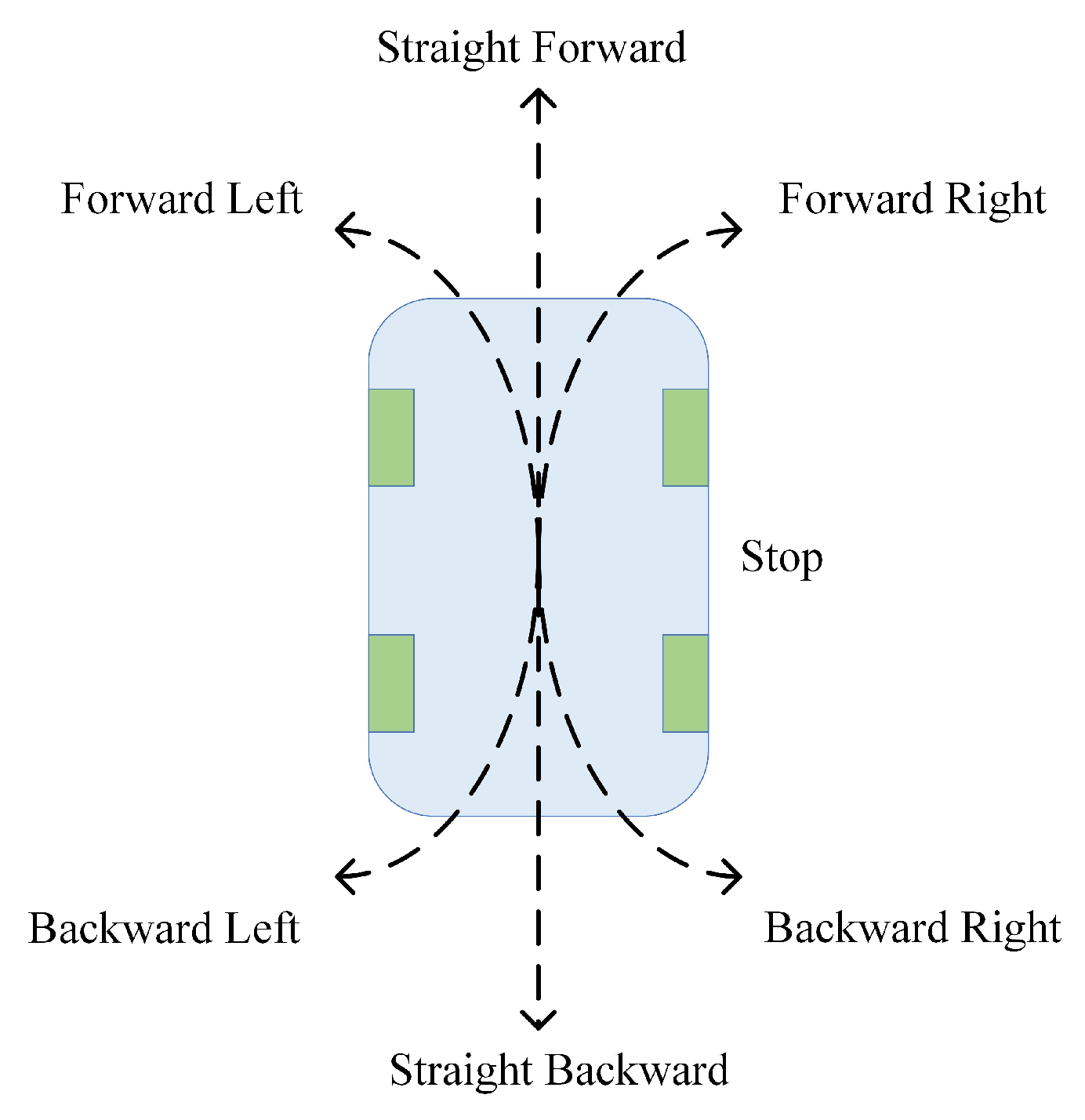
In this paper, we consider all the AMRs are the Ackermann steering AMRs. According to the kinematic model described in Figure 1, the motion modes of the Ackermann steering AMR studied in this paper are primarily categorized into seven types, as shown in Figure 4.
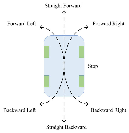
Figure 4.
The motion modes of the Ackermann steering AMR.
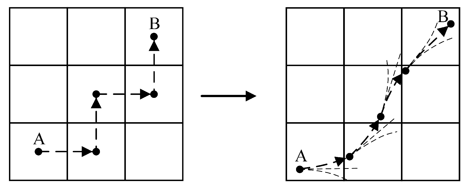
The Hybrid A* algorithm can plan paths based on the positions and orientations of points A and B, and ensures that the planned path adheres to the nonholonomic constraints of the AMR, as shown in Figure 5. Therefore, this paper modifies the Hybrid A* algorithm to plan feasible paths for Ackermann steering AMRs.
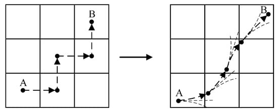
Figure 5.
The comparison of path planning between Hybrid A* algorithm based on kinematic models and traditional A* algorithm. A is the starting point of the path planning, and B is the endpoint of the path planning.
In this paper, we address the multi-AMR path planning problem by considering existing spatiotemporal constraints , extracted from the upper layer conflict detection tree, during AMR path planning. Consequently, by considering both spatial and temporal dimensions, the Hybrid A* algorithm is modified into a Spatiotemporal Hybrid A* algorithm. The nodes store information which includes , where p represents the position and yaw angle of the AMR in global coordinates, is the cost, and t is the time. In the Spatiotemporal Hybrid A* algorithm, the AMR extends from a node at time to a node at time t based on nonholonomic constraints, and performs interpolation between these two nodes for conflict detection. This node expansion is feasible, provided that the AMR’s path between the two nodes avoids conflicts with any static obstacles and sidesteps any existing spatiotemporal constraints extracted from the upper layer conflict detection tree. The constraint consists of multiple nodes, each in the form of , where represents the start time of the constraint, which lasts for 0.1 s. , , and represent the central position and orientation angle of the constraint, while and represent the length and width of the constraint, respectively.
Additionally, by incorporating a temporal dimension, the Spatiotemporal Hybrid A* algorithm produces more expanded nodes and has a slower planning speed. Therefore, we increase the weight of heuristic estimated costs, the algorithm is more oriented towards searching in the direction of the goal point, thus reducing the search space and accelerating the search speed. Based on this, the Spatiotemporal Hybrid A* algorithm is modified into a Weighted Spatiotemporal Hybrid A* algorithm. In this paper, the pseudocode for the path planning algorithm based on AMR kinematic model we propose is shown in Algorithm 1.
| Algorithm 1 Path planning algorithm based on AMR kinematic model |
|
The calculation formula for the cost function at node n is:
where is the heuristic cost at the node, is a constant weighting factor for the heuristic cost, and is the actual cost at the current node.
To align the planned paths with practical scenario requirements, we change the components of the cost function. The node information is , where is the front wheel steering angle of the AMR. The calculation formula for is
where represents the cost of each time step T. represents the cost of the front wheel steering angle , where a larger steering angle results in a higher cost. represents the cost resulting from changes in the front wheel steering angle, where a greater difference between the steering angle of the current step and the previous step leads to a higher cost. represents the actual cost of the current node. To ensure that the AMR moves in a straight line as much as possible, reducing the number of turns, changes in direction, and reversals, weights are applied to , , and , increasing the costs associated with turning, changing direction, and reversing. is the weight for reversing, is the weight for turning, and is the weight for changing direction. The values of , , and are all greater than 1. represents the cumulative cost generated by the historical actions prior to the current step.
4. Path Tracking Control Algorithm for Multi-AMR Based on Model Predictive Control
In this section, the path planned by the algorithm in the previous section is used as the desired path. By considering the kinematic model of Ackermann steering AMR, the tracking control is implemented based on the MPC algorithm. This ensures that, in a multi-AMR scenario, each AMR can accurately follow the path to complete its task.
For Ackermann steering AMR, for its kinematic models, the nonlinear equation is linearized using a first-order Taylor expansion at point , , , , and . The linearized formula is
After discretization using the forward Euler method, the formula is
At this point, the simplified form of the above formula is
where state vector , state matrix , input matrix , input vector .
We have simplified the linearized discrete formulas of the Ackermann steering AMR. Then, we will design the predictive formulas.
We define the change in the input vector as , and combining the state vector and control vector results in . And, we merge the state matrix and input matrix to construct a new state matrix and a new input matrix , where is the zero matrix, is the identity matrix, m is the length of the control vector, and n is the length of the state vector. Then, we obtain the predictive formula and decompose the state vector and control vector,
where .
Finally, we construct the cost function and the constraints. For Ackermann steering AMR, the formula is
In the cost function of the algorithm, represents the state error, denotes the change in control input, Q is the weighting matrix for the state error, and R is the weighting matrix for the change in control input. N represents the prediction horizon, and , , , and represent the front wheel steering angle, velocity, front wheel steering angle change, and acceleration, respectively. Each of these variables is subject to upper and lower bound constraints. By minimizing the cost function within the existing constraints and over a finite prediction horizon, a balance between the state error and control input is achieved.
By solving the cost function, the optimized control input is obtained, which then controls the AMR’s movement. This optimization process is repeated based on the latest state, forming a closed-loop control to achieve the desired path tracking.
5. Simulation
In this paper, we use Python for simulation experiments. To verify the effectiveness of the algorithm, we conducts tests in two different scenarios: a without obstacle scenario and a random obstacle scenario, with the number of AMRs in each scenario being 5, 10, and 15, respectively. And the sizes of the scenario maps are 50 × 50, 80 × 80, and 100 × 100 m, respectively. In the random obstacle scenario, the number of obstacles are 10, 20, and 40, respectively.
We use the Priority-Based Search algorithm (PBS), the Spatiotemporal Hybrid A* Conflict-Based Search algorithm (STH-CBS), and the Weighted Spatiotemporal Hybrid A* Conflict-Based Search algorithm (WSTH-CBS) to solve the multi-AMR path planning problem. Further, we define the distance between the start and goal points of each AMR is not less than half of the map’s length. To test the improvement in planning efficiency of the algorithm proposed in this paper compared to the PBS algorithm, we conduct five tests for each type of scenario map. The average of these test results represents the actual performance of the algorithm, as shown in Table 1.

Table 1.
The comparison of planning times for different algorithms in Multi-AMR systems.
According to test results, the STH-CBS and WSTH-CBS algorithms, which are improvements based on CBS, have higher planning efficiency than the Priority-Based Search (PBS) algorithm. Additionally, as the number of AMRs planned increases and the scenarios become more complex, the PBS algorithm faces an overload of spatiotemporal constraints for later planned AMRs, leading to fewer feasible paths and thus lower planning efficiency compared to the other two algorithms.
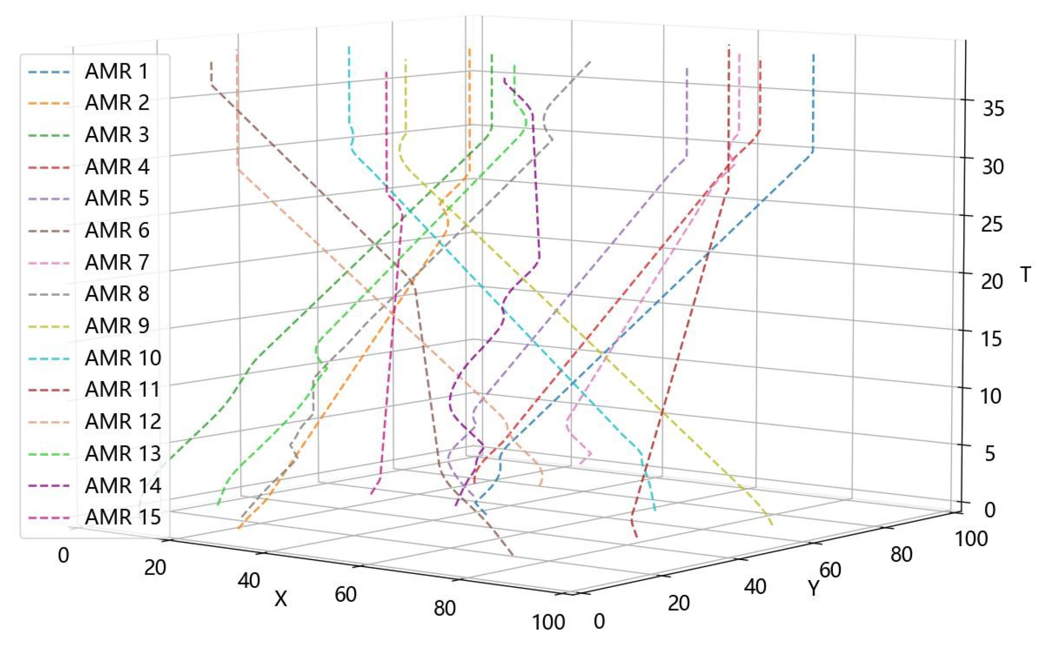
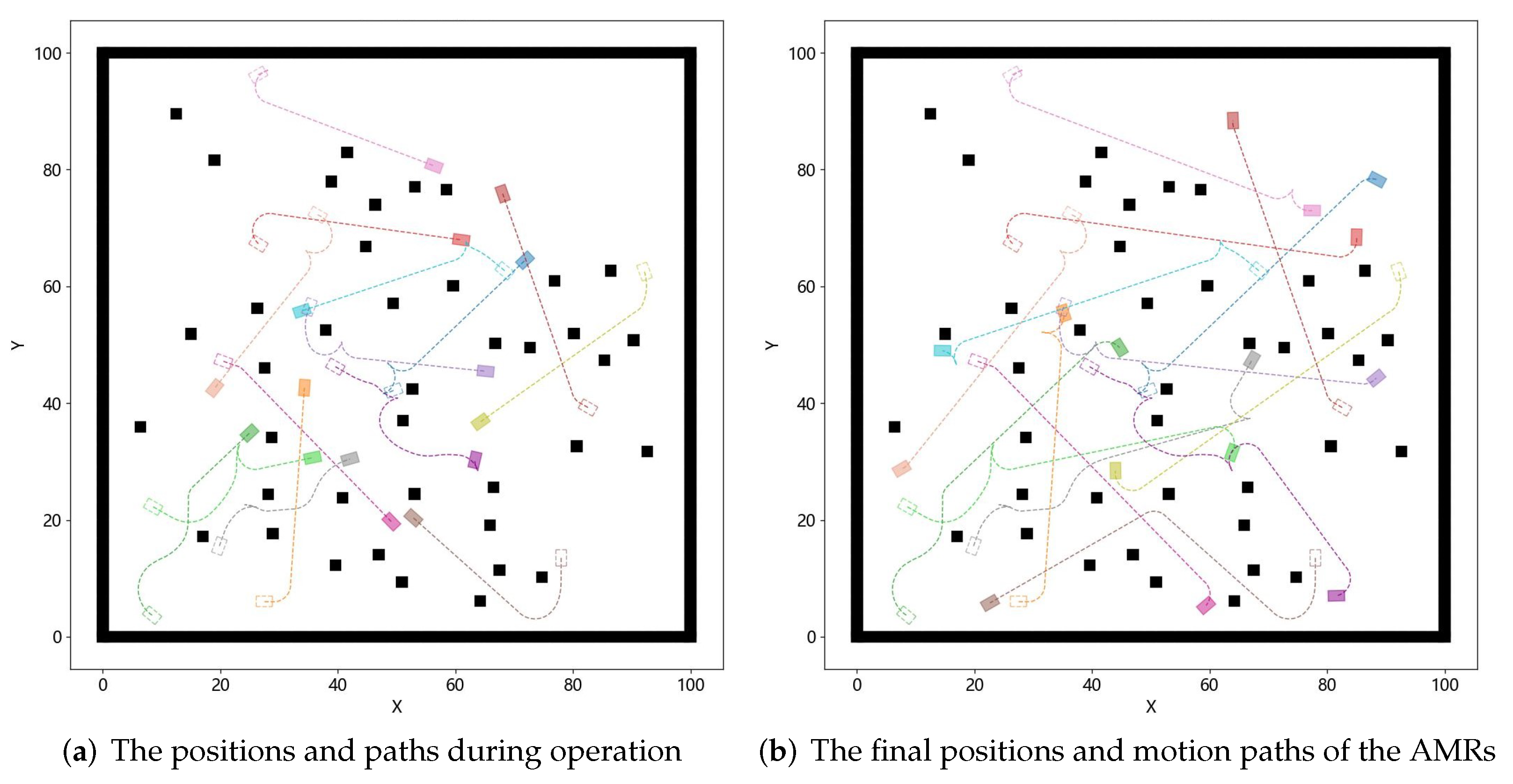
Figure 6 shows the paths of AMRs planned using the WSTH-CBS algorithm in a 100 × 100 random obstacle scenario. Figure 7 captures the positions at different moments from Figure 6, where Figure 7a shows the positions and paths during the AMRs’ operation, and Figure 7b shows the final positions and motion paths of the AMRs. The black areas represent the static obstacles, and the rectangles represent the Ackermann steering AMRs. Dashed rectangles and squares represent the starting positions of the AMRs, and filled rectangles and squares of the same color represent the current positions of the AMRs. The dashed line between the starting and current positions represent the motion paths of the AMRs.
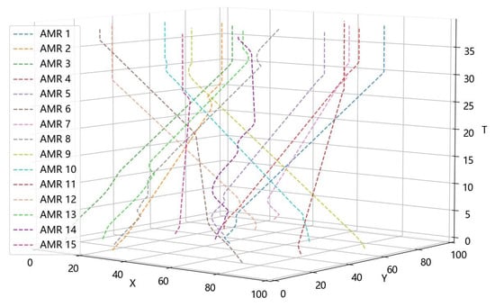
Figure 6.
Spatiotemporal paths of AMRs in a 100 × 100 random obstacle scenario.
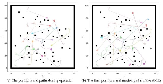
Figure 7.
Positions of AMRs at different times in a 100 × 100 random obstacle scenario. The dashed rectangle represents the initial position of the AMR, while the filled rectangle represents the position of the AMR at a certain moment in time.
Based on the paths of all AMRs obtained in Figure 7b, we perform tracking control using the MPC algorithm. In Figure 7b, AMR4 and AMR13 are selected as the example. Figure 8 shows the tracking results achieved through MPC control. Specifically, Figure 8a presents the tracking result for AMR4, and Figure 8b presents the result for AMR13. The MPC algorithm parameters are shown in Table 2. The blue curve represents the desired path obtained from the path planning algorithm, while the red curve represents the actual path achieved through MPC control. It can be observed that the red curve almost completely overlaps with the blue curve, demonstrating the effectiveness of the proposed planning and control algorithms.

Figure 8.
The path tracking control results based on the model predictive algorithm.

Table 2.
MPC algorithm parameter.
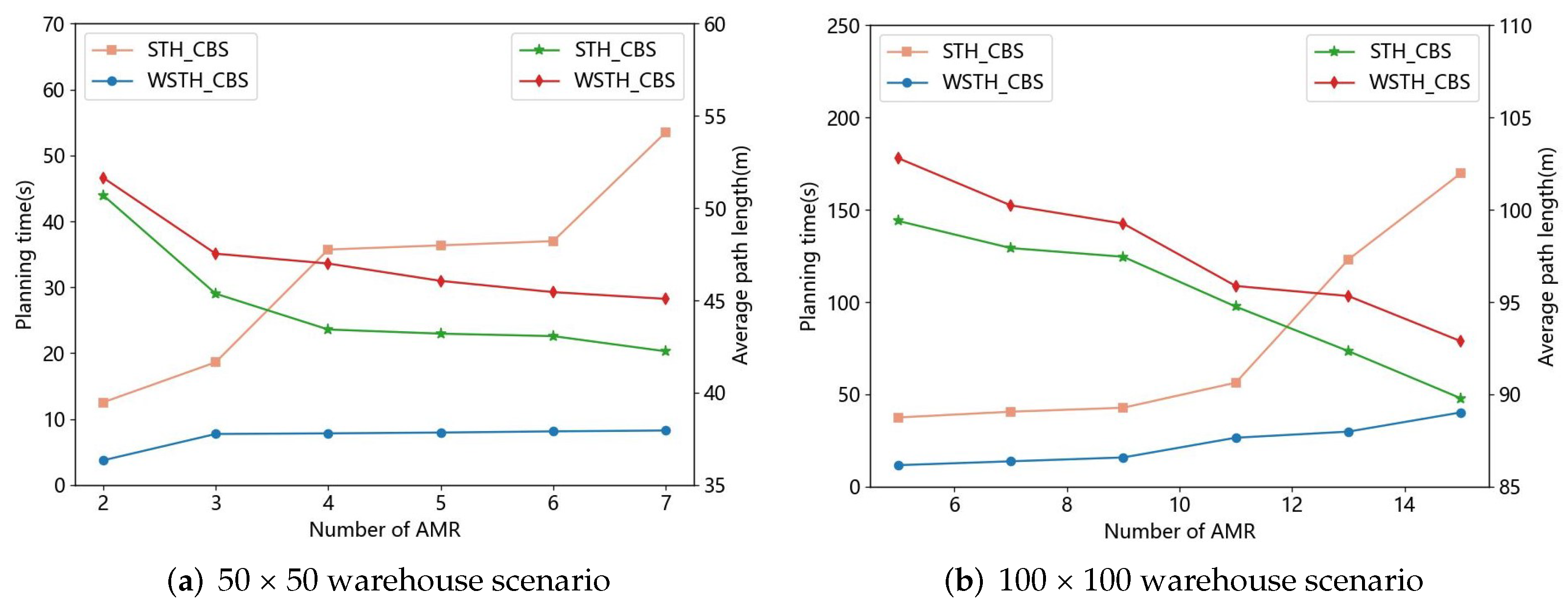
To evaluate the performance of the STH-CBS and WSTH-CBS algorithms, further simulation experiments are conducted in the warehouse scenario. The sizes of the warehouse scenario are 50 × 50 and 100 × 100. In this paper, we gradually increase the number of AMRs and compare the performance of the algorithms in terms of planning time and average path length. The planning time is the total time required for all AMRs to find feasible paths, where the less time reflects the higher algorithm efficiency. The average path length is the mean value of the path lengths traveled by each AMR, where a smaller average reflects a better overall planning solution. The comparison results of the algorithms are illustrated in Figure 9, where the horizontal axis represents the number of AMRs, the left vertical axis represents the planning time of the algorithms, and the right vertical axis represents the average path length planned by the algorithms. The orange and blue lines represent the planning times of the STH-CBS and WSTH-CBS algorithms, respectively. The green and red lines, respectively, represent the average path lengths planned by the STH-CBS and WSTH-CBS algorithms.
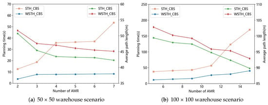
Figure 9.
The comparison of the planning times and the average path lengths for different algorithms in warehouse scenarios.
In the 50 × 50 warehouse scenario, the number of AMRs starts at two and increases by one each time, until it reaches seven, as shown in Figure 9a. In six simulation experiments, the average planning time for the STH-CBS algorithm is 32.29 s, and the average path length is 44.67 m; for the WSTH-CBS algorithm, the average planning time is 7.28 s, and the average path length is 47.13 m. Compared to the STH-CBS algorithm, the WSTH-CBS algorithm experiences a 5.51% increase in average path length, but the average planning time decreases by 77.45%.
In the 100 × 100 warehouse scenario, the number of AMRs starts at five and increases by two each time, until it reaches fifteen, as shown in Figure 9b. In six simulation experiments, the average planning time for the STH-CBS algorithm is 78.34 s, and the average path length is 95.28 m; for the WSTH-CBS algorithm, the average planning time is 22.95 s, and the average path length is 97.73 m. Compared to the STH-CBS algorithm, the WSTH-CBS algorithm experiences a 2.57% increase in average path length, but the average planning time decreases by 70.7%.
Based on the results of simulation experiments conducted on different sizes of warehouse scenario maps, the average path length planned by the WSTH-CBS algorithm is slightly longer than that of the STH-CBS algorithm. However, the WSTH-CBS algorithm shows a significant improvement in path planning efficiency.
To test the performance of the proposed algorithm in a warehouse environment, additional simulations were conducted on a 50 × 50 m scenario map with seven AMRs. An additional path planning algorithm, combining Bezier curves and the CBS algorithm (B-CBS), was introduced as a comparison method. This algorithm first uses the CBS algorithm to plan paths for each AMR on a discrete grid map, then smooths the paths using Bezier curves, and finally controls the AMRs to move simultaneously along the smoothed paths. The path planning success rate of this algorithm was then compared with that of the proposed algorithm. The path planning success rate is defined as the probability that all AMRs successfully avoid each other from the start to the goal. A higher success rate indicates better algorithm performance.
As shown by the data in Table 3, the B-CBS algorithm requires curve smoothing to meet control requirements, which results in significant deviations between the planned path and the tracking control trajectory, thereby reducing the success rate. In contrast, the proposed algorithm, which is based on the kinematic model of the AMR, enables precise tracking control, achieving a consistent success rate of 100%, thus demonstrating the effectiveness of the proposed algorithm.

Table 3.
Comparison of success rates in a 50 × 50 warehouse environment.
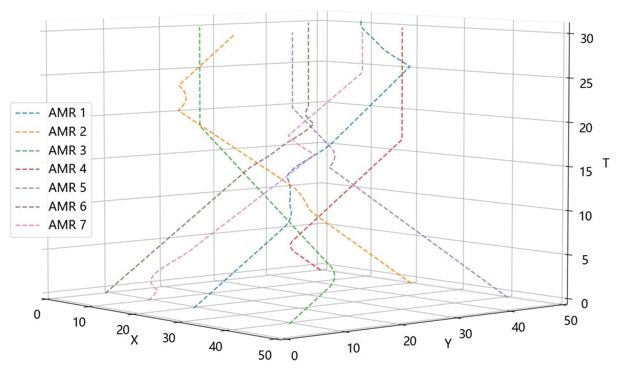
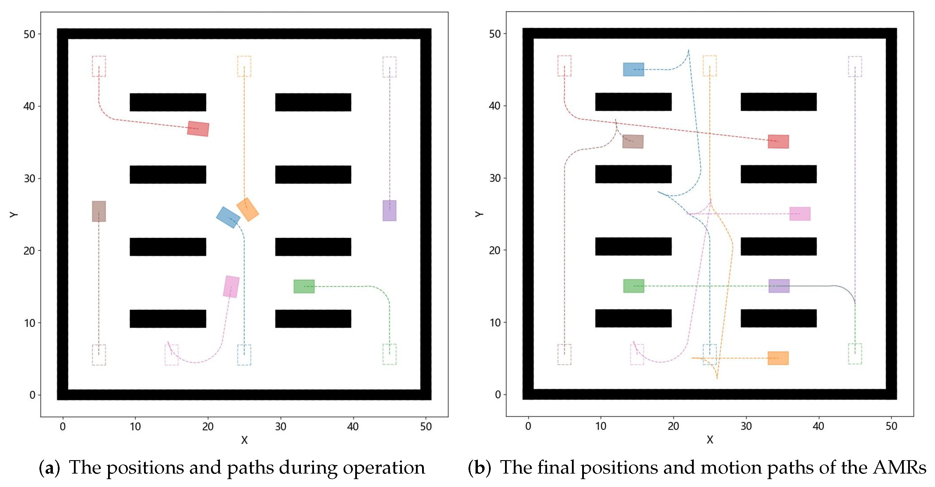
Figure 10 shows the paths of AMRs planned using the WSTH-CBS algorithm in a 50 × 50 warehouse scenario. Figure 11 captures the positions at different moments from Figure 10, where Figure 11a shows the positions and paths during the AMRs’ operation, and Figure 11b shows the final positions and motion paths of the AMRs. The rectangles represent the Ackermann steering AMRs. As shown in Figure 11a, the blue AMR changes its direction by turning to the left side to avoid a conflict with the orange AMR. At the same times, the orange AMR changes its direction by turning to the right side to avoid a conflict with the blue AMR.
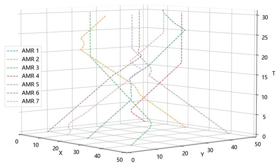
Figure 10.
Spatiotemporal paths of AMRs in a 50 × 50 warehouse scenario.
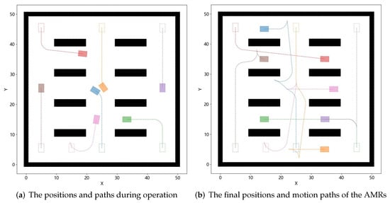
Figure 11.
Positions of AMRs at different times in a 50 × 50 warehouse scenario. The dashed rectangle represents the initial position of the AMR, while the filled rectangle represents the position of the AMR at a certain moment in time.
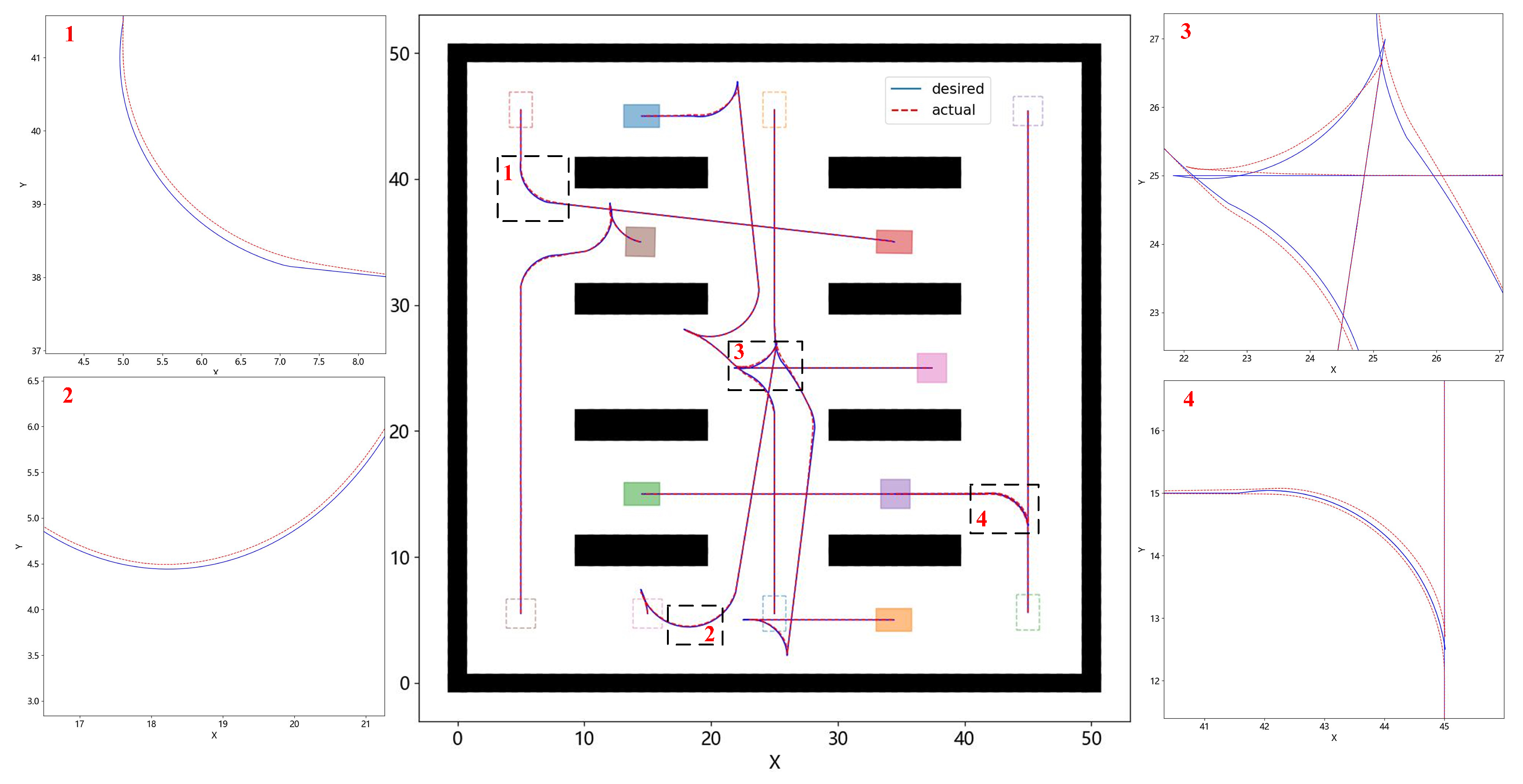
Based on the paths of all AMRs obtained in Figure 11b, we perform path tracking control using the MPC algorithm. For the Ackermann steering AMRs, we designed an MPC algorithm based on their models to perform path tracking control. Figure 12 shows the results of the path tracking. The blue curve represents the desired path obtained from the path planning algorithm, while the red curve represents the actual path achieved through the MPC algorithm. The black boxes highlight the paths of some AMRs during turning. By examining the magnified view of these sections, it can be observed that the red curve almost completely overlaps with the blue curve, with only minor control deviations during some turns.
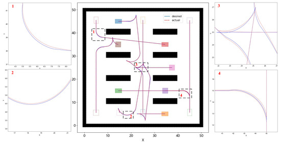
Figure 12.
Path tracking control results of AMRs in a 50 × 50 warehouse scenario.
The reason for the control deviations during turning is that, while controlling through the MPC algorithm, we considered the constraints on the upper and lower limits of the front wheel steering angle for the Ackermann steering AMR. Despite these constraints, the deviations between the actual path and the desired path are minimal. This demonstrates the effectiveness of the proposed planning and control algorithms in multi-AMR systems.
6. Conclusions
In this paper, we presented a novel path planning and tracking control algorithm for multi-AMR systems, specifically addressing the complexities introduced by kinematic models among AMRs. Our approach featured a two-layer path planning algorithm. The upper layer effectively identified spatiotemporal conflicts between the planned paths of any two AMRs using a spatiotemporal conflict detection tree combined with the Separating Axis Theorem. The lower layer of the algorithm takes into account the kinematic models of the AMRs, ensuring that the generated paths satisfy the nonholonomic constraints of each robot type. Furthermore, this layer enhanced heuristic evaluations with weighted adjustments, markedly improving planning efficiency. In addition, we developed a tracking control algorithm utilizing MPC. This algorithm precisely managed path tracking by considering the kinematic models and multiple constraints of the AMRs. Simulation results confirmed that our proposed approach successfully generated conflict-free paths while maintaining precise tracking control, fully adhering to the nonholonomic constraints of multi-AMR systems.
Looking ahead, the algorithm proposed in this paper can be further extended to differential drive and omnidirectional AMRs by adjusting the kinematic model. For differential drive AMRs, the primary difference in the kinematic model lies in its use of wheel speed differences to achieve turning. Therefore, the kinematic equations in the current path planning algorithm need to be modified by replacing the front wheel steering angle and linear velocity control of the Ackermann AMR with the speed control of the left and right wheels of the differential drive AMR, to accurately describe the motion characteristics of the differential drive. For omnidirectional AMRs, since they have the ability to move freely in any direction, their kinematic model is relatively simple, and does not require complex steering control. It is even possible to directly control the translational velocities in the x and y axes independently from the angular velocity, further optimizing the efficiency and flexibility of path generation. With these adjustments, the proposed algorithm can adapt to the kinematic models of different types of AMRs, expanding its range of applications and providing efficient path planning and control solutions for multi-robot systems in various real-world scenarios.
Author Contributions
Writing—original draft, Z.S.; Writing—review and editing, L.Y.; validation, H.D.; form analysis, W.Z.; project administration, M.Z. All authors have read and agreed to the published version of the manuscript.
Funding
This work was supported by the National Natural Science Foundation of China under Grants No. 62073113, No. 62003122, and the Natural Science Foundation of Anhui Province under Grants No. 2208085UD15.
Data Availability Statement
The original contributions presented in the study are included in the article, further inquiries can be directed to the corresponding author.
Acknowledgments
We would sincerely want to thank the peoples who are supported to do this work and reviewing committee for their estimable feedback.
Conflicts of Interest
The authors declare no conflicts of interest.
References
- Ren, Z.; Rathinam, S.; Choset, H. A Conflict-Based Search Framework for Multiobjective Multiagent Path Finding. IEEE Trans. Autom. Sci. Eng. 2023, 20, 1262–1274. [Google Scholar] [CrossRef]
- Hou, Y.; Ma, Z.; Pan, Z. Online Multi-Agent Task Assignment and Path Finding with Kinematic Constraint in the Federated Internet of Things. IEEE Trans. Consum. Electr. 2024, 70, 2586–2595. [Google Scholar] [CrossRef]
- Hua, Y.; Wang, Y.; Ji, Z. Adaptive Lifelong Multi-Agent Path Finding with Multiple Priorities. IEEE Robot. Autom. Lett. 2024, 9, 5607–5614. [Google Scholar] [CrossRef]
- Wang, J.; Li, Y.; Li, R.; Chen, H.; Chu, K. Trajectory planning for UAV navigation in dynamic environments with matrix alignment Dijkstra. Soft Comput. 2022, 26, 12599–12610. [Google Scholar] [CrossRef]
- Jesuthas, N.J.A.; Somaskandan, S. Path-finding and Planning in a 3D Environment an Analysis Using Bidirectional Versions of Dijkstra’s, Weighted A*, and Greedy Best First Search Algorithms. In Proceedings of the 2nd Asian Conference on Innovation in Technology (ASIANCON), Ravet, India, 26–28 August 2022; IEEE: New York, NY, USA, 2022; pp. 1–8. [Google Scholar]
- Liu, S.; Liu, S.; Xiao, H. Improved gray wolf optimization algorithm integrating A* algorithm for path planning of mobile charging robots. Robotica 2024, 42, 536–559. [Google Scholar] [CrossRef]
- Kim, S.; Likhachev, M. Path planning for a tethered robot using Multi-Heuristic A* with topology-based heuristics. In Proceedings of the International Conference on Intelligent Robots and Systems (IROS), Hamburg, Germany, 28 September–3 October 2015; IEEE: New York, NY, USA, 2015; pp. 4656–4663. [Google Scholar]
- Cohen, L.; Greco, M.; Ma, H.; Hernandez, C.; Felner, A.; Kumar, T.K.S.; Koenig, S. Anytime Focal Search with Applications. In Proceedings of the 27th International Joint Conference on Artificial Intelligence (IJCAI), Stockholm, Sweden, 13–19 July 2018; Morgan Kaufmann: Burlington, MA, USA, 2018; pp. 1434–1441. [Google Scholar]
- Dolgov, D.A.; Thrun, S.; Montemerlo, M.; Diebel, J. Path Planning for Autonomous Vehicles in Unknown Semi-structured Environments. Int. J. Robot. Res. 2010, 29, 485–501. [Google Scholar] [CrossRef]
- Liu, Y.; Chen, M.; Huang, H. Multi-agent Pathfinding Based on Improved Cooperative A* in Kiva System. In Proceedings of the 5th International Conference on Control, Automation and Robotics (ICCAR), Beijing, China, 19–22 April 2019; IEEE: New York, NY, USA, 2019; pp. 633–638. [Google Scholar]
- Bnaya, Z.; Felner, A. Conflict-Oriented Windowed Hierarchical Cooperative A*. In Proceedings of the International Conference on Robotics and Automation (ICRA), Hong Kong, China, 31 May–7 June 2014; IEEE: New York, NY, USA, 2014; pp. 3743–3748. [Google Scholar]
- Silver, D. Cooperative Pathfinding, AAAI. In Proceedings of the 1st Artificial Intelligence and Interactive Digital Entertainment (AIIDE), Marina del Rey, CA, USA, 1–3 June 2005; AAAI Press: Washington, DC, USA, 2005; pp. 117–122. [Google Scholar]
- Ma, H.; Harabor, D.; Stuckey, P.J.; Li, J.; Koenig, S. Searching with consistent prioritization for multi-agent path finding. In Proceedings of the 33th Artificial Intelligence and Interactive Digital Entertainment (AIIDE), Honolulu, HI, USA, 8–12 October 2019; AAAI: Washington, DC, USA, 2019; pp. 7643–7650. [Google Scholar]
- Sartoretti, G.; Kerr, J.; Shi, Y.; Wagner, G.; Kumar, T.K.S.; Koenig, S.; Choset, H. PRIMAL: Pathfinding via Reinforcement and Imitation Multi-Agent Learning. IEEE Robot. Autom. Lett. 2019, 4, 2378–2385. [Google Scholar] [CrossRef]
- Damani, M.; Luo, Z.; Wenzel, E.; Sartoretti, G. PRIMAL2: Pathfinding Via Reinforcement and Imitation Multi-Agent Learning—Lifelong. IEEE Robot. Autom. Lett. 2021, 6, 2666–2673. [Google Scholar] [CrossRef]
- Lowe, R.; Wu, Y.; Tamar, A.; Harb, J.; Abbeel, P.; Mordatch, I. Multi-agent actor-critic for mixed cooperative-competitive environments. In Proceedings of the 31st International Conference on Neural Information Processing Systems (NIPS), Long Beach, CA, USA, 4–9 December 2017; MIT Press: Cambridge, MA, USA, 2017; pp. 6382–6393. [Google Scholar]
- Zhan, G.; Zhang, X.; Li, Z.; Xu, L.; Zhou, D.; Yang, Z. Multiple-UAV Reinforcement Learning Algorithm Based on Improved PPO in Ray Framework. Drones 2022, 6, 166–179. [Google Scholar] [CrossRef]
- Sharon, G.; Stern, R.; Felner, A.; Sturtevant, N.R. Conflict-based search for optimal multi-agent pathfinding. Artif. Intell. 2015, 219, 40–66. [Google Scholar] [CrossRef]
- Yakovlev, K.S.; Andreychuk, A. Any-Angle Pathfinding for Multiple Agents Based on SIPP Algorithm. In Proceedings of the 27th International Conference on Automated Planning and Scheduling (ICAPS), Pittsburgh, PA, USA, 18–23 June 2017; AAAI: Washington, DC, USA, 2017; pp. 286–594. [Google Scholar]
- Barer, M.; Sharon, G.; Stern, R.; Felner, A. Suboptimal variants of the conflict-based search algorithm for the multi-agent pathfinding problem. In Proceedings of the 7th Annual Symposium on Combinatorial Search (SoCS), Prague, Czech Republic, 14–16 July 2014; AAAI: Washington, DC, USA, 2014; pp. 17–29. [Google Scholar]
- Karthik, R.; Menaka, R.; Kishore, P.; Aswin, R.; Vikram, C. Dual Mode PID Controller for Path Planning of Encoder Less Mobile Robots in Warehouse Environment. IEEE Access 2024, 12, 21634–21646. [Google Scholar] [CrossRef]
- Jayasiri, A.; Mann, G.K.I.; Gosine, R.G. Behavior Coordination of Mobile Robotics Using Supervisory Control of Fuzzy Discrete Event Systems. IEEE Trans. Syst. Man Cybern. Part B Cybern. 2011, 41, 1224–1238. [Google Scholar] [CrossRef] [PubMed]
- Worthmann, K.; Mehrez, M.W.; Zanon, M.; Mann, G.K.I.; Gosine, R.G.; Diehl, M. Model Predictive Control of Nonholonomic Mobile Robots Without Stabilizing Constraints and Costs. IEEE Trans. Control Syst. Technol. 2016, 24, 1394–1406. [Google Scholar] [CrossRef]
- Chen, S.; Wu, J.; Xiong, P.; Qi, W.; Liu, L.; Yang, W.; Wang, K.; Zhao, X.; Yang, X.; Bian, X. Thermal Conductivity Prediction of SiC/Silicone Rubber Composites Using Combined Separate Axis Theorem-Finite Element Model. IEEE Trans. Dielectr. Electr. Insul. 2024, 31, 31–39. [Google Scholar] [CrossRef]
Disclaimer/Publisher’s Note: The statements, opinions and data contained in all publications are solely those of the individual author(s) and contributor(s) and not of MDPI and/or the editor(s). MDPI and/or the editor(s) disclaim responsibility for any injury to people or property resulting from any ideas, methods, instructions or products referred to in the content. |
© 2024 by the authors. Licensee MDPI, Basel, Switzerland. This article is an open access article distributed under the terms and conditions of the Creative Commons Attribution (CC BY) license (https://creativecommons.org/licenses/by/4.0/).


