Design of an Optical Path Scanning Control System in a Portable Fourier Transform Spectrometer Based on Adaptive Feedforward–Nonlinear Proportional-Integral Cascade Composite Control

Abstract

In order to obtain highly accurate infrared spectra, the optical path scanning control system in a portable Fourier transform spectrometer (FTS) must be able to realize highly stable reciprocal scanning. To address the positional localization and speed fluctuation problems of optical path scanning control systems, an adaptive feedforward–nonlinear PI cascade composite control algorithm (AF-NLPI) is proposed. A physical model of an optical path scanning control system is established. Moreover, an adaptive feedforward compensator using a dynamic forgetting factor is proposed, and it was combined with a nonlinear PI cascade controller to form a composite controller. The control parameters were tuned using the atomic orbital search algorithm. Further, the simulation and experimental results demonstrate that the AF-NLPI can effectively improve the control accuracy and anti-interference ability of an optical path scanning control system in a portable FTS with high feasibility and practicality. By setting the scanning stroke of the system to 8 mm and scanning at 10 mm/s, the stability of the optical scanning speed reached 99.47% when controlled by the controller proposed in this paper, thus fulfilling the motion requirements for optical path scanning control systems.

1. Introduction

A portable Fourier transform spectrometer (FTS) is a high-resolution spectral detection instrument that can quickly detect gases, liquids, and powders through the spectral characteristics of substances in different wavebands [1,2,3]. FTSs have been widely used in the field of quantitative and qualitative analyses of substances, such as in hazardous gas analysis [4]. For example, there is a characteristic peak of ozone at 925–975 cm⁻¹ and a characteristic peak of water vapor at 800–900 cm⁻¹. Sulfur hexafluoride has multiple characteristic peaks at 900–1600 cm⁻¹, and sulfur hexafluoride leakage detection can be carried out through these characteristic peaks [5]. In order to adapt to practical needs, portable FTSs, such as handheld [6,7] and vehicle-mounted [8] FTSs, have emerged. The interferometer is the core component of an FTS, and the miniaturization of the interferometer is the key to its portability [9]. Due to portable FTS’s mobility needs, while the interferometer is miniaturized, the moving mirror in the interferometer is required to maintain a high control accuracy and a stable scanning speed [10,11], which is a key issue that must be addressed in the design of portable FTSs.

A VCM is a small-sized direct-drive motor with high acceleration, a fast response, and smooth force characteristics [12,13]. With a suitable feedback device, its positioning accuracy can easily reach the micron and nanometer levels [14]. In a portable FTS, small voice coil motors (VCMs) are mostly used to control the moving mirror to complete the scanning of the optical path [15]. At present, the control of VCMs is still dominated by PID control, but the robustness of classic PID controllers is poor, and it is difficult to reconcile the contradiction between rapidity and stability.

In order to improve the performance of optical path scanning control systems, many controllers have been proposed and applied to improve the stability of motion of the moving mirror. Shi et al. [16] designed a swing-type moving mirror mechanism with a flexible support, and they used the PID algorithm to control the movement of the moving mirror, making its scanning accuracy better than 98.4%. Ren et al. [17] studied an optical path scanning control system using CPLD to realize a fully digital incremental PID controller, which made the speed stability of the moving mirror better than 97% in the uniform scanning stage. Wang et al. [18] used DSP to implement the PID algorithm to control a linear motor, and the position accuracy of the moving mirror in the interferometer reached 0.1 μm. However, it is difficult for the classic PID to balance the stability and rapidity of a system, and it is difficult to achieve high-speed stability. A fuzzy PID controller was used to control a linear motor [19] and VCM [20]; an improved fuzzy controller was also proposed [21], and all achieved good results. However, there are many parameters of fuzzy PID controllers, and it is difficult to find an accurate fuzzy rule table. Guo et al. [22,23] used a permanent-magnet synchronous linear motor to drive a moving mirror and inserted a repetitive controller into the control system, which suppressed the periodic disturbance. However, repetitive controllers can only suppress periodic disturbances, and the system needs to run for several cycles to achieve good results. Li et al. [24] proposed an adaptive online genetic algorithm for tuning a PID controller, and the effectiveness of the control strategy was verified with a simulation. Shi et al. [25] adopted the double closed-loop PI algorithm to adjust an interference system modeled in the SABER environment, and the simulation verified the rationality of the modeling method and the effectiveness of the algorithm. Qu et al. [15] adopted an auto-disturbance rejection controller to control a VCM, which effectively reduced the influence of disturbance and enhanced the anti-disturbance capabilities of the system. However, the auto-disturbance rejection controller also faced the problem of parameter tuning [26]. Fractional-order PID controllers have good robustness and anti-interference abilities [27], and they have been widely used in optoelectronic systems [28] and servo systems [29]. However, fractional-order PID controllers have many parameters, and parameter tuning is difficult [30]. From the above references, it can be seen that, on the one hand, although the above-mentioned algorithms improved the performance of the systems, control systems are relatively complex and have many parameters, resulting in a large computational load. On the other hand, the position of the zero optical path difference and the position of the uniform-speed zone need to be considered in the data acquisition system of an FTS. The above algorithms mostly only controlled the speed of the VCM, and the application of multi-loop control was scarce.

Compared with the classic PID algorithm, the nonlinear PID algorithm can better adapt to nonlinear systems, and it has the advantages of a fast response, small overshoot, and small steady-state error [31,32]. Feedforward control can effectively suppress the impact of measurable but uncontrollable disturbances on a system in advance [33]. For systems with high-speed and high-precision motion requirements, the introduction of adaptive feedforward items into the system can effectively reduce the trajectory tracking error in the acceleration and deceleration stages [34]. Composite control is a control method that combines feedback control and feedforward control. It can combine the advantages of the two control algorithms and greatly improve the tracking accuracy of the servo system [35,36]. Therefore, this paper proposes an adaptive feedforward–nonlinear PI cascade composite (AF-NLPI) controller that can improve the control accuracy of a system while ensuring its rapid response, and the system’s adaptive capabilities are also enhanced. The AF-NLPI controller can balance the contradiction between the stability and rapidity of the system based on the error, and it can update the feedforward coefficient adaptively, quickly, and stably, improving the system’s steady-state anti-interference capabilities and its fast and dynamic convergence capabilities. The AF-NLPI controller is applied to an optical path scanning system, achieving stable scanning that meets the system requirements and effectively reduces the system’s following error.

The rest of this paper is organized as follows: Section 2 introduces the related problems of the optical path scanning system and derives the transfer function of the VCM. Section 3 focuses on the design of the AF-NLPI controller. This section is divided into three subsections to introduce the nonlinear PI cascade controller, the adaptive feedforward compensator, and tuning of controller parameters. Section 4 establishes a model of the optical path scanning system, outlines the conducted simulation experiments, and verifies the performance of the controller proposed in this paper by comparing it with a variety of controllers. Section 5 describes the experimental verification. The conclusions of this paper are provided in Section 6.

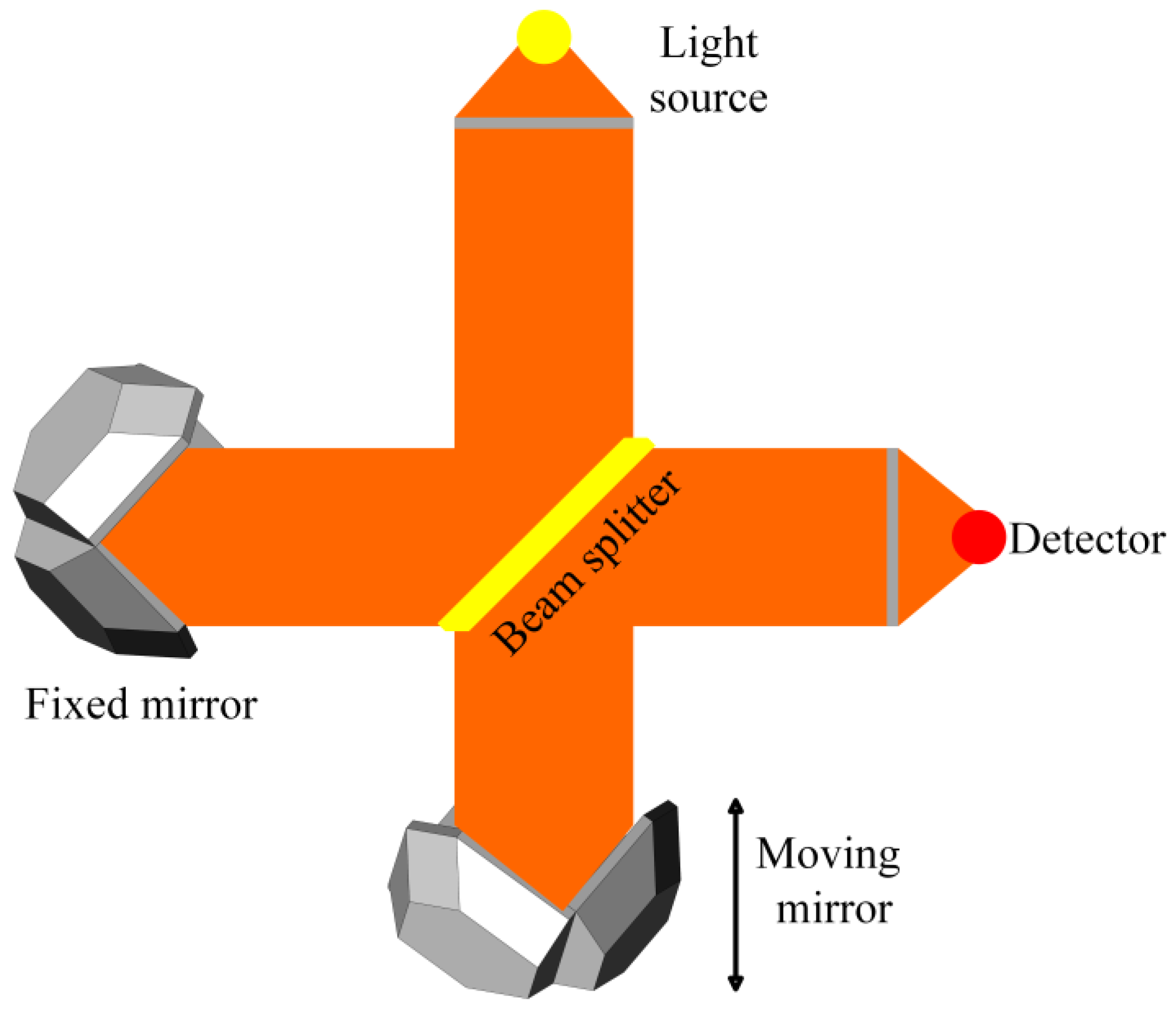
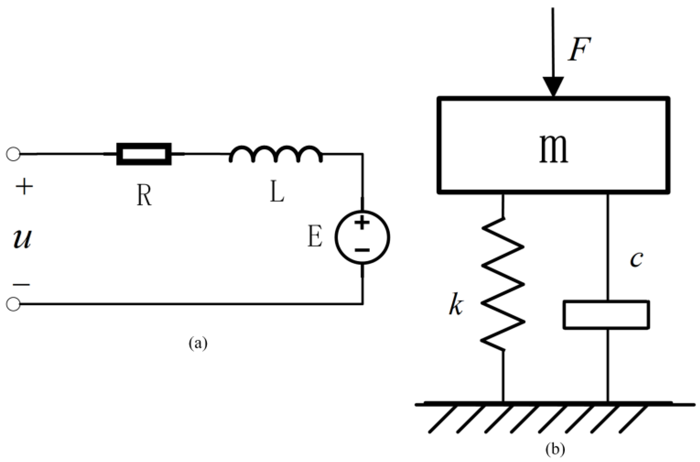
2. Problem Formulation of Optical Path Scanning System

The structure of the Michelson interferometer is shown in Figure 1. In a Michelson interferometer, the moving mirror moves at a constant speed to scan, thereby producing a frequency-stable interferogram. Assuming that the light source is monochromatic light with frequency $\sigma$, the moving mirror moving speed is $V$, and the frequency $f$ of the interferogram produced by the monochromatic light modulated is [37]:

$$f=2V\sigma .$$

(1)

If the motion speed of the moving mirror is unstable, the frequency of the interferogram will be changed, thereby affecting the quality of the spectrum retrieved from the interferogram. According to the reference, when the fluctuation of the optical path scanning speed is less than 2%, the influence of the fluctuation of the moving mirror speed on the quality of the spectrum is negligible [24].

The miniaturized VCM used in this study can be equivalent to a mass–spring–damper system. The electrical and mechanical models of the VCM under ideal conditions are shown in Figure 2, and its electrical balance equation and mechanical balance equation are [38,39]:

$$\left\{\begin{array}{l}u=E+iR+L{i}^{\prime }, E=BLv=k_e{x}^{\prime }\hfill \\ F=BLi=m{x}^{″}+c{x}^{\prime }+kx\hfill \end{array}\right.,$$

(2)

where $u$ is the armature voltage of the VCM, $E$ is the induced electromotive force of the VCM, $i$ is the armature current of the VCM, $k_e$ is the back EMF coefficient, $k$ is the elastic coefficient, and $c$ is the damping coefficient. $R$ and $L$ are the resistance of the energized coil and inductance, $m$ is the total mass of the mover and the guide rail platform, $x$ is the displacement of the mover of the VCM, and $B$ is the electromagnetic strength of the VCM.

Carrying out Laplace transform and the simultaneous solution with Equation (2), the relationship between the input voltage of the VCM and the displacement of the mover can be obtained:

$$u(s)=\frac{mL}{k_e}{s}^{3}x(s)+(\frac{mR+cL}{k_e})s^{2}x(s)+(\frac{k_e{}^2+cR+kL}{k_e})sx(s)+\frac{kR}{k_e}x(s).$$

(3)

3. Design of Adaptive Feedforward–Nonlinear PI Cascade Composite Controller

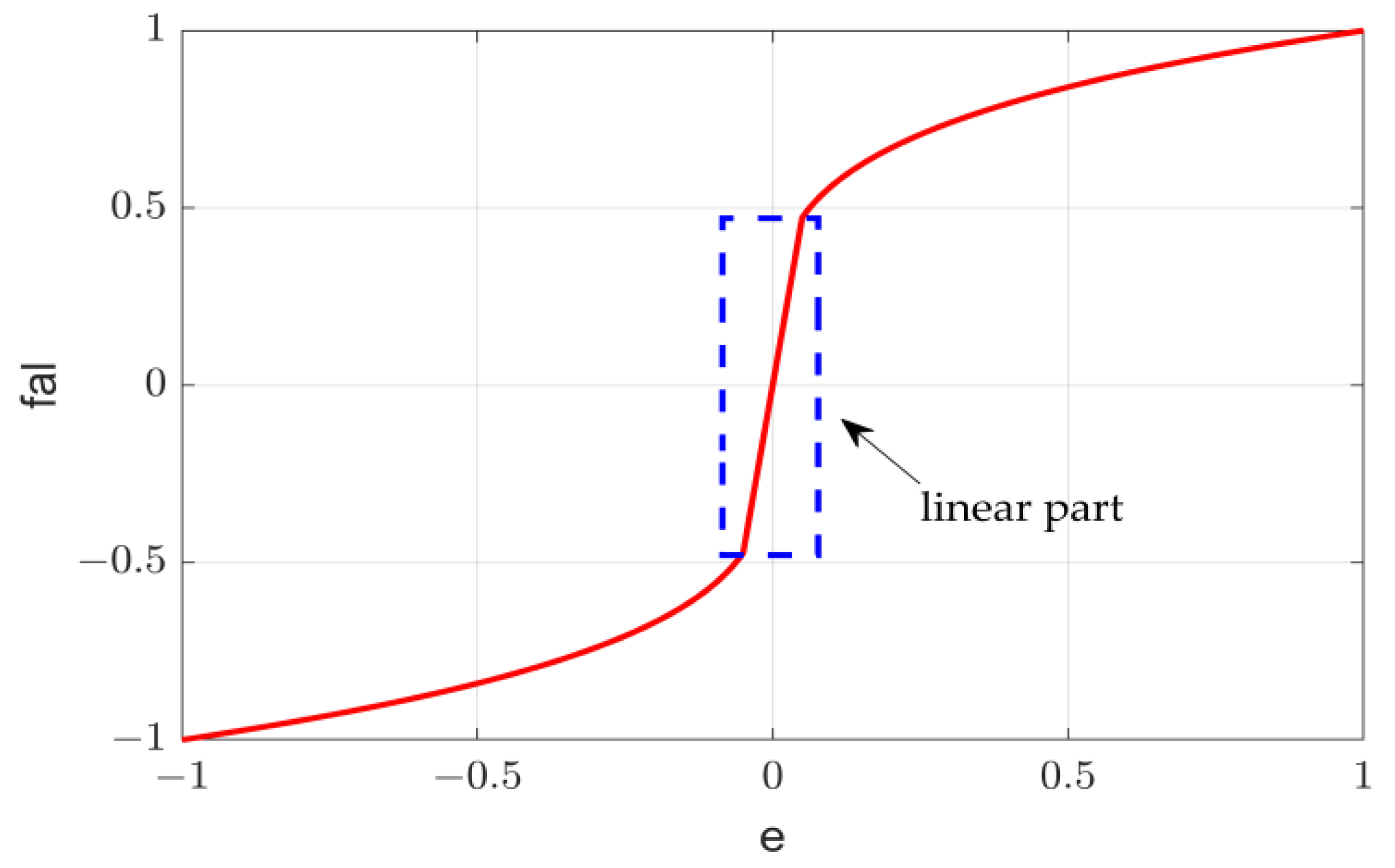
3.1. Nonlinear PI Cascade Controller

The cascade control can not only improve the control accuracy, stability, and anti-load interference ability of the system but also limit the maximum current during the motor starting and braking process, thereby improving the dynamic performance and steady-state performance of the control system. For nonlinear systems, the control effect of the classic PID controller is not good and is often accompanied by a certain amount of overshoot and following error and even oscillation. Introducing the nonlinear factors into the PID controller can link the gain parameters of the PID controller with the real-time error, thereby suppressing the influence of the nonlinear factors of the system on the control effect [40]. This paper uses a nonlinear combination of the PI form [41], which can be expressed as:

$$u_0={\beta }_{0}fal(e_0,\alpha ,\delta )+{\beta }_{1}fal(e_1,\alpha ,\delta ),$$

(4)

where ${\beta }_0$, ${\beta }_1$ are the control parameters; $e_0$, $e_1$ represent the error and the integral of the error, respectively; and $\alpha$, $\delta$ are the parameters that affect the smoothness and nonlinearity of the nonlinear function $fal(\cdot )$. The expression for $fal(\cdot )$ is:

$$fal(e,\alpha ,\delta )=\left\{\begin{array}{c}\frac{e}{{\delta }^{1-\alpha }}\hspace{1em}\hspace{1em}\left|e\right|\le \delta \hfill \\ {\left|e\right|}^{\alpha }\mathrm{sgn}(e)\left|e\right|>\delta \end{array}\right..$$

(5)

The changing law of $fal(\cdot )$ is shown in Figure 3. The nonlinear function $fal(\cdot )$ can indirectly adjust the control parameters of the controller according to the error and then suppress the high-frequency oscillation of the signal, which has the characteristics of strong adaptability [42].

In this study, a position–speed–current cascade control strategy was adopted, in which nonlinear PI control was adopted for both the speed loop and the current loop, and nonlinear P control was adopted for the position loop to obtain a good control effect. The control laws of the three loops are shown in Equation (6):

$$u_{p,s,c}=P_{p,s,c}fal(e_{p0,s0,c0},{\alpha }_{p0,s0,c0},{\delta }_{p0,s0,c0})+I_{s,c}fal(e_{p1,s1,c1},{\alpha }_{p1,s1,c1},{\delta }_{p1,s1,c1}).$$

(6)

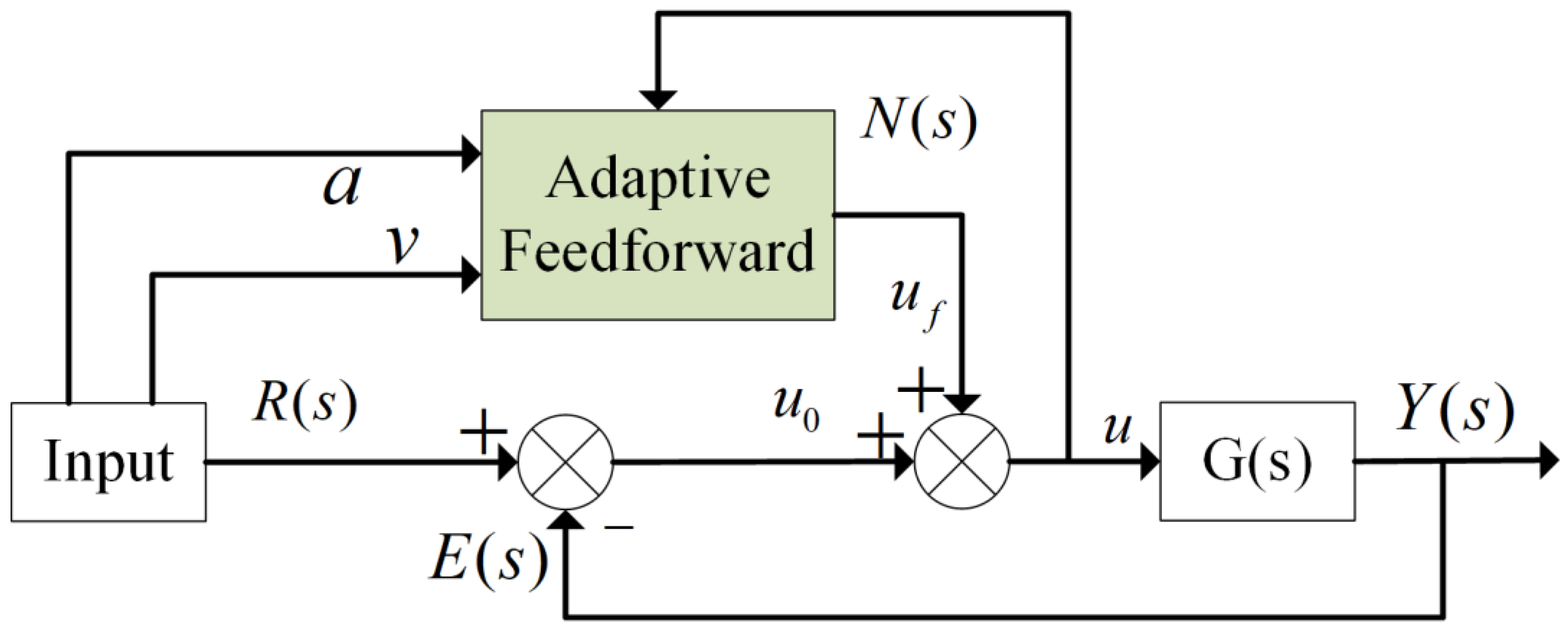
3.2. Adaptive Feedforward Compensator

In the control system, feedforward control can generate corresponding control quantities in time according to the change in the set value or external disturbance and add it to the system so that the controlled variable follows the set value or eliminates the influence of external disturbance. Figure 4 shows the schematic diagram of feedforward control.

From Figure 4, the relationship between output $Y(s)$ and input $R(s)$ of feedforward control can be obtained:

$$Y(s)=\frac{[1+N(s)]G(s)}{1+G(s)}R(s),$$

(7)

where $N(s)$ is the transfer function of the feedforward control, and $G(s)$ is the transfer function of the system combined with the feedback controller. The desired ideal system is one in which the output follows the input quickly and accurately: $Y(s)=R(s)$, at this time $N(s)=1/G(s)$. However, the actual model of the controlled object is complex and changeable, and a very accurate mathematical model cannot be obtained.

Therefore, this paper proposes an adaptive feedforward compensator, which can dynamically adjust the feedforward coefficient online based on feedback information, improve the adaptability of the feedforward compensator, and further improve the control accuracy of the system [43].

Speed feedforward control can reduce the following error of the control system caused by viscous resistance, and acceleration feedforward control can reduce the following error caused by inertia. Considering that the motion of the VCM is a motion with frequent acceleration and deceleration, a feedforward compensation algorithm that introduces speed and acceleration feedforward control was used in this study.

The output of the adaptive feedforward compensator can be expressed as:

$$u_f(t)=h(t)\theta (t),$$

(8)

where $h(t)={[v(t),a(t)]}^T$ is the system input matrix, and $\theta (t)={[K_v,K_a]}^T$ is the adaptive feedforward coefficient matrix. $v$ is the given speed, $a$ is the given acceleration, $K_v$ is the speed feedforward gain, and $K_a$ is the acceleration feedforward gain.

The system output after introducing the adaptive feedforward compensator can be expressed as:

$$u(t)=u_0(t)+u_f(t).$$

(9)

The estimated output of the adaptive feedforward compensator can be expressed as:

$${\widehat{u}}_f(t)=h(t)\widehat{\theta }(t),$$

(10)

where $\widehat{\theta }(t)$ is the estimated adaptive feedforward coefficient.

On the basis of the above formula, the recursive least squares (RLS) method was used to realize the adaptive online adjustment of the feedforward coefficient. The objective function was constructed, and the forgetting factor and damping factor were introduced:

$$\min J(\widehat{\theta }(t))={\displaystyle \sum _{k=1}^t{\lambda }^{t-k}}{[u(k)-h(k)\widehat{\theta }(k)]}^2+{\displaystyle \sum _{k=1}^t\mu }{[\widehat{\theta }(k)-\widehat{\theta }(k-1)]}^2,$$

(11)

where $\lambda$ is the forgetting factor. The smaller $\lambda$ is, the smaller the impact of old data on parameter estimation, but at the same time the more sensitive it is to noise. $\mu$ is the damping factor. Increasing the damping term can increase the stability of the algorithm. The RLS formula after introducing the forgetting factor and damping factor is:

$$\left\{\begin{array}{l}\widehat{\theta }(t)=\widehat{\theta }(t-1)+\lambda \mu P(t)[\widehat{\theta }(t)-\widehat{\theta }(t-1)]+P(t)h^T(t)[u(t)-h(t)\widehat{\theta }(t-1)]\hfill \\ P(t)={[\mu I-\lambda \mu I+\lambda P^{-1}(t-1)+h^T(t)h(t)]}^{-1}\hfill \end{array}\right.,$$

(12)

where $P(t)$ is the covariance of the estimation error, and $I$ is the identity matrix.

In the traditional RLS algorithm, the forgetting factor $\lambda$ is a fixed value, which makes it difficult to take into account the convergence speed and anti-interference ability of the algorithm. In order to solve the problem, this study involved the design of a dynamic forgetting factor: according to the system output error shown in Equation (13), the forgetting factor $\lambda (t)$ is dynamically adjusted, as shown in Equation (14).

$$\epsilon (t)=\left|u(t)-h(t)\widehat{\theta }(t-1)\right|.$$

(13)

$$\lambda (t)=\gamma +(1-\gamma )(1-erf(\beta \epsilon (t))),$$

(14)

where $\gamma$ and $\beta$ are variable parameters, and $\gamma$ usually takes $[0.9,1)$, and $\beta >0$. $erf(\cdot )$ is the Gaussian error function. The relationship between the forgetting factor and the system output error is shown in Figure 5.

It can be seen from Figure 5 that when $\epsilon (t)$ is large, $\lambda (t)$ is close to $\gamma$; when $\epsilon (t)$ is small, $\lambda (t)$ is close to 1. Dynamically adjusting the forgetting factor can balance the contradiction between the algorithm’s convergence speed and anti-interference ability.

3.3. Adaptive Feedforward–Nonlinear PI Cascade Composite Controller and Parameter Tuning

In this study, the adaptive feedforward compensator was introduced into the nonlinear PI cascade controller, and an adaptive feedforward–nonlinear PI cascade composite control strategy was constructed. The overall block diagram is shown in Figure 6. The overall control system includes curve planning, the adaptive feedforward compensator, and the nonlinear PI cascade controller. The adaptive feedforward compensator and the nonlinear PI cascade controller jointly complete the precise control of the VCM.

The AF-NLPI has many parameters, the conventional empirical tuning method is time-consuming and labor-intensive, and it is difficult to obtain optimal parameters, which affects the performance of the controller. To solve this problem, an optimization algorithm, the AOS algorithm [44], was adopted in this study to tune the control parameters.

The AOS algorithm is a new meta-heuristic optimization algorithm which is based on the atomic model of quantum mechanics. The algorithm simulates the configuration of electrons in the atomic model and regards the positions of electrons around the nucleus in the atomic model as candidate solutions and the energy level of electrons as the value of the objective function, and the candidate solutions with better objective function values represent the inner layers electrons with lower energy levels. The mathematical equation for the position of the electron in this algorithm can be expressed as:

$$X^k=\left[\begin{array}{l}{X}_1^k\hfill \\ X_2^k\hfill \\ ⋮\hfill \\ X_i^k\hfill \\ ⋮\hfill \\ X_p^k\hfill \end{array}\right]=\left[\begin{array}{llllll}{x}_1^1\hfill & x_1^2\hfill & \cdots \hfill & x_1^j\hfill & \cdots \hfill & x_1^d\hfill \\ x_2^1\hfill & x_2^2\hfill & \cdots \hfill & x_2^j\hfill & \cdots \hfill & x_2^d\hfill \\ ⋮\hfill & ⋮\hfill & \ddots \hfill & ⋮\hfill & \ddots \hfill & ⋮\hfill \\ x_i^1\hfill & x_i^2\hfill & \cdots \hfill & x_i^j\hfill & \cdots \hfill & x_i^d\hfill \\ ⋮\hfill & ⋮\hfill & \ddots \hfill & ⋮\hfill & \ddots \hfill & ⋮\hfill \\ x_p^1\hfill & x_p^2\hfill & \cdots \hfill & x_p^j\hfill & \cdots \hfill & x_p^d\hfill \end{array}\right],\left\{\begin{array}{c}i=1,2,\cdots ,p\\ j=1,2,\cdots ,d\\ k=1,2,\cdots ,n\end{array}\right.,$$

(15)

where $X_i^k$ is the i-th electron in the k-th virtual layer, $n$ is the maximum number of layers in the virtual layer, $p$ is the total number of electrons in the k-th virtual layer, and $d$ is the problem dimension representing the position of the electron.

The mathematical equation for the energy level of electrons in this algorithm can be expressed as:

$$E^k=\left[\begin{array}{l}{E}_1^k\hfill \\ E_2^k\hfill \\ ⋮\hfill \\ E_i^k\hfill \\ ⋮\hfill \\ E_p^k\hfill \end{array}\right],\left\{\begin{array}{c}i=1,2,\cdots ,p\\ k=1,2,\cdots ,n\end{array}\right.,$$

(16)

where $E_i^k$ represents the energy level of the i-th electron in the k-th virtual layer.

In each virtual layer, the candidate solution with the best objective function value is considered as the electron with the lowest energy level ($L{E}^k$). Further, the candidate solution with the best objective function value among all candidate solutions is regarded as the electron with the lowest energy level ($LE$) in the atom.

The binding state and binding energy of electrons in each virtual layer are determined by the average value of the positions of all electrons in the selected virtual layer and the value of the objective function, and the mathematical equation is as follows:

$$B{S}^k=\frac{{\displaystyle {\sum }_{i=1}^p{X}_i^k}}{p},$$

(17)

$$B{E}^k=\frac{{\displaystyle {\sum }_{i=1}^p{E}_i^k}}{p},$$

(18)

where $B{S}^k$ and $B{E}^k$ represent the binding state and binding energy of electrons in the k-th layer, respectively; $BS$ and $BE$ represent the binding state and binding energy of atoms, respectively.

In order to mathematically represent the effect of photons on the electrons surrounding the nucleus, a random number ($\varphi$) uniformly distributed between 0 and 1 is generated for each electron. The photon velocity ($PR$) is set to represent the probability that photons interact with electrons.

If $\varphi \ge PR$, the movement of electrons will be affected by photons: when $E_i^k\ge B{E}^k$, electrons tend to emit photons with ${\beta }_i$ and ${\gamma }_i$ energies; when $E_i^k<B{E}^k$, electrons tend to absorb photons with ${\beta }_i$ and ${\gamma }_i$ energies. If $\varphi <PR$, the movement of the electron will take into account some other action resulting in the absorption or emission of energy. In summary, the position update process of electrons is shown in Equation (19):

$$X_{i+1}^k=\left\{\begin{array}{l}{X}_i^k+{\alpha }_i\times ({\beta }_i\times LE-{\gamma }_i\times BS)/k,\varphi \ge PR \mathrm{and} E_i^k\ge B{E}^k \hfill \\ X_i^k+{\alpha }_i\times ({\beta }_i\times L{E}^k-{\gamma }_i\times B{S}^k),\varphi \ge PR \mathrm{and} E_i^k<B{E}^k\hfill \\ X_i^k+r_i,\hspace{1em}\hspace{1em}\hspace{1em}\hspace{1em}\hspace{1em}\hspace{1em}\hspace{1em}\hspace{1em}\hspace{1em}\varphi <PR\hfill \end{array}\right.,$$

(19)

where ${\alpha }_i$, ${\beta }_i$, ${\gamma }_i$, $r_i$ are randomly generated vectors uniformly distributed in the range (0, 1).

The AOS algorithm has achieved good results in dealing with mathematical and engineering design problems [45]. In this study, the AOS algorithm was selected to tune the parameters of the nonlinear PI cascade controller in order to obtain a good control effect. Through the AOS algorithm, the parameters of three NLPIs can be tuned simultaneously without having to adjust the parameters of the three NLPIs one by one, which improves the efficiency of parameter tuning. The principle is shown in Figure 7.

Integrated time and absolute error (ITAE) is an index to measure system performance. In this study, considering the following accuracy of the three loops comprehensively, Equation (20) was adopted as the fitness function:

$$ITA{E}_{sum}={\displaystyle {\int }_0^{t_1}t(w{(\left|e_p(t)\right| \left|e_s(t)\right| \left|e_i(t)\right|)}^{T}dt},$$

(20)

where $e_p(t)$ is the position error, $e_s(t)$ is the speed error, $e_i(t)$ is the current error, and $w$ is the weight matrix. The smaller the value of $ITA{E}_{sum}$ is, the better the achieved control performance index of the VCM. Thus, the ideal parameters can make the fitness function $ITA{E}_{sum}$ reach the minimum.

4. Simulation and Results Analysis

4.1. Parameter Setting and Model Building

The parameters of the VCM used in this study are shown in

Table 1. Parameters of the VCM.

Parameter Names and Symbols	Value
Resistance of energized coil  $R$	$3.8 \mathrm{\Omega }$
Inductance of energized coil  $L$	$1.0 \mathrm{m}\mathrm{H}$
Total mass of moving parts  $m$	$0.325 \mathrm{k}\mathrm{g}$
Damping coefficient  $c$	$4.2 \mathrm{N}\cdot \mathrm{s}\cdot {\mathrm{m}}^{-1}$
$\mathrm{Back} \mathrm{EMF} k_e$	$5.2 \mathrm{V}/\mathrm{m}/\mathrm{s}$
Elastic coefficient  $k$	$5.2 \mathrm{N}\cdot \mathrm{m}{\mathrm{m}}^{-1}$

:

Based on the above parameters, Saber and MAST languages were used in this study to model the VCM and driver and were combined with Simulink to build a control model in order to verify the effectiveness of the proposed controller more closely to reality, as shown in Figure 8. This study also involved the design of the classic PI cascade control model (PI), the nonlinear PI cascade control model (NLPI), and the nonlinear PI cascade control model with feedforward control (F-NLPI), and the controller proposed in this paper was compared with other methods to verify its better control performance.

In order to obtain ideal parameters, the nonlinear PI cascade controller uses the AOS algorithm to tune parameters. The nonlinear PI cascade controller has 11 parameters in total. In this study, the values of six of them were firstly set according to experience: ${\alpha }_p={\alpha }_s={\alpha }_c=0.75$, ${\delta }_p={\delta }_s={\delta }_c=0.005$, and the remaining parameters were tuned using the AOS algorithm. There are five parameters that need to be tuned: $P_p$, $P_s$, $P_c$, $I_s$, and $I_c$. Equation (20) was adopted as the fitness function. The parameter settings of the AOS algorithm are shown in

Table 2. Parameters of the AOS algorithm.

Parameter Name	Value
Number of electrons	50
Maximum number of layers	5
Foton rate	0.4
Dim	5
Max number of iterations	25
Upper limit	{30, 30, 100, 15, 40,000}
Lower limit	{1, 1, 1, 1, 10,000}
Weight matrix	{3, 10, 5}

.

In order to show the effectiveness of the selected AOS algorithm, this study also used the genetic algorithm (GA) and particle swarm optimization (PSO) algorithm to tune the parameters. The common parameters of the three algorithms were set to the same value; the crossover probability of GA was set to 0.9, and the mutation probability was set to 0.1. The self-best factor and global-best factor of PSO were both 1.5, and inertia weight was used.

Table 3. Parameters of the controller.

Parameter	${\mathit{P}}_{\mathit{p}}$	${\mathit{P}}_{\mathit{s}}$	${\mathit{I}}_{\mathit{s}}$	${\mathit{P}}_{\mathit{c}}$	${\mathit{I}}_{\mathit{c}}$
Value	16	6	60	11	30,000

shows the values of the parameters after the tuning is completed.

Figure 9 is the fitness function convergence curve of three algorithms. It can be seen that in the initial stage of the algorithm, the fitness function of the AOS algorithm drops rapidly, indicating that the algorithm has a good initial value optimization ability, and the search speed is fast. The algorithm reaches the minimum value in the 20th iteration and obtains ideal parameters, with a strong optimization ability.

By comparison, it was found from Figure 9 that the GA has poor search capabilities. The PSO algorithm has a weak search ability in the late iteration period and is prone to falling into local optimality. For the parameter tuning problem in this paper, the performance of the AOS algorithm is better than that of the GA and PSO algorithms.

4.2. Simulation Results and Analysis

This study first independently analyzed the effectiveness of the adaptive feedforward compensator and the nonlinear PI cascade controller proposed in this paper and analyzed the control performance of the composite controller by observing the following error. Then, the controller proposed in this paper was compared with NLPI and F-NLPI controllers to verify its good performance.

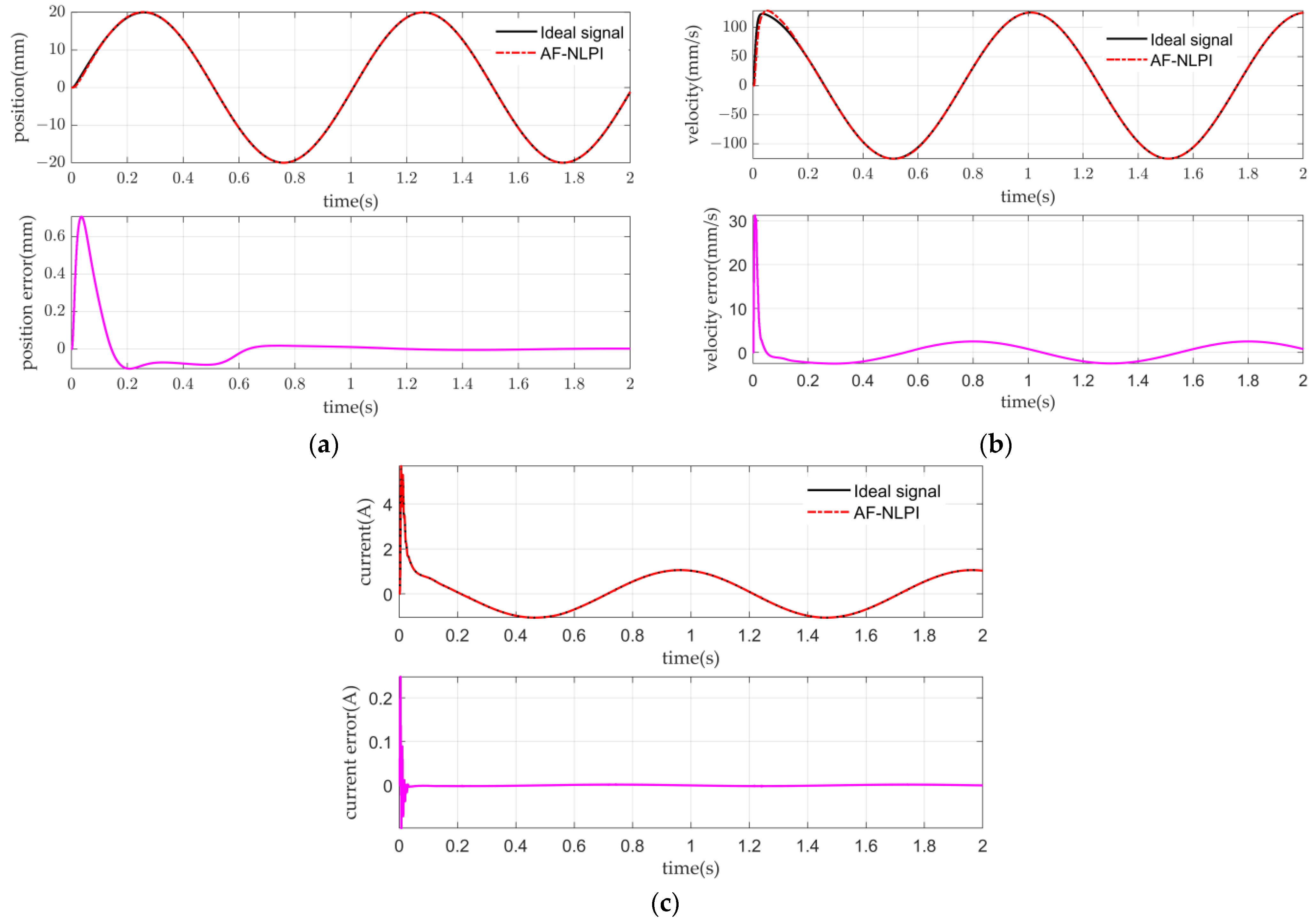
4.2.1. Performance of the Composite Controller

The parameters in Table 3 were used to simulate the system, and the input was set to a sine signal. First, the performance of nonlinear PI in improving control accuracy was verified. Figure 10 shows the following errors of the three loops of the two PI cascade controllers.

It can be seen from Figure 10 that the following errors of the three loops of the NLPI are smaller than those of the classical PI, and the response speed of the NLPI is similar to that of the classical PI. The dynamic performance and steady-state performance of the system are excellent, and the application of the nonlinear PI effectively solves the contradiction between the rapidity and stability of the control system.

Equation (21) is used as the control object to verify the performance of the proposed adaptive feedforward compensator. Comparing the improved RLS proposed in this paper with the classic RLS, other parameters of the control system remain consistent. The performance of the two algorithms when the system is affected by certain noise is shown in Figure 11. As can be seen from Figure 11, compared with the classic RLS, the adaptive feedforward compensator using IRLS has smaller following error.

$$G(s)=\frac{133}{s^2+25s}.$$

(21)

Figure 12 shows the change process of the feedforward coefficient. As can be seen from Figure 12, the convergence speed of the IRLS algorithm is similar to that of RLS, but it has excellent convergence speed and is not susceptible to noise interference. Overall, the proposed adaptive feedforward compensator has good performance.

The following and error curves of the controller for the position, speed, and current when the input is set to the planned motion trajectory are shown in Figure 13a, Figure 13b, and Figure 13c, respectively.

It can be seen from Figure 13a that, in the uniform motion segment, the following error of the controller to the position is less than 0.1 mm. It can be seen from Figure 13b that, in the stage of starting and reversing of the motor, the controller has a large error in following the speed curve. However, in the stage of uniform motion, the speed following error is less than 0.1 mm/s. The speed stability is excellent. It can be seen from Figure 13c that the controller responds to the current in a timely manner, and the following error is small, thus ensuring the response speed of the VCM.

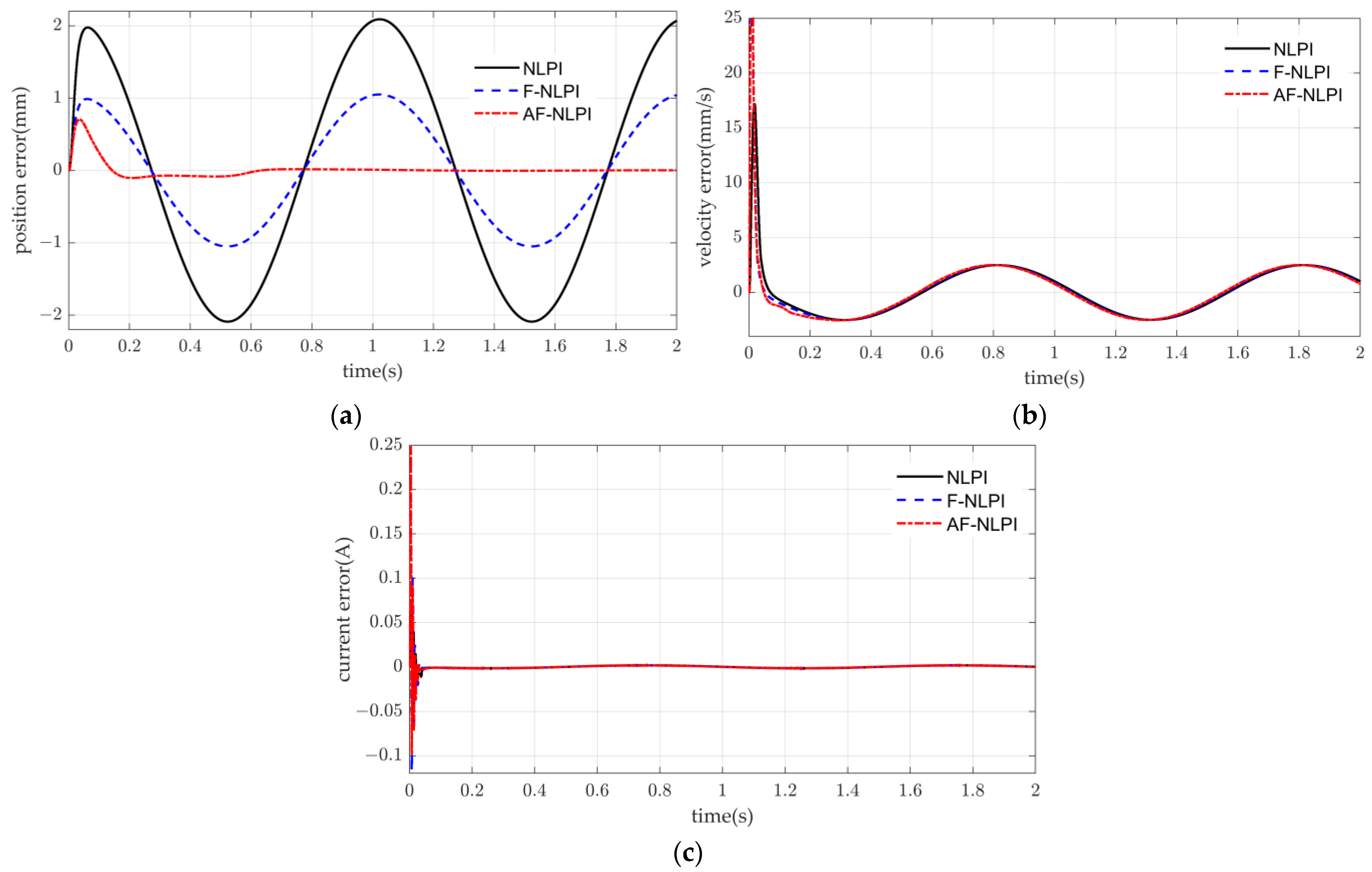
4.2.2. Comparison of Simulation Results for Different Controllers

The controller was simulated and compared with NLPI and F-NLPI controllers. The following errors of the three controllers were observed for position, speed, and current to verify the good performance of the controller proposed in this paper. Figure 14 shows the comparison of following errors of the three controllers. When the system is in the steady state, it can be seen from (b) and (c) in Figure 14 that the speed following error and current following error of the three controllers are very similar. However, it can be seen from Figure 14a, compared with controllers without feedforward control, that the position error of controllers with feedforward control is significantly reduced. Comparing the two controllers that introduce feedforward control, the adaptive feedback compensator used by the AF-NLPI has more adaptable compensation capabilities and reduces the position following error to close to zero.

Through the comparison of the NLPI and PI, it can be seen that the NLPI significantly reduces the following errors of the three loops and improves the following accuracy of the control system. After the introduction of the adaptive feedforward compensator proposed in this paper, the following performance of the VCM is effectively improved. Compared with the other three controllers, the AF-NLPI has the best performance on the following performance of the three loops, effectively improving the response speed and following accuracy of the VCM.

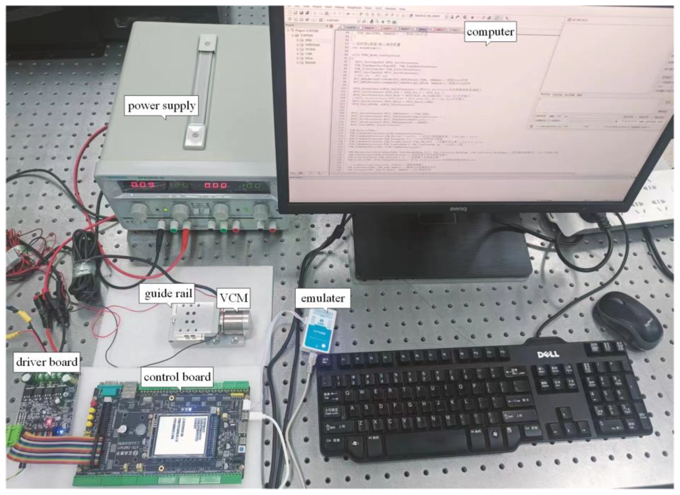
5. Experimental Verification

The motion form of the moving mirror includes acceleration motion, uniform motion, and deceleration motion. Frequent high-acceleration mutations may cause shocks, which is not conducive to the precise control of the control object [46]. Therefore, in this paper, the seventh-order S-curve is proposed to make the acceleration curve smooth and continuous and reduce the mechanical shock caused by acceleration changes [47]. The S-shaped curve in this paper is shown in Figure 15, which ensures the effective scanning displacement of the moving mirror while reducing the mechanical impact.

The experimental verification platform was built as shown in Figure 16. The actual control effect of the controller proposed in this paper on the optical path scanning control system was verified through experiments. The effective maximum displacement $\Delta zmax$ of the optical path scanning control system was set to 8 mm, the scanning speed $V$ to 10 mm/s, and the entire motion cycle to 1.6 s. The platform uses an industrial-grade motion controller STM32F407IG as the core controller, which outputs voltage signals to the DC drive board to drive the VCM. The experimental platform uses FACOR’s L series grating ruler as the position feedback sensor of the VCM, with an accuracy of $\pm 5 \mathrm{\mu }\mathrm{m}$.

Figure 17 is the actual measurement results of a motion cycle of the VCM. According to Figure 17a, in the stage of uniform motion, the position following error of the VCM is within 6.25 microns; only in the start-up and commutation stage is the following error relatively large. The position following performance is good. According to Figure 17b, the speed following effect of the VCM in the uniform motion stage is excellent. Intercepting the following error in the uniform motion stage, the standard deviation (STD) of speed fluctuation is 0.053. Figure 17c shows the current following curve of the VCM. Although there is a certain error, the overall following effect is good, and the response is timely.

Table 4. Position and speed following error.

Error	Maximum Error	Minimum Error	Average Error	STD of Error
$\mathrm{Position} (\mathrm{\mu }\mathrm{m}$)	6.25	0.00	1.95	1.40
$\mathrm{Speed} (\mathrm{m}\mathrm{m}/\mathrm{s}$)	0.30	0.00	0.07	0.05

shows the details of the position and velocity following errors in the uniform motion stage of the system. The maximum following errors of position and speed are 6.25 $\mathrm{\mu }\mathrm{m}$ and 0.30 $\mathrm{m}\mathrm{m}/\mathrm{s}$ respectively, and the STDs of errors are very small. The system’s following performance is excellent and stable.

The feasibility and effectiveness of the AF-NLPI proposed in this paper have been verified through experiments. The system is stable and has high following accuracy. The stability of the optical path scanning speed is 99.47%, which meets the requirement of the optical path scanning system.

6. Conclusions

Unstable optical path scanning motion affects the quality of the inverted spectrum. In order to improve the modulation quality of a portable FTS, an optical path scanning control system with a VCM as the control object was established. First, a nonlinear PI cascade controller was designed, and the parameters of controller were tuned using the AOS algorithm. Then, an adaptive feedforward compensator applying a dynamic forgetting factor was introduced. The feasibility and performance of the composite controller were verified through MATLAB and SABER joint simulation, and a physical experiment platform was built for testing.

The simulation results show that the AF-NLPI controller has excellent following performance for the planning curve, effectively reducing the following error of the position loop. The nonlinear PI effectively adjusts the contradiction between the rapidity and stability of the control system. Compared with the adaptive feedforward algorithm with a fixed forgetting factor, the adaptive feedforward algorithm using a dynamic forgetting factor has stronger overall performance. It has a good steady-state anti-interference ability and dynamic fast convergence ability. The experimental results show that, when the optical path scanning speed is set to 10 mm/s, the stability of the optical path scanning speed under the control of the AF-NLPI controller reaches 99.47%, which can meet the requirements of the optical path scanning control system in the actual FTS. The control strategy proposed in this paper has reference significance for the design of the optical path scanning control system of an FTS.

References

1. Sun, Y.; Yuan, M.; Liu, X.; Su, M.; Wang, L.; Zeng, Y.; Zang, H.; Nie, L. Comparative analysis of rapid quality evaluation of Salvia miltiorrhiza (Danshen) with Fourier transform near-infrared spectrometer and portable near-infrared spectrometer. Microchem. J. 2020, 159, 105492–105502. [Google Scholar] [CrossRef]
2. Jahromi, K.E.; Nematollahi, M.; Krebbers, R.; Abbas, M.A.; Khodabakhsh, A.; Harren, F.J.M. Fourier transform and grating-based spectroscopy with a mid-infrared supercontinuum source for trace gas detection in fruit quality monitoring. Opt. Express 2021, 29, 12381–12397. [Google Scholar] [CrossRef]
3. Luo, S.; Tian, J.; Liu, Z.; Lu, Q.; Zhong, K.; Yang, X. Rapid determination of styrene-butadiene-styrene (SBS) content in modified asphalt based on Fourier transform infrared (FTIR) spectrometer and linear regression analysis. Measurement 2020, 151, 107204–107212. [Google Scholar] [CrossRef]
4. Wang, R.; Dong, D.; Ye, S.; Jiao, L. Measurement of Volatile Compounds Released from Plastic Using Long-Optical-Path FTIR. Spectrosc. Spectr. Anal. 2021, 41, 3039–3044. [Google Scholar]
5. Cui, F.X.; Hao, Y.; Ma, F.X.; Wu, J.; Wang, A.; Li, D.; Li, Y.Y. Optimization of FTIR Passive Remote Sensing Signal-to-Noise Ratio and Its Application in SF6, Leak Detection in Transform Substation. Spectrosc. Spectr. Anal. 2021, 41, 1436–1440. [Google Scholar]
6. Pan, M.; Sun, S.; Zhou, Q.; Chen, J. A Simple and Portable Screening Method for Adulterated Olive Oils Using the Hand-Held FTIR Spectrometer and Chemometrics Tools. J. Food Sci. 2018, 83, 1605–1612. [Google Scholar] [CrossRef]
7. Cebi, N.; Bekiroglu, H.; Erarslan, A.; Rodriguez-Saona, L. Rapid Sensing: Hand-Held and Portable FTIR Applications for On-Site Food Quality Control from Farm to Fork. Molecules 2023, 28, 3727–3741. [Google Scholar] [CrossRef] [PubMed]
8. Deng, Y.; Xu, L.; Sheng, X.; Sun, Y.; Xu, H.; Xu, H.; Wu, H. Vehicle-Mounted Solar Occultation Flux Fourier Transform Infrared Spectrometer and Its Remote Sensing Application. Sensors 2023, 23, 4317–4334. [Google Scholar] [CrossRef]
9. Qu, L.; Xu, L.; Liu, J.; Feng, M.; Liu, W.; Xu, H.; Jin, L. Numerical Simulation Analysis of Portable High-Speed FTIR Rotary Interferometers. Acta Opt. Sin. 2021, 41, 0907001. [Google Scholar]
10. Zhang, M.; Zhang, J.; Yang, H. Research on speed stability of moving mirror in FTIR spectrometer. Infrared Laser Eng. 2014, 43, 1240–1246. [Google Scholar]
11. Qin, Y.; Li, X.; Han, X.; Tong, J.; Gao, M.; Liu, S. Study on the influence of interferometer velocity fluctuation on spectral signal-to-noise ratio. J. Optoelectron. Laser 2022, 33, 0449–0457. [Google Scholar] [CrossRef]
12. Gao, H.; Zhang, F.; Wang, E.; Liu, B.; Zeng, W.; Wang, Z. Optimization and simulation of a voice coil motor for fuel injectors of two-stroke aviation piston engine. Adv. Mech. Eng. 2019, 11, 1–17. [Google Scholar] [CrossRef]
13. Koerner, L.J.; Secord, T.W. An embedded electrical impedance analyzer based on the AD5933 for the determination of voice coil motor mechanical properties. Sens. Actuators A Phys. 2019, 295, 99–112. [Google Scholar] [CrossRef]
14. Rosier, A.; Mabo, P.; Chauvin, M.; Burgun, A. An Ontology-Based Annotation of Cardiac Implantable Electronic Devices to Detect Therapy Changes in a National Registry. IEEE J. Biomed. Health Inform. 2015, 19, 971–978. [Google Scholar] [CrossRef] [PubMed]
15. Qu, L. Research on Key Technology and Application of Portable FTIR Spectrometer. Ph.D. Dissertation, University of Science and Technology of China, Anhui, China, 2021. [Google Scholar]
16. Shi, L.; Liu, J.; Gao, W.; Zhang, Q.-X.; Wang, W. Design of a Moving Mirror Scanning System in Fourier Transform Infrared Spectrometer. Acta Photonica Sin. 2015, 44, 0430002–0430007. [Google Scholar] [CrossRef]
17. Ren, L.; Yang, H.; Wei, H.; Li, Y. Design for multi-gases analyzer based on FTIR principle. Infrared Laser Eng. 2013, 42, 3175–3179. [Google Scholar]
18. Wang, W.; Lu, Y.; Lu, F.; Zhang, T.; Fu, Y. Design of moving mirror control system of Fourier transform infrared spectrometer based on DSP. Chin. J. Quantum Electron. 2015, 32, 8. [Google Scholar]
19. Liu, R.-L.; Yin, D.-K. Driving Control Technology for Moving Mirror of Fourier Transform Spectrometer. Infrared 2009, 30, 20–25. [Google Scholar]
20. Liang, X.-W.; Shi, L. Design of a Moving Mirror Scanning System for Portable Interferometer. Spectrosc. Spectr. Anal. 2017, 37, 3255–3259. [Google Scholar]
21. Li, Z.B.; Xu, X.; Le, Y.; Xu, F.Q.; Li, J.-W. Motion Control of Moving Mirror Based on Fixed-Mirror Adjustment in FTIR Spectrometer. Spectrosc. Spectr. Anal. 2012, 32, 2295–2298. [Google Scholar]
22. Guo, L.; Ma, W.; Wang, C.; Lin, Z.; Wang, H. Design of translating optical path scanning control system for Fourier spectrometer. Infrared Laser Eng. 2020, 49, 0105002. [Google Scholar]
23. Guo, L.; Wang, H.; Wang, C.; Ma, W.; Zhe, L. Optical Path Scanning Control System Based on Modified Repetitive Control. Spacecr. Recovery Remote Sens. 2019, 40, 32–40. [Google Scholar] [CrossRef]
24. Li, T.; Hua, J.-W.; Xia, X.; Sheng, H. Simulation of Moving Mirror Control in Fourier Transform Spectrometer. Meas. Control Technol. 2014, 33, 111–114. [Google Scholar]
25. Shi, Y.; Zhou, C.; Yin, Q.; Zhou, Y. Simulation on Interference Control System in Fourier Transform Spectrograph. J. Syst. Simul. 2013, 25, 753–759. [Google Scholar] [CrossRef]
26. Zhou, X.; Gao, H.; Zhao, B.; Zhao, L. A GA-based parameters tuning method for an ADRC controller of ISP for aerial remote sensing applications. ISA Trans. 2018, 81, 318–328. [Google Scholar] [CrossRef]
27. Luo, Y.; Chen, Y.Q.; Wang, C.Y.; Pi, Y.G. Tuning fractional order proportional integral controllers for fractional order systems. J. Process Control 2010, 20, 823–831. [Google Scholar] [CrossRef]
28. Yang, J.; Ren, Y. Application of fractional compound control in photoelectric stable platform. Electron. Opt. Control. 2020, 27, 73–78. [Google Scholar]
29. Saxena, S.; Hote, Y.V. Design and Validation of Fractional-Order Control Scheme for DC Servomotor via Internal Model Control Approach. IETE Tech. Rev. 2017, 36, 49–60. [Google Scholar] [CrossRef]
30. Meng, F.; Liu, S.; Liu, K. Design of an Optimal Fractional Order PID for Constant Tension Control System. IEEE Access 2020, 8, 58933–58939. [Google Scholar] [CrossRef]
31. Konstantopoulos, G.C.; Baldivieso-Monasterios, P.R. State-limiting PID controller for a class of nonlinear systems with constant uncertainties. Int. J. Robust Nonlinear Control. 2019, 30, 1770–1787. [Google Scholar] [CrossRef]
32. Cheng, M.; Zhai, P.; Zhang, Y.; Li, J.; Feng, K. A Voice Coil Motor-Driven Precision Positioning System Based on Self-Learning Nonlinear PID. Trans. China Electrotech. Soc. 2023, 38, 1519–1570. [Google Scholar] [CrossRef]
33. Fonseca, R.R.; Sencio, R.R.; Franco, I.C.; Da Silva, F.V. An Adaptive Fuzzy Feedforward-Feedback Control System Applied to a Saccharification Process. Chem. Prod. Process Model. 2018, 13, 12. [Google Scholar] [CrossRef]
34. Cui, J.; Wang, S.; Chu, Z.Y. Feed-forward compensation control of nonlinear friction for high acceleration motion system. Opt. Precis. Eng. 2018, 26, 0077–0085. [Google Scholar]
35. Yang, H.; Wu, Q.-Z.; Fan, Y.-K.; Li, Y.-P. Application Research of Acceleration Feedforward in the High Precision Servo Tracking System. Electro-Opt. Technol. Appl. 2007, 22, 0048–0051. [Google Scholar]
36. Li, W.; Hou, B.; Gao, J.; Wang, S. Compound Feedforward Control of Velocity Plus Acceleration for Linear Motor. Mach. Tool Hydraul. 2015, 43, 146–149. [Google Scholar]
37. Yang, K. Research and Application on a Certain Number of Core Technologies of Fourier Transform Infrared Spectrometer. Ph.D. Dissertation, Wuhan University, Wuhan, China, 2010. [Google Scholar]
38. Hsu, C.-F.; Wong, K.-Y. On-line constructive fuzzy sliding-mode control for voice coil motors. Appl. Soft Comput. 2016, 47, 415–423. [Google Scholar] [CrossRef]
39. Chen, Q.; Li, L.; Wang, M.; Pei, L. The precise modeling and active disturbance rejection control of voice coil motor in high precision motion control system. Appl. Math. Model. 2015, 39, 5936–5948. [Google Scholar] [CrossRef]
40. Li, Z.-h.; Chen, G.; Zhou, L. ADRC Algorithm for Position Control of Voice Coil Motor. J. Nanjing Inst. Technol. (Nat. Sci. Ed.) 2019, 17, 25–30. [Google Scholar]
41. Wei, W.; Zhao, X. Fast Steering Mirror Control Based on Improved Active Disturbance Rejection. Infrared Technol. 2018, 40, 1071–1076. [Google Scholar]
42. Li, W.-B.; Tian, D. A Three-closed-loop Feedward PID Servo Controller Based on S-curve. Technol. IoT AI 2021, 4, 021–029. [Google Scholar]
43. Tan, E.; Shi, T.; Zhang, Z.; Zhang, L. Adaptive Feedforward Control for Reticle Stage of Lithography. Control Eng. China 2021, 28, 1069–1074. [Google Scholar]
44. Azizi, M. Atomic orbital search: A novel metaheuristic algorithm. Appl. Math. Model. 2021, 93, 657–683. [Google Scholar] [CrossRef]
45. Azizi, M.; Talatahari, S.; Giaralis, A. Optimization of Engineering Design Problems Using Atomic Orbital Search Algorithm. IEEE Access 2021, 9, 102497–102519. [Google Scholar] [CrossRef]
46. Li, L.-H.; Zhang, Z.-Q.; Guo, Z.; Luo, Y.-Y.; Zhou, L.-Q.; Yao, J. Optimal order polynomial motion profile for high-precision flexible scanning platform. Opt. Precis. Eng. 2021, 29, 2400–2411. [Google Scholar] [CrossRef]
47. Nguyen, K.D.; Ng, T.-C.; Chen, I.-M. On Algorithms for Planning S-Curve Motion Profiles. Int. J. Adv. Robot. Syst. 2008, 5, 99–106. [Google Scholar] [CrossRef]
Figure 1. Michelson interferometer using cube corner.
Actuators 13 00035 g001
Figure 2. Equivalent model of a VCM: (a) electrical model and (b) mechanical model.
Actuators 13 00035 g002
Figure 3. Function change curve.
Actuators 13 00035 g003
Figure 4. Block diagram of adaptive feedforward compensator.
Actuators 13 00035 g004
Figure 5. Dynamic adjustment of the forgetting factor.
Actuators 13 00035 g005
Figure 6. Overall block diagram of the control system.
Actuators 13 00035 g006
Figure 7. Block diagram of parameter tuning with AOS algorithm.
Actuators 13 00035 g007
Figure 8. Optical path scanning control system built with Saber and Simulink.
Actuators 13 00035 g008
Figure 9. Convergence curve of the fitness function.
Actuators 13 00035 g009
Figure 10. The following error of the two PI cascade controllers: (a) position following error; (b) speed following error; (c) current following error.
Actuators 13 00035 g010
Figure 11. Control effects of two adaptive feedforward compensators.
Actuators 13 00035 g011
Figure 12. Changes in feedforward coefficient.
Actuators 13 00035 g012
Figure 13. The performance of the composite controller: (a) position following curve and following error; (b) speed following curve and following error; (c) current following curve and following error.
Actuators 13 00035 g013
Figure 14. Following error curves for three controllers: (a) position following error; (b) speed following error; (c) current following error.
Actuators 13 00035 g014
Figure 15. Position and speed curves based on S-curve planning.
Actuators 13 00035 g015
Figure 16. Physical experiment verification platform.
Actuators 13 00035 g016
Figure 17. Experimental following curves and error curves of the VCM: (a) position following curve and following error; (b) speed following curve and following error; (c) current following curve.
Actuators 13 00035 g017