Internal Model Principle-Based Extended State Observer for the Uncertain Systems with Nonconstant Disturbances

Abstract

Existing traditional expansion state observers exhibit good tracking performance for constant and low-frequency disturbances. However, their ability to track non-constant disturbances such as ramp and high-frequency harmonics is inadequate. This paper proposes an extended state observer design method based on the internal model principle. This method achieves precise tracking of non-constant disturbances in the system, effectively addressing the issue of disturbance estimation errors in conventional expansion state observers. When applied to control systems, this approach significantly mitigates or suppresses system vibrations caused by non-constant disturbances, thereby enhancing control accuracy. Furthermore, it demonstrates the stability of the controlled system and the active disturbance rejection controller parameters over a wide range of variations. Simulation results indicate that the ADRC controller based on the proposed observer in this paper offers notable advantages, including high tracking accuracy, strong disturbance rejection capability, and good stability, leading to commendable control performance.

1. Introduction

Industrial systems often encounter non-constant external disturbances, which can adversely affect control performance. Various control methods have been proposed to mitigate disturbances and maintain desired control performance [1,2,3,4]. These include Active Disturbance Rejection Control (ADRC) [1], control based on disturbance observers [2], equivalent input disturbance methods [3], and control based on uncertainty and disturbance estimation (UDE) [4]. ADRC has gained popularity due to its ability to achieve precise control with minimal information about the controlled object, and it has been successfully applied in numerous control systems [5,6,7,8,9].

ADRC is a nonlinear control inherited from PID proposed by Jingqing Han from the Chinese Academy of Sciences [10]. Subsequently, Professor Zhiqiang Gao of Cleveland State University in the United States proposed Linear Active Disturbance Rejection Control (LADRC) and its parameter tuning method, introducing the concepts of observer bandwidth and controller bandwidth for LADRC design [11]. The Expansion State Observer (ESO), as a core component of ADRC control technology, has also been widely utilized [12,13,14,15,16]. ESO treats the model mismatch (uncertainty) and external disturbances as new states in the system and extends the state space to observe these new system states, thereby estimating the total disturbance [17]. However, traditional ESO, being equivalent to an integral controller, exhibits excellent tracking performance for constant or slowly changing disturbances, but often falls short in tracking rapidly changing disturbances [18]. As mentioned in reference [19], the conventional ESO can estimate unknown disturbances very well only when the disturbances consist of low-frequency components. On one hand, the model-free characteristic of ESO leads to strong robustness against uncertainty and disturbance; however, on the other hand, it may somewhat waste information about disturbances that are known to us. In existing observers such as sliding mode observers [20] and expanded high-gain observers [21,22], there is also some waste of known information. In reality, in engineering applications, we are not completely unaware of disturbance information, such as smoothness, boundedness and dynamic information about disturbances. In reference [23], it is mentioned that in large-scale wind turbine systems, the rotational frequency of the wind rotor is three times the disturbance frequency experienced by the wind turbine. Additionally, mechanical resonance issues commonly occur in servo systems, and online detection techniques for resonance frequencies have become quite mature. For instance, in reference [24], the second-order generalized integrator-frequency-locked loop is employed for online detection of resonance frequencies. This information is very useful for control. A typical example is harmonic disturbance where the known frequencies are highly useful for the internal model principle (IMP), which is an elegant approach to robust output regulation [25], yet this information is entirely wasted in ADRC.

Regarding the above issues, this paper proposes an IMP-ESO (internal model principle-based expanded state observer), which maximally utilizes interference information by studying the characteristics of disturbance signals based on the idea of expanded state observation and combining with the internal model principle. The internal model principle (IMP) indicates that any controller must include the internal model and disturbance model characteristics of the controlled system to achieve optimal performance. This means that the controller must be able to accurately establish the behavioral model of the controlled system, including its dynamics and response characteristics, in order to make effective control decisions.

Utilizing the spectral characteristics of the total disturbance, the difference between the estimated system state and the actual state is input into the proposed disturbance tracker based on the internal model principle, generating a disturbance-tracking signal. The IMP-ESO presented in this paper effectively tracks non-constant disturbances, enabling control systems utilizing IMP-ESO to effectively suppress disturbances and improve control accuracy, response speed, and disturbance rejection capability. Finally, the effectiveness of the proposed method is validated through simulations on a second-order control system.

The main contributions of this paper are as follows:

• Introduction of a design concept and methodology for an internal model principle-based ESO tailored to different types of disturbances, providing a novel approach to Active Disturbance Rejection Control (ADRC) that effectively suppresses non-constant disturbances.
• Further extension and improvement of the ESO by proposing a new disturbance-tracking paradigm.
• Theoretical analysis and simulation results indicate that the internal model principle-based extended state observer (IMP-ESO-ADRC) possesses several advantages, including high tracking accuracy, strong disturbance rejection capability, and good stability. This controller exhibits robustness in the face of disturbances and showcases a remarkable ability to mitigate their effects. The remaining sections of this paper are organized as follows:

Section 2 discusses the limitations of traditional ESO.

Section 3 introduces the design methodology of IMP-ESO and provides parameter tuning methods.

Section 4 presents the frequency domain analysis and simulation of IMP-ESO.

Section 5 presents the simulated results, which offer a comprehensive evaluation of the proposed IMP-ESO-ADRC.

Finally, Section 6 concludes the paper.

2. Expansion State Observer

Firstly, consider the following n-th order linear system: (1):

$$\{\begin{array}{l}{\dot{x}}_1(t)=x_2(t)\\ {\dot{x}}_2(t)=x_3(t)\\ \hspace{1em}\hspace{1em}⋮\\ {\dot{x}}_{n-1}(t)=x_n(t)\\ {\dot{x}}_n(t)=f(t)+bu(t)\\ y(t)=x_1(t)\end{array}\hspace{1em}$$

(1)

where $x_1(t)$, $x_2(t)$, … and $x_n(t)$ represent the system state variables, $u(t)$ denotes the control input, $y(t)$ signifies the control output, $f(t)$ is a function containing external disturbances to the system and undocumented system dynamics, and $b$ is the input gain.

According to Formula (1), the expanded state equation corresponding to an n-order system can be obtained as:

$$\{\begin{array}{l}{\dot{x}}_1(t)=x_2(t)\\ {\dot{x}}_2(t)=x_3(t)\\ \hspace{1em}\hspace{1em}⋮\\ {\dot{x}}_{n-1}(t)=x_n(t)\\ {\dot{x}}_n(t)=x_{n+1}(t)+\overline{b}u(t)\\ y(t)=x_1(t)\end{array}\hspace{1em}$$

(2)

In this regard, $x_{n+1}(t)=f(t)+(b-\overline{b})u(t)$ is the expansion state, $\overline{b}$ representing the nominal gain of the system. Accordingly, the conventional state observer (ESO) [18] corresponding to this n-th order system is as follows:

$$\{\begin{array}{l}{\dot{\widehat{x}}}_1(t)={\widehat{x}}_2(t)+{\beta }_1(x_1(t)-{\widehat{x}}_1(t))\\ {\dot{\widehat{x}}}_2(t)={\widehat{x}}_3(t)+{\beta }_2(x_1(t)-{\widehat{x}}_1(t))\\ \hspace{1em}\hspace{1em}⋮\\ {\dot{\widehat{x}}}_{n-1}(t)={\widehat{x}}_n(t)+{\beta }_{n-1}(x_1(t)-{\widehat{x}}_1(t))\\ {\dot{\widehat{x}}}_n(t)={\widehat{x}}_{n+1}(t)+{\beta }_n(x_1(t)-{\widehat{x}}_1(t))+\overline{b}u(t)\\ {\dot{\widehat{x}}}_{n+1}(t)={\beta }_{n+1}(x_1(t)-{\widehat{x}}_1(t))\\ \widehat{y}(t)={\widehat{x}}_1(t)\end{array}$$

(3)

where ${\widehat{x}}_1(t)$, ${\widehat{x}}_2(t)$, …, ${\widehat{x}}_{n+1}(t)$ respectively represent the estimated state variables for the system state variables $x_1(t)$, $x_2(t)$, …, $x_{n+1}(t)$. $u(t)$ denotes the control input, and $\widehat{y}(t)$ signifies the estimated control output. ${\widehat{x}}_{n+1}(t)$ represents the total disturbance estimation for the conventional ESO, and $\overline{b}$ is the input gain. ${\beta }_1$, ${\beta }_2$, …, ${\beta }_{n+1}$ are the gain of the ESO.

As shown in Figure 1, the classic second-order ADRC system consists of:

Where $k_1$ and $k_2$ represent feedback gain, with ${\widehat{x}}_1(t)$ and ${\widehat{x}}_2(t)$, respectively, denoting estimated state variables corresponding to the system state variables $x_1(t)$ and $x_2(t)$; $r(t)$ is the input signal, $u(t)$ indicates the control input, $\overline{b}$ is the input gain, and $y(t)=x_1(t)$.

As evident from Equation (3), the traditional ESO utilizes ${\dot{\widehat{x}}}_3(t)={\beta }_3(x_1(t)-{\widehat{x}}_1(t))$ as the total disturbance estimation for the ADRC system, as shown in Figure 1.

Hence, it is evident that the traditional ESO algorithm can only estimate the error better when the disturbance is of low frequency. Furthermore, from the theoretical research on traditional ESO presented in reference [19], it is known that traditional ESO exhibits good tracking performance only for constant and low-frequency disturbances. When it comes to high-frequency disturbances, especially harmonic disturbances, there are significant tracking errors and considerable phase lag, resulting in low control accuracy in the closed-loop system. In practical applications where non-constant disturbances are present, the traditional ESO often fails to accurately estimate the total disturbance of the system.

3. Controller Design and Stability Analysis

3.1. Controller Design

In response to the issues raised in the previous section, this paper proposes the following improvements.

From the principles of internal model principle, it is evident that a feedback controller must incorporate the spectral characteristics of external disturbances in order to enable the closed-loop system to resist disturbances, model mismatches, and regulate the output. Similarly, the internal model principle can be applied to redesign the ESO in the disturbance observation loop. This new design, known as the IMP-ESO, can accurately track the total disturbance of the system in real-time and achieve error-free tracking.

Considering the application of the internal model principle, the expansion state equation for the IMP-ESO can be expressed as follows:

$$\{\begin{array}{l}{\dot{\widehat{x}}}_1(t)={\widehat{x}}_2(t)+{\beta }_1(x_1(t)-{\widehat{x}}_1(t))\\ {\dot{\widehat{x}}}_2(t)={\widehat{x}}_3(t)+{\beta }_2(x_1(t)-{\widehat{x}}_1(t))\\ \hspace{1em}\hspace{1em}⋮\\ {\dot{\widehat{x}}}_{n-1}(t)={\widehat{x}}_n(t)+{\beta }_{n-1}(x_1(t)-{\widehat{x}}_1(t))\\ {\dot{\widehat{x}}}_n(t)={\widehat{x}}_{n+1}(t)+{\beta }_n(x_1(t)-{\widehat{x}}_1(t))+\overline{b}u(t)\\ {\dot{\widehat{x}}}_{n+1}(t)=G_z(t)(x_1(t)-{\widehat{x}}_1(t))\\ \widehat{y}(t)={\widehat{x}}_1(t)\end{array}$$

(4)

where ${\widehat{x}}_1(t)$, ${\widehat{x}}_2(t)$, …,${\widehat{x}}_{n+1}(t)$ represent the estimated state variables for the system states $x_1(t)$, $x_2(t)$, …, $x_{n+1}(t)$, respectively. ${\widehat{x}}_{n+1}(t)$ denotes the total disturbance estimation, while ${\beta }_1$, ${\beta }_2$, …, ${\beta }_{n+1}$ correspond to the gain of the IMP-ESO. After Laplace transform, $G_z(t)$ can obtain $G_z(s)$. $G_z(s)$ represents the transfer function constructed based on the internal model principle. $u(t)$ denotes the control input, $\widehat{y}(t)$ signifies the control output, and $\overline{b}$ denotes the input gain.

To facilitate formula derivation and exposition, let us transform the variable state space into the error state space, by introducing the following notation:

$$\{\begin{array}{l}{e}_1(t)=x_1(t)-{\widehat{x}}_1(t)\\ e_2(t)=x_2(t)-{\widehat{x}}_2(t)\\ \hspace{1em}\hspace{1em}⋮\\ e_{n-1}(t)=x_{n-1}(t)-{\widehat{x}}_{n-1}(t)\\ e_n(t)=x_n(t)-{\widehat{x}}_n(t)\\ e_{n+1}(t)=x_{n+1}(t)-{\widehat{x}}_{n+1}(t)\end{array}$$

(5)

Therefore, combining Equations (1) and (5), we can derive the following expressions:

$$\{\begin{array}{l}{\dot{e}}_1(t)=e_2(t)-{\beta }_1{e}_1(t)\\ {\dot{e}}_2(t)=e_3(t)-{\beta }_2{e}_1(t)\\ \hspace{1em}\hspace{1em}⋮\\ {\dot{e}}_{n-1}(t)=e_n(t)-{\beta }_{n-1}{e}_1(t)\\ {\dot{e}}_n(t)=e_{n+1}(t)-{\beta }_n{e}_1(t)\\ {\dot{\widehat{x}}}_{n+1}(t)=G_z(t)e_1(t)\end{array}$$

(6)

From Equation (6), we can obtain its transfer function as follows:

$$\{\begin{array}{l}s{E}_1(s)=E_2(s)-{\beta }_1{E}_1(s)\\ s{E}_2(s)=E_3(s)-{\beta }_2{E}_1(s)\\ \hspace{1em}\hspace{1em}⋮\\ s{E}_{n-1}(s)=E_n(s)-{\beta }_{n-1}{E}_1(s)\\ s{E}_n(s)=E_{n+1}(s)-{\beta }_n{E}_1(s)\\ s{\widehat{X}}_{n+1}(s)=G_z(s)E_1(s)\end{array}$$

(7)

By integrating Equation (4) into Equation (7), we can derive the following expression:

$$\{\begin{array}{l}{E}_1(s)=\frac{1}{{\beta }_n+{\beta }_{n-1}s+\cdots +{\beta }_2{s}^{n-2}+{\beta }_1{s}^{n-1}+s^n}{E}_{n+1}(s)\\ E_{n+1}(s)=X_{n+1}(s)-{\widehat{X}}_{n+1}(s)\\ s{\widehat{X}}_{n+1}(s)=G_z(s)E_1(s)\end{array}$$

(8)

Simplifying Equation (8), we can rearrange it to obtain:

$$E_{n+1}(s)=X_{n+1}(s)-{\widehat{X}}_{n+1}(s)=\left(\frac{{\beta }_n+{\beta }_{n-1}s+\cdots +{\beta }_2{s}^{n-2}+{\beta }_1{s}^{n-1}+s^n}{{\beta }_n+{\beta }_{n-1}s+\cdots +{\beta }_2{s}^{n-2}+{\beta }_1{s}^{n-1}+s^n+\frac{G_z(s)}{s}}\right)X_{n+1}(s)$$

(9)

Therefore, by ensuring that the pole distribution of the characteristic polynomial in Equation (11) lies in the left half plane, we can satisfy the stability requirements of the system. This allows us to obtain the disturbance tracking transfer function under different disturbance characteristics and determine the appropriate observer parameter values.

Assuming that the disturbance signal is a harmonic signal, i.e., $X_3(s)=\frac{{{\omega }_n}^2}{s^2+{{\omega }_n}^2}$, we can use the pole placement method to determine the observer poles:

$$\{\begin{array}{l}{\beta }_1=5{\omega }_0\\ {\beta }_2=9{{\omega }_0}^2-{{\omega }_n}^2\\ G_z(s)=\frac{(9{{\omega }_0}^3-5{\omega }_0{{\omega }_n}^2)s^2+(5{{\omega }_0}^4-9{{\omega }_0}^2{{\omega }_n}^2+{{\omega }_n}^4)s+{{\omega }_0}^5}{s^2+{{\omega }_n}^2}\end{array}$$

(10)

where ${\omega }_0$ is the observer bandwidth, and ${\omega }_n$ is the characteristic frequency of the disturbance signal.

Similarly, when the disturbance signal is a ramp signal, i.e., $X_3(s)=\frac{1}{s^2}$, we can also use the pole placement method to determine the observer poles:

$$\{\begin{array}{l}{\beta }_1=4{\omega }_0\\ {\beta }_2=6{{\omega }_0}^2\\ G_z(s)=\frac{4{{\omega }_0}^{3}s+{{\omega }_0}^4}{s}\end{array}$$

(11)

where ${\omega }_0$ is the observer bandwidth.

Based on this, we can derive the IMP-ESO for harmonic disturbance as follows:

$$\{\begin{array}{l}{\dot{\widehat{x}}}_1(t)={\widehat{x}}_2(t)+{\beta }_1(x_1(t)-{\widehat{x}}_1(t))\\ {\dot{\widehat{x}}}_2(t)={\widehat{x}}_3(t)+{\beta }_2(x_1(t)-{\widehat{x}}_1(t))+\overline{b}u(t)\\ {\dot{\widehat{x}}}_3(t)=G_z(t)(x_1(t)-{\widehat{x}}_1(t))\\ y(t)=x_1(t)\end{array}$$

(12)

where ${\beta }_1=5{\omega }_0$, ${\beta }_2=9{{\omega }_0}^2-{{\omega }_n}^2$, $G_z(s)=\frac{(9{{\omega }_0}^3-5{\omega }_0{{\omega }_n}^2)s^2+(5{{\omega }_0}^4-9{{\omega }_0}^2{{\omega }_n}^2+{{\omega }_n}^4)s+{{\omega }_0}^5}{s^2+{{\omega }_n}^2}$, and ${\omega }_0$ are the observer bandwidths, and ${\omega }_n$ is the characteristic frequency of the disturbance signal.

Similarly, we can derive the IMP-ESO for ramp disturbance as follows:

$$\{\begin{array}{l}{\dot{\widehat{x}}}_1(t)={\widehat{x}}_2(t)+{\beta }_1(x_1(t)-{\widehat{x}}_1(t))\\ {\dot{\widehat{x}}}_2(t)={\widehat{x}}_3(t)+{\beta }_2(x_1(t)-{\widehat{x}}_1(t))+\overline{b}u(t)\\ {\dot{\widehat{x}}}_3(t)=G_z(t)(x_1(t)-{\widehat{x}}_1(t))\\ y(t)=x_1(t)\end{array}$$

(13)

where ${\beta }_1=4{\omega }_0$, ${\beta }_2=6{{\omega }_0}^2$, $G_z=\frac{4{{\omega }_0}^{3}s+{{\omega }_0}^4}{s}$, and ${\omega }_0$ are the observer bandwidths.

In conclusion, this paper proposes a design concept and methodology for the IMP-ESO based on the internal model principle, which can effectively handle disturbances with different characteristics.

3.2. Stability Analysis

By applying the Final Value Theorem (FVT), the disturbance tracking error of the system can be determined as:

$$\begin{array}{ll}\underset{t\to \infty }{\lim }{e}_{n+1}(t)& =\underset{s\to 0}{\lim }s{E}_{n+1}=\underset{s\to 0}{\lim }s[X_{n+1}(s)-{\widehat{X}}_{n+1}(s)]\\ & =\underset{s\to 0}{\lim }\left(\frac{{\beta }_{n}s+{\beta }_{n-1}{s}^2+\cdots +{\beta }_2{s}^{n-1}+{\beta }_1{s}^n+s^{n+1}}{{\beta }_n+{\beta }_{n-1}s+\cdots +{\beta }_2{s}^{n-2}+{\beta }_1{s}^{n-1}+s^n+\frac{G_z(s)}{s}}\right)X_{n+1}(s)\end{array}$$

(14)

Let $X_{n+1}(s)=\frac{G(s)}{H(s)}$, $G(s)$ represent a p-order polynomial and $H(s)$ a q-order polynomial, with $p\le q$.

Considering that a and the parameters for the observer are determined based on the principle that the pole locations of the characteristic polynomial are distributed in the left half plane, Formula (15) may potentially be obtained from Formula (14):

$$\underset{t\to \infty }{\lim }{e}_{n+1}(t)==\underset{s\to 0}{\lim }\left[\frac{({\beta }_{n}s+{\beta }_{n-1}{s}^2+\cdots +{\beta }_2{s}^{n-1}+{\beta }_1{s}^n+s^{n+1})G(s)}{{\left(s+{\omega }_0\right)}^m}\right]=0$$

(15)

where:

$${\left(s+{\omega }_0\right)}^m=({\beta }_n+{\beta }_{n-1}s+\cdots +{\beta }_2{s}^{n-2}+{\beta }_1{s}^{n-1}+s^n+\frac{G_z(s)}{s})H(s), m=q+n+1.$$

Therefore, one may infer that the disturbance tracking error of the system converges as $t$ approaches infinity.

Considering the n-order linear system below:

$$\{\begin{array}{l}\dot{X}=AX+Bu+E{x}_{n+1}\\ y=CX\end{array}$$

(16)

where $X=\left[\begin{array}{l}{x}_1(t)\\ x_2(t)\\ ⋮\\ x_{n-1}(t)\\ x_n(t)\end{array}\right]$, $A=\left[\begin{array}{lllll}0& 1& 0& \cdots & 0\\ 0& 0& 1& \cdots & 0\\ ⋮& ⋮& ⋮& & ⋮\\ 0& 0& 0& \cdots & 1\\ 0& 0& 0& \cdots & 0\end{array}\right]$, $A\in {ℝ}^{n\times n}$, and $B=\left[\begin{array}{l}0\\ 0\\ ⋮\\ \overline{b}\end{array}\right]$, $C^T=\left[\begin{array}{l}1\\ 0\\ ⋮\\ 0\end{array}\right]$, $E=\left[\begin{array}{l}0\\ 0\\ ⋮\\ 1\end{array}\right]$, $B,C^T,E\in {ℝ}^{n\times 1}$. The system state variables are represented by $x_1(t)$, $x_2(t)$, …, $x_{n+1}(t)$, $\overline{b}$ is the input gain, $u$ denotes the control input, $y$ refers to the control output, and $x_{n+1}(t)$ represents a function containing external disturbances to the system and system dynamics that have not been modeled.

The IMP-ESO observer corresponding to system (16) may be expressed as:

$$\{\begin{array}{l}\dot{\hat{X}}=A\hat{X}+Bu+E{\hat{x}}_{n+1}+L[y-\hat{y}]\\ {\dot{\hat{x}}}_{n+1}(t)=G_Z(x_1(t)-\widehat{x_1}(t))\\ \hat{y}=C\hat{X}\end{array}$$

(17)

where $\widehat{X}=\left[\begin{array}{l}{\widehat{x}}_1(t)\\ {\widehat{x}}_2(t)\\ ⋮\\ {\widehat{x}}_{n-1}(t)\\ {\widehat{x}}_n(t)\end{array}\right]$, $L=\left[\begin{array}{l}{\beta }_1\\ {\beta }_2\\ ⋮\\ {\beta }_n\end{array}\right]$.

By subtracting Formula (17) from Formula (16), one may potentially obtain:

$$\dot{X}-\dot{\widehat{X}}=A(X-\widehat{X})+E(x_{n+1}-{\widehat{x}}_{n+1})-L\left[y-\widehat{y}\right]$$

(18)

Formula (15) may suggest:

$$\underset{t\to \infty }{\lim }(x_{n+1}-{\widehat{x}}_{n+1})=\underset{t\to \infty }{\lim }{e}_{n+1}(t)=0$$

(19)

Therefore, when $t\to \infty$, Formula (18) may potentially be rewritten as:

$$\dot{X}-\dot{\widehat{X}}=(A-LC)(X-\widehat{X})$$

(20)

where $F=A-LC=\left[\begin{array}{ccccc}-{\beta }_1& 1& 0& \cdots & 0\\ -{\beta }_2& 0& 1& \cdots & 0\\ ⋮& ⋮& ⋮& & ⋮\\ -{\beta }_n& 0& 0& \cdots & 1\end{array}\right]$.

If F is a Hurwitz matrix, then Formula (21) would be stable. Thus the IMP-ESO system would also satisfy the stability criterion.

The observer parameters determined from Formula (11), with the characteristic polynomial pole locations distributed in the left half plane, have the potential to satisfy the condition of F being a Hurwitz matrix. Therefore, the IMP-ESO system may also satisfy the stability criterion.

4. IMP-ESO Analysis in the Context of ADRC Closed-Loop Control System

To demonstrate the performance of the proposed IMP-ESO, this paper will compare it with the traditional ESO in frequency domain analysis under two different types of disturbances: ramp and harmonic disturbances. The aim is to showcase the enhanced robustness of IMP-ESO in dealing with non-constant disturbances.

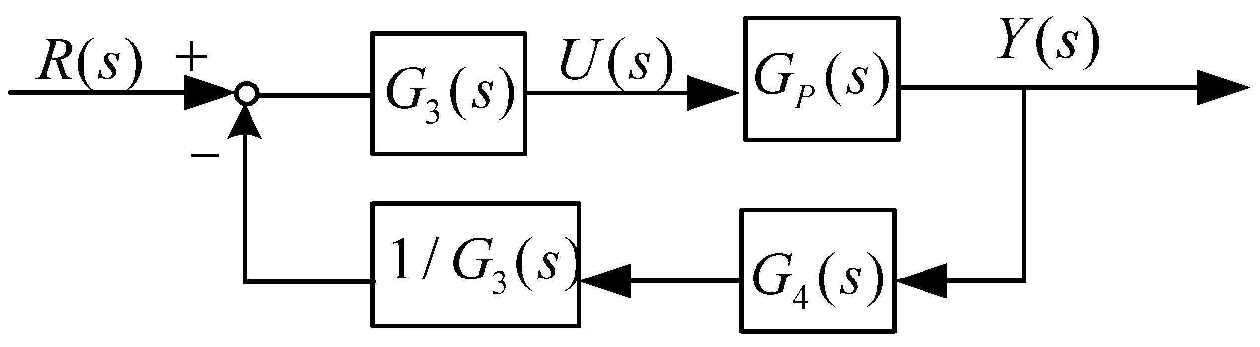
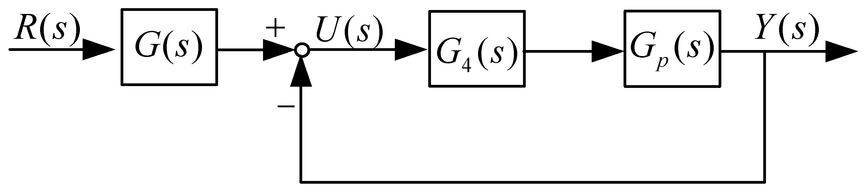
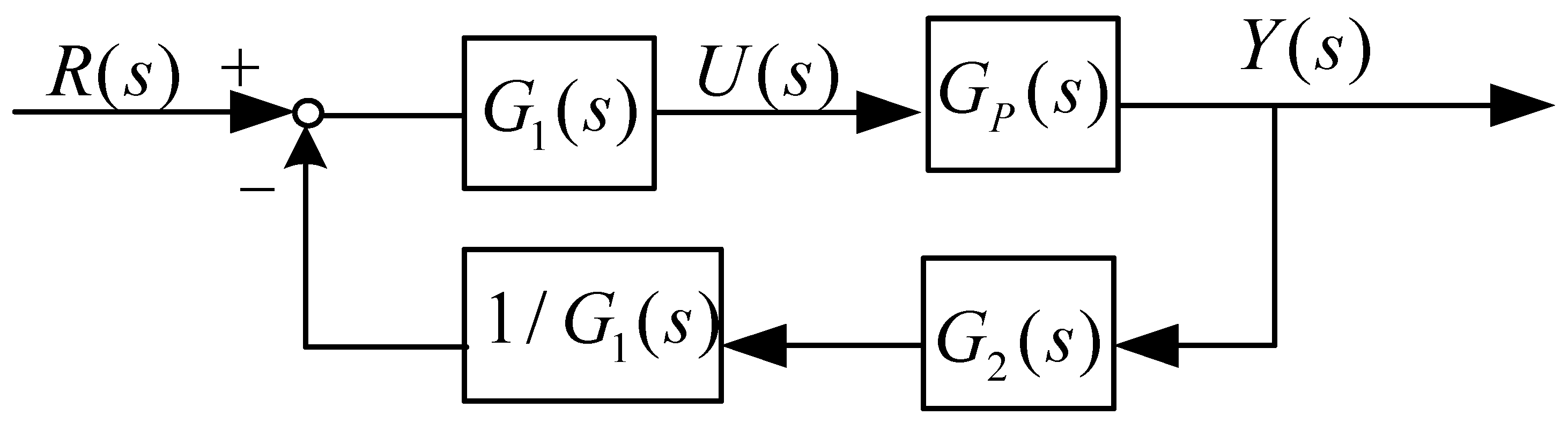
4.1. IMP-ESO-ADRC Design

To facilitate discussion, this study considers implementing the IMP-ESO proposed in Section 3 on a second-order system, and integrating it within an ADRC controller. Accordingly, the corresponding state feedback control law utilized herein may be expressed as follows, as cited from reference [26]:

Applying the Laplace transform to Equation (4), we obtain:

$$\{\begin{array}{l}s{\widehat{X}}_1(s)={\widehat{X}}_2(s)+{\beta }_1(X_1(s)-{\widehat{X}}_1(s))\\ s{\widehat{X}}_2(s)={\widehat{X}}_3(s)+{\beta }_2(X_1(s)-{\widehat{X}}_1(s))+\overline{b}U(s)\\ s{\widehat{X}}_3(s)=G_z(s)(X_1(s)-{\widehat{X}}_1(s))\end{array}$$

(21)

Applying iteration to Equation (21), we obtain:

$$\{\begin{array}{l}{\widehat{X}}_1(s)={\beta }_1{s}^{-1}\left(X_1(s)-{\widehat{X}}_1(s)\right)+{\beta }_2{s}^{-2}\left(X_1(s)-{\widehat{X}}_1(s)\right)+\frac{1}{s^2}\overline{b}U(s)\\ {\widehat{X}}_2(s)={\beta }_2{s}^{-1}\left(X_1(s)-{\widehat{X}}_1(s)\right)+{\beta }_3{s}^{-2}\left(X_1(s)-{\widehat{X}}_1(s)\right)+\frac{1}{s}\overline{b}U(s)\\ {\widehat{X}}_3(s)=G_z(s)s^{-1}\left(X_1(s)-{\widehat{X}}_1(s)\right)\end{array}$$

(22)

By applying the Laplace transform to the expanded state Equation (2) of the system, we can derive its transfer function as follows:

$$\{\begin{array}{l}s{X}_1(s)=X_2(s)\\ s{X}_2(s)=X_3(s)+\overline{b}U(s)\end{array}$$

(23)

From the state feedback control law, we can obtain its transfer function as follows:

$$\begin{array}{l}U(s)=\frac{k_{2}R(s)}{\overline{b}}-\frac{X_3(s)+k_2{\widehat{X}}_1(s)+k_1{\widehat{X}}_2(s)}{\overline{b}}\\ \hspace{1em}\hspace{1em}=\frac{k_{2}R(s)-(X_3(s)+k_2{\widehat{X}}_1(s)+k_1{\widehat{X}}_2(s))}{\overline{b}}\end{array}$$

(24)

From the first equation in Equation (22), we can derive the following:

$${\widehat{X}}_1(s)=\frac{({\beta }_1{s}^2+{\beta }_{2}s+G_z)X_1(s)+\overline{b}sU(s)}{s^3+{\beta }_1{s}^2+{\beta }_{2}s+G_z(s)}$$

(25)

By substituting Equations (22) and (25) into Equation (24), we can obtain the following expression:

$$\begin{array}{l}U(s)=\frac{k_{1}R(s)-(X_3(s)+k_2{\widehat{X}}_1(s)+k_1{\widehat{X}}_2(s))}{\overline{b}}\\ \hspace{1em}\hspace{1em}=\frac{k_1}{\overline{b}}\frac{c_2(s)R(s)}{b_2(s)}-\frac{1}{\overline{b}}\frac{a_2(s)}{b_2(s)}{X}_1(s)\end{array}$$

(26)

where:

$$\begin{array}{l}{a}_2(s)=k_2(G_z(s)+{\beta }_{2}s+{\beta }_1{s}^2)+k_1(s{G}_z(s)+{\beta }_2{s}^2)+s^3{G}_z(s)\\ b_2(s)=s^3+{\beta }_{2}s+{\beta }_1{s}^2+G_z(s)+k_{2}s+k_1(s^2+{\beta }_{1}s)-s{G}_z(s)\\ c_2(s)=s^3+{\beta }_{2}s+{\beta }_1{s}^2+G_z(s)\end{array}$$

Because $X_1(s)=Y(s)$, we can finally obtain:

$$U(s)=\frac{1}{\overline{b}}\frac{C_2(s)R(s)-A_2(s)Y(s)}{B_2(s)}$$

(27)

where:

$$\begin{array}{l}{A}_2(s)=k_2(G_z(s)+{\beta }_{2}s+{\beta }_1{s}^2)+k_1(s{G}_z(s)+{\beta }_2{s}^2)+s^3{G}_z(s)\\ B_2(s)=s^3+{\beta }_{2}s+{\beta }_1{s}^2+G_z(s)+k_{2}s+k_1(s^2+{\beta }_{1}s)-s{G}_z(s)\\ C_2(s)=k_1(s^3+{\beta }_{2}s+{\beta }_1{s}^2+G_z(s))\end{array}$$

Therefore, from Equation (27), we can derive Equation (28) as follows:

$$U(s)=G_3(s)R(s)-G_4(s)Y(s)$$

(28)

Based on the derived equations, we can illustrate the closed-loop control of the ADRC system using IMP-ESO as shown in Figure 2:

Based on the equivalence transformation from Figure 2, we can derive the closed-loop control principle block diagram of ADRC based on IMP-ESO, as shown in Figure 3:

From Figure 3, we can determine the equivalent unit negative feedback open-loop transfer function of the ADRC closed-loop control system based on IMP-ESO as follows:

$$G_{o2}(s)=G_p(s)\cdot G_4(s)$$

(29)

By applying further shift transformation to Figure 2, we can obtain the following closed-loop control block diagram of IMP-ESO-ADRC:

In the depicted diagram $G(s)=\frac{G_3(s)}{G_4(s)}=\frac{C_2(s)}{A_2(s)}$, it can be observed that a lead-lag element is employed, along with input shaping to enhance the stability of the closed-loop control system. In the design scheme presented in Figure 4, for different disturbance characteristics, a new transfer function can be constructed to achieve error-free tracking and observation of disturbances. This enables precise control of the ADRC control system.

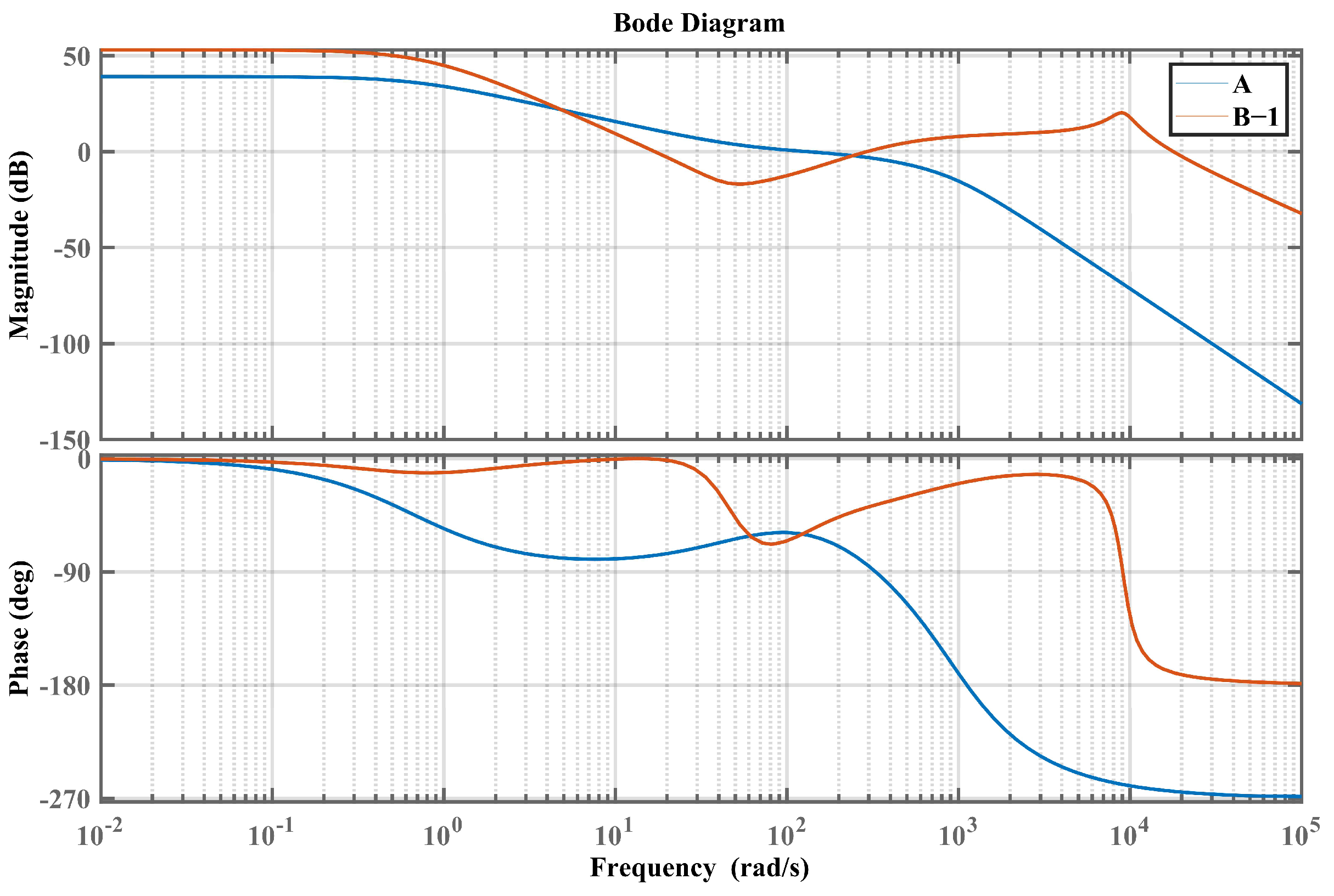
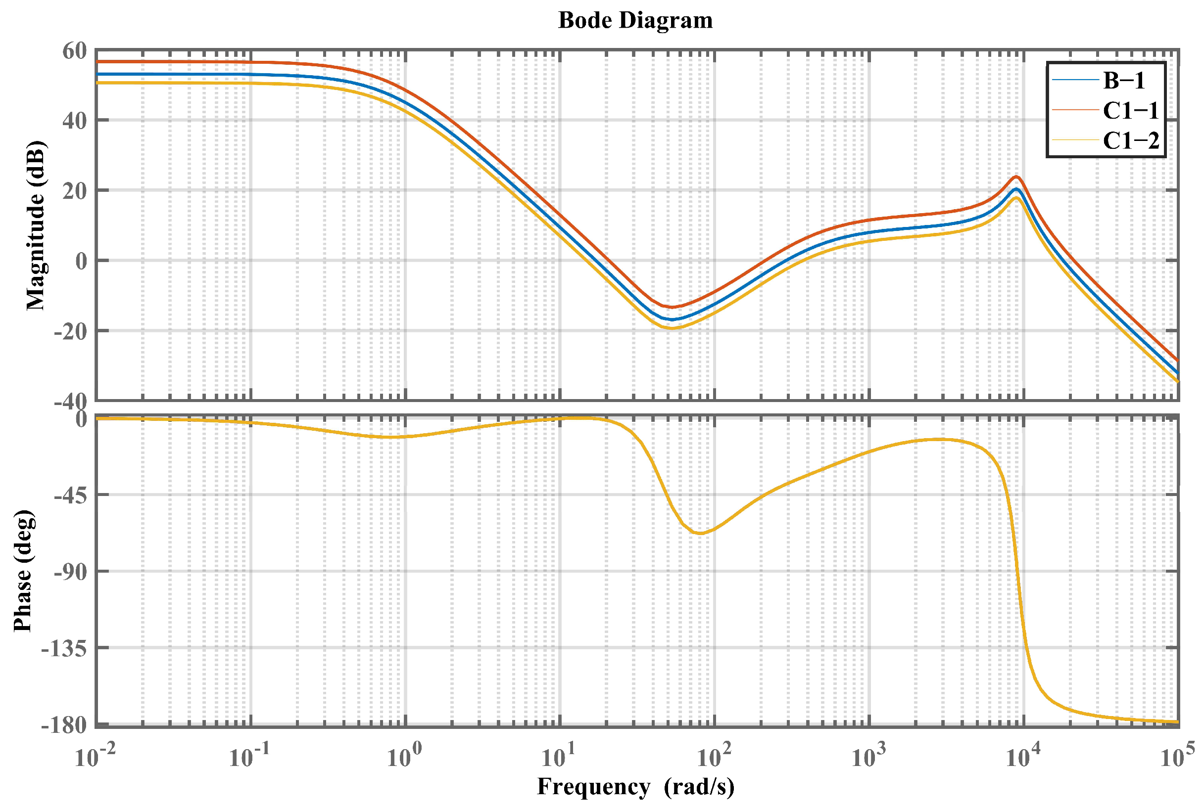
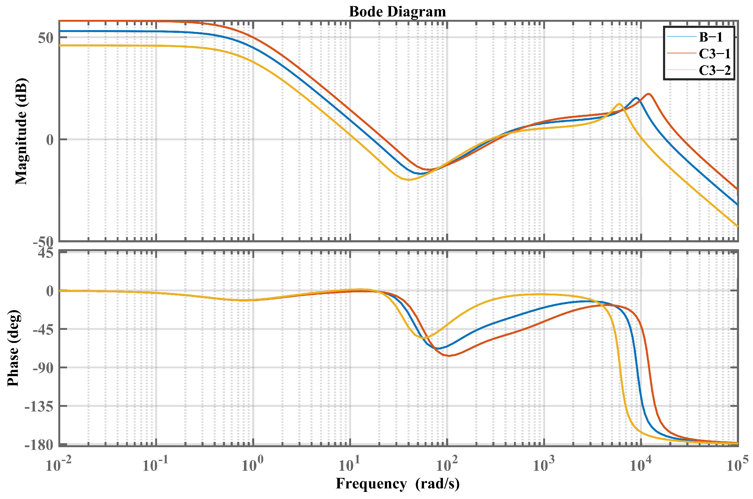
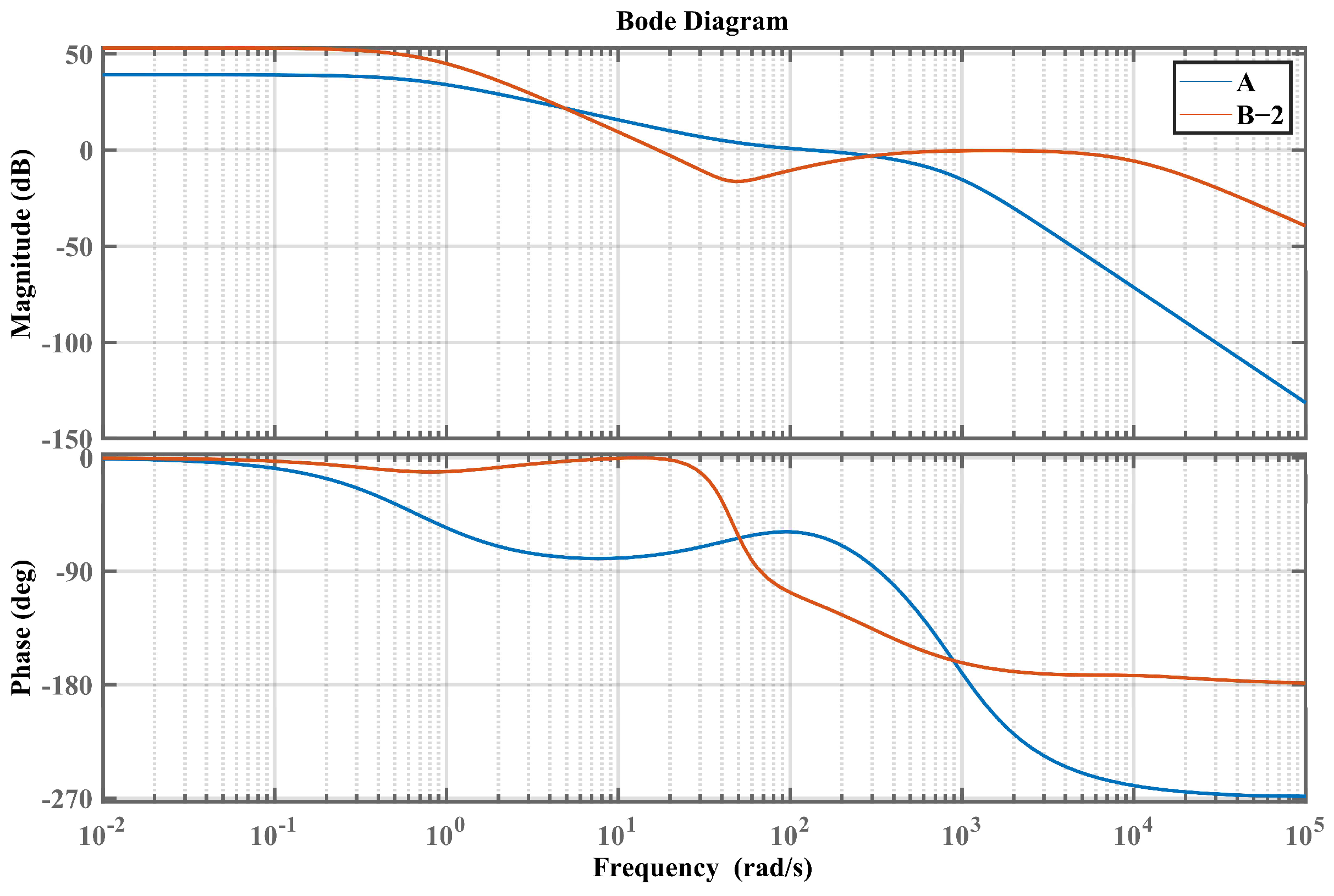
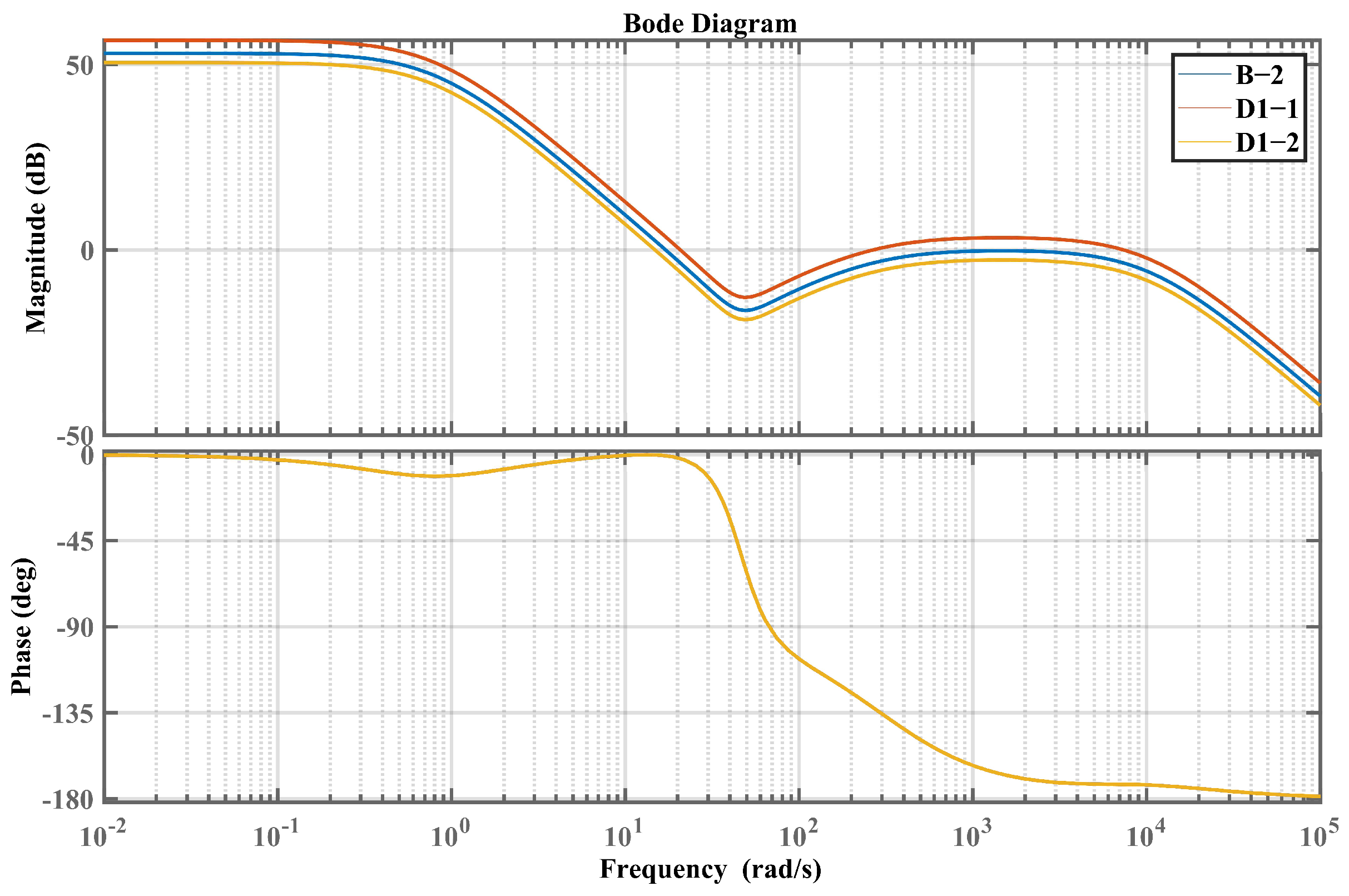
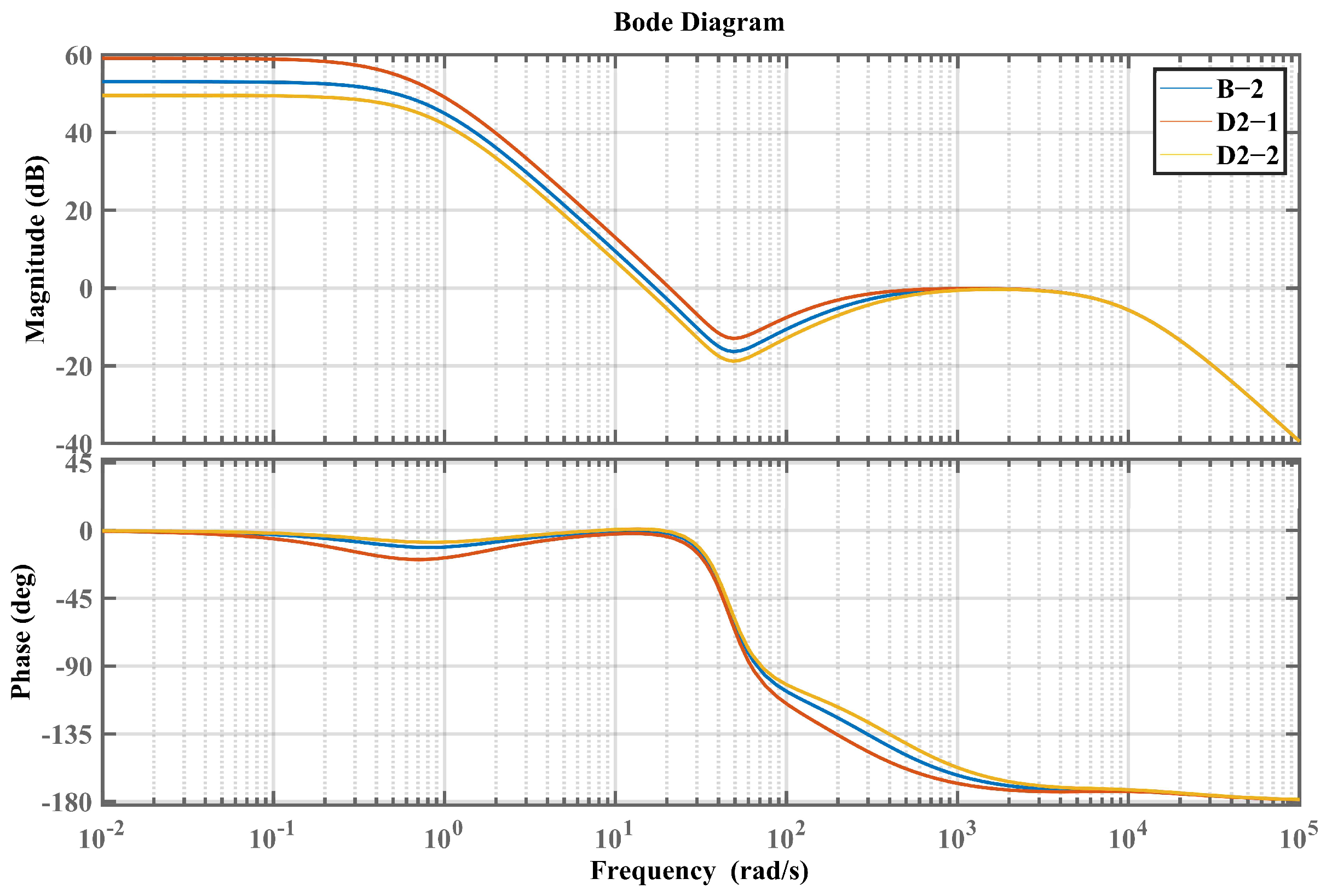
4.2. Frequency Domain Analysis

Frequency analysis and simulation comparison play an integral role in evaluating the performance of the ESO-ADRC system. In this section, we will conduct a comprehensive analysis of stability indicators, such as phase margin, gain margin, and crossover frequency, based on the equivalent unit negative feedback open-loop transfer function derived from IMP-ESO-ADRC. By comparing the results obtained from simulations, we can assess the effectiveness of the proposed control scheme and its ability to handle various disturbance characteristics.

The design process for the traditional ESO-ADRC follows the same principles as discussed in Section 4.1. By applying the traditional ESO and integrating it into the ADRC controller, we can obtain the corresponding state feedback control law.

$$U(s)=\frac{1}{\overline{b}}\frac{C(s)R(s)-A_1(s)Y(s)}{B_1(s)}$$

(30)

where:

$$\begin{array}{l}{A}_1(s)=s^{2}A={\displaystyle {\sum }_{i=0}^2({\displaystyle {\sum }_{j=0}^{2-i}{k}_{i+j}{\beta }_{3-j}})s^{1-i}}\hspace{1em}\\ B_1(s)={\displaystyle {\sum }_{i=0}^2({\displaystyle {\sum }_{j=0}^i{k}_j{\beta }_{i-j}})s^{n-i}}\\ C(s)=k_{2}C=k_2{\displaystyle {\sum }_{i=0}^3{\beta }_i{s}^{2-i}}\end{array}$$

Let: $G_1(s)=\frac{C(s)}{\overline{b}{B}_1(s)},G_2(s)=\frac{A_1(s)}{\overline{b}{B}_1(s)}$.

From Equation (26), we can deduce:

$$U(s)=G_1(s)R(s)-G_2(s)Y(s)$$

(31)

Based on this, we can derive the control block diagram of the system as shown in Figure 5:

Indeed, it is evident that from Figure 5, we can derive the block diagram illustrating the closed-loop control principle of the ADRC system, as depicted in Figure 6:

From Figure 6, we can obtain the equivalent unit negative feedback open-loop transfer function of the ADRC closed-loop control system for System (1) as follows:

$$G_{o1}(s)=G_p(s)\cdot G_2(s)$$

(32)

In the traditional ESO-ADRC, the selection of observer parameters and state feedback control parameters follows the principle of pole-zero cancellation [11]. Therefore, we have:

$$\begin{array}{l}{\beta }_1=3{\omega }_o,{\beta }_2=3{\omega }_o^2,{\beta }_3={\omega }_o^3\\ k_1=2{\omega }_c,k_2={\omega }_c^2\end{array}$$

Therefore, it can be inferred that:

$$A_1(s)=\frac{({\omega }_o^3+6{\omega }_c{\omega }_o^2+3{\omega }_c^2{\omega }_o){\omega }_c^2{\omega }_o^3{s}^2}{{\omega }_c^2{\omega }_o^{3}s}+\frac{(2{\omega }_c{\omega }_o^3+3{\omega }_c^2{\omega }_o^2){\omega }_c^2{\omega }_o^{3}s+1}{{\omega }_c^2{\omega }_o^{3}s}$$

(33)

$$B_1(s)=s^2+(3{\omega }_o+2{\omega }_c)s+(3{\omega }_o^2+6{\omega }_c{\omega }_o+{\omega }_c^2)$$

(34)

The transfer function of system is given by:

$$G_p=\frac{b}{s^2+a_{1}s+a_2}$$

(35)

Finally, we can determine the equivalent unit negative feedback open-loop transfer function of the traditional ESO-ADRC closed-loop system for System (35) as follows:

$$G_{o1}(s)=G_p(s)\cdot \frac{A_1(s)}{\overline{b}{B}_1(s)}$$

(36)

(1) Harmonic Disturbances

We can derive the transfer function of the IMP-ESO-ADRC system, as well as its $A_3(s)$ and $B_3(s)$, based on Equation (27):

$$A_3(s)={{\omega }_c}^2[G_{z1}(s)+(9{{\omega }_0}^2-{{\omega }_n}^2)s+5{\omega }_0{s}^2]+2{\omega }_c[s{G}_{z1}(s)+(9{{\omega }_0}^2-{{\omega }_n}^2)s^2]+s^3{G}_{z1}(s)$$

(37)

$$B_3(s)=s^3+(9{{\omega }_0}^2-{{\omega }_n}^2)s+5{\omega }_0{s}^2+G_{z1}(s)+{{\omega }_c}^{2}s+2{\omega }_c(s^2+5{\omega }_{0}s)-s{G}_{z1}(s)$$

(38)

where:

$$G_{z1}(s)=\frac{(9{{\omega }_0}^3-5{\omega }_0{{\omega }_n}^2)s^2+(5{{\omega }_0}^4-9{{\omega }_0}^2{{\omega }_n}^2+{{\omega }_n}^4)s+{{\omega }_0}^5}{s^2+{{\omega }_n}^2}$$

Finally, we can determine the equivalent unit negative feedback open-loop transfer function of the second-order system using IMP-ESO-ADRC as follows:

$$G_{o2}(s)=G_p(s)\cdot \frac{A_3(s)}{\overline{b}{B}_3(s)}$$

(39)

In this study, the harmonic signal used has an amplitude of two and a frequency of ω, denoted as f.

Table 1. Second-order system and control parameters.

System	${\mathit{a}}_1$	${\mathit{a}}_2$	b	$\overline{\mathit{b}}$	${\mathit{\omega }}_{\mathit{o}}$	${\mathit{\omega }}_{\mathit{c}}$
A	300	200	400	400	300	300
B-1	300	200	400	400	300	300
C1-1	300	200	600	400	300	300
C1-2	300	200	300	400	300	300
C2-1	200	100	400	400	300	300
C2-2	400	300	400	400	300	300
C3-1	300	200	400	400	400	400
C3-2	300	200	400	400	200	200

presents the frequency characteristics of the IMP-ESO-ADRC closed-loop control system based on different system and control parameters. It compares stability indicators such as gain margin, phase margin, and crossover frequency for varying system and control parameter configurations.

Using MATLAB programming simulations, Figure 7, Figure 8, Figure 9 and Figure 10 depict the Bode plots that compare the equivalent unit negative feedback open-loop systems of A (note: A represents the traditional ESO-ADRC), C1-1, C1-2, C2-1, C2-2, and B-1 (note: C1-1, C1-2, C2-1, C2-2, and B-1 system represents the IMP-ESO-ADRC under the influence of harmonic disturbances) closed-loop control systems.

Table 2. Stability indicators of the closed-loop control systems based on Table 1.

System	Cutoff Frequency (rad/s)	Crossover Frequency (rad/s)	Gain Margin (dB)	Phase Margin (Degrees)	Delay Margin (s)	Stability
A	133	297	17.3	119	0.0156	Stable
B-1	17	20.1	-	180	0.184	Stable
C1-1	20.7	24.3	-	179	0.151	Stable
C1-2	14.8	17.5	-	180	0.212	Stable
C2-1	20.6	24.2	-	176	0.149	Stable
C2-2	14.8	17.6	-	179	0.213	Stable
C3-1	22.7	26.8	-	178	0.137	Stable
C3-2	11.3	13.4	-	179	0.28	Stable

provides a comparison of stability indicators for the following four scenarios:

• Comparison between A and B-1;
• Comparison between B-1 and C1-1, C1-2;
• Comparison between B-1 and C2-1, C2-2;
• Comparison between B-1 and C3-1, C3-2.

Based on the parameters of system A, the traditional ESO-ADRC closed-loop control system and the closed-loop system B-1 have identical parameters. From the analysis of Figure 7 and Table 2, it can be concluded that IMP-ESO-ADRC has a larger bandwidth compared to traditional ESO-ADRC. Therefore, it exhibits faster response speed, stronger disturbance rejection capability, and greater robustness against rapidly changing disturbances. The phase of IMP-ESO-ADRC does not exceed −180°, thus there is no corresponding gain margin.

For the IMP-ESO-ADRC closed-loop control system based on parameters C1-1 and C1-2, only the system gain $\overline{b}$ of the reference closed-loop system B-1 is modified. From the analysis of Figure 8 and Table 2, it can be observed that as the ratio of the system gain to the nominal gain of IMP-ESO-ADRC increases, the phase margin, crossover frequency, and cutoff frequency also increase, while the delay margin remains almost unchanged.

Similarly, for the IMP-ESO-ADRC closed-loop control system based on parameters C2-1 and C2-2, adjustments are made to the controlled system coefficients $a_1$ and $a_2$ of the reference closed-loop system B-1. From the analysis of Figure 9 and Table 2, it can be observed that as the values of the controlled system coefficients $a_1$ and $a_2$ increase, the phase margin, crossover frequency, and cutoff frequency increase, while the delay margin remains almost unchanged.

Furthermore, for the IMP-ESO-ADRC closed-loop control system based on parameters C3-1 and C3-2, modifications are made to the observation bandwidth  ${\omega }_o$ and control bandwidth ${\omega }_c$ of IMP-ESO-ADRC relative to the reference system B-1. From the analysis of Figure 10 and Table 2, it can be observed that as the observation bandwidth ${\omega }_o$ and control bandwidth ${\omega }_c$ of IMP-ESO-ADRC increase, the crossover frequency, cutoff frequency, and phase margin increase, while the delay margin remains almost unchanged.

From the simulation results of Figure 8, Figure 9 and Figure 10 and Table 2, it can be concluded that although the variations in the controlled system coefficients $a_1,a_2$ and IMP-ESO-ADRC parameters ${\omega }_o,{\omega }_c,\overline{b}$ have a wide range, they do not affect the stability of the IMP-ESO-ADRC closed-loop control system under harmonic disturbances. This fully demonstrates the strong robustness of control systems based on IMP-ESO-ADRC.

(2) Ramp Disturbances

Similarly, by applying Equation (27), we can also derive the expressions for $A_4(s)$ and $B_4(s)$ of the IMP-ESO-ADRC.

$$A_4(s)={{\omega }_c}^2[G_{z2}(s)+(9{{\omega }_0}^2-{{\omega }_n}^2)s+5{\omega }_0{s}^2]+2{\omega }_c[s{G}_{z2}(s)+(9{{\omega }_0}^2-{{\omega }_n}^2)s^2]+s^3{G}_{z2}(s)$$

(40)

$$B_4(s)=s^3+(9{{\omega }_0}^2-{{\omega }_n}^2)s+5{\omega }_0{s}^2+G_{z2}(s)+{{\omega }_c}^{2}s+2{\omega }_c(s^2+5{\omega }_{0}s)-s{G}_{z2}(s)$$

(41)

where:

$$G_{z2}(s)=\frac{4{{\omega }_0}^{3}s+{{\omega }_0}^4}{s}$$

Finally, we can determine the equivalent unit negative feedback open-loop transfer function of the second-order system using IMP-ESO-ADRC as follows:

$$G_{o2}(s)=G_p(s)\cdot \frac{A_4(s)}{\overline{b}{B}_4(s)}$$

(42)

Based on the various system parameters and control parameters provided in

Table 3. Second-order system and control parameters.

System	${\mathit{a}}_1$	${\mathit{a}}_2$	b	$\overline{\mathit{b}}$	${\mathit{\omega }}_{\mathit{o}}$	${\mathit{\omega }}_{\mathit{c}}$
A	300	200	400	400	300	300
B-2	300	200	400	400	300	300
D1-1	300	200	600	400	300	300
D1-2	300	200	300	400	300	300
D2-1	200	100	400	400	300	300
D2-2	400	300	400	400	300	300
D3-1	300	200	400	400	400	400
D3-2	300	200	400	400	200	200

, we conducted a comparative study on the stability indicators, including gain margin, phase margin, and crossover frequency, of the IMP-ESO-ADRC closed-loop system. By employing the IMP-ESO-ADRC controller, we analyzed the effects of different system and control parameters on the stability of the closed-loop system.

To conduct the study, we utilized MATLAB programming for simulation purposes. Specifically, we plotted Figure 11, Figure 12, Figure 13 and Figure 14, which represent the Bode plots of the equivalent unity feedback open-loop systems for A, D1-1, D1-2, D2-1, D2-2, and B-2 (note: D1-1, D1-2, D2-1, D2-2, and B-2 system represents the IMP-ESO-ADRC under the influence of harmonic disturbances) closed-loop control systems.

Furthermore,

Table 4. Stability indicators of the closed-loop control systems based on Table 3.

System	Cutoff Frequency (rad/s)	Crossover Frequency (rad/s)	Gain Margin (dB)	Phase Margin (Degrees)	Delay Margin (s)	Stability
A	133	296	17.3	119	0.0156	Stable
B	17.1	20	-	179	0.183	Stable
D1-1	20.8	24.5	-	178	0.15	Stable
D1-2	14.8	17.6	-	180	0.211	Stable
D2-1	20.7	24.4	-	176	0.148	Stable
D2-2	14.8	17.6	-	179	0.213	Stable
D3-1	22.8	26.7	-	177	0.136	Stable
D3-2	11.4	13.5	-	179	0.278	Stable

provides a comprehensive comparison of the stability indicators for the following four scenarios:

• Comparison between A and B-2;
• Comparison between B-2 and D1-1, D1-2;
• Comparison between B-2 and D2-1, D2-2;
• Comparison between B-2 and D3-1, D3-2.

This comparative analysis allows us to evaluate the impact of different system and control parameters on the stability performance of the closed-loop control systems.

Please note that the simulation results and the comparative analysis presented in Figure 11, Figure 12, Figure 13 and Figure 14, and Table 4 provide valuable insights into the performance and stability characteristics of the IMP-ESO-ADRC closed-loop control system.

The results obtained from the analysis of Figure 11 and Table 4 reveal that IMP-ESO-ADRC exhibits a larger bandwidth compared to traditional ESO-ADRC, indicating faster response speed and increased robustness in the face of fast-changing disturbances. It is noteworthy that the phase of IMP-ESO-ADRC does not exceed −180°, implying the absence of corresponding gain margin.

Furthermore, by considering the IMP-ESO-ADRC closed-loop control system based on parameters D1-1 and D1-2, which only modify the system gain $b$ of the reference closed-loop system B-1, analysis from Figure 12 and Table 4 demonstrates that a higher ratio between the system gain and the nominal gain of IMP-ESO-ADRC leads to a larger phase margin, higher crossover frequency, and cutoff frequency, with negligible changes in delay margin.

Similarly, for the IMP-ESO-ADRC closed-loop control system based on parameters D2-1 and D2-2, which adjust the controlled system coefficients $a_1$ and $a_2$ of the reference closed-loop system B-1, analysis from Figure 13 and Table 4 indicates that larger values of the controlled system coefficients $a_1$ and $a_2$ result in a larger phase margin, higher crossover frequency, and cutoff frequency, while the delay margin remains almost unchanged.

Additionally, the IMP-ESO-ADRC closed-loop control system based on parameters D3-1 and D3-2 modifies the observation bandwidth and control bandwidth of IMP-ESO-ADRC relative to the reference system B-1. Analysis from Figure 14 and Table 4 shows that increasing the observation bandwidth and control bandwidth of IMP-ESO-ADRC leads to a higher crossover frequency, cutoff frequency, and larger phase margin, with minimal changes in delay margin.

The simulation results from Figure 12, Figure 13 and Figure 14 and Table 4 clearly demonstrate that variations in the controlled system coefficients and IMP-ESO-ADRC parameters do not affect the stability of the IMP-ESO-ADRC closed-loop control system under ramp disturbance. This provides strong evidence for the robustness of the control system based on IMP-ESO-ADRC.

5. Simulation Test Results and Analysis

To validate the performance of the IMP-ESO-ADRC control system, simulation testing was conducted. The purpose of these tests was to assess the effectiveness and robustness of the IMP-ESO-ADRC in various scenarios.

The simulation environment was set up using MATLAB, and the IMP-ESO-ADRC controller was implemented according to the specified parameters and control strategies. The system response, stability, and disturbance rejection capabilities were evaluated through a series of simulated experiments.

During the simulation testing, different input signals and disturbance profiles were applied to the system to evaluate its dynamic response and robustness. The performance of the IMP-ESO-ADRC control system was then analyzed based on various metrics such as tracking accuracy and steady-state error.

Additionally, comparisons were made between the IMP-ESO-ADRC control system and ESO-ADRC control system strategies to assess its advantages and limitations. The simulation results were carefully analyzed and interpreted to gain insights into the behavior and performance of the IMP-ESO-ADRC under different operating conditions.

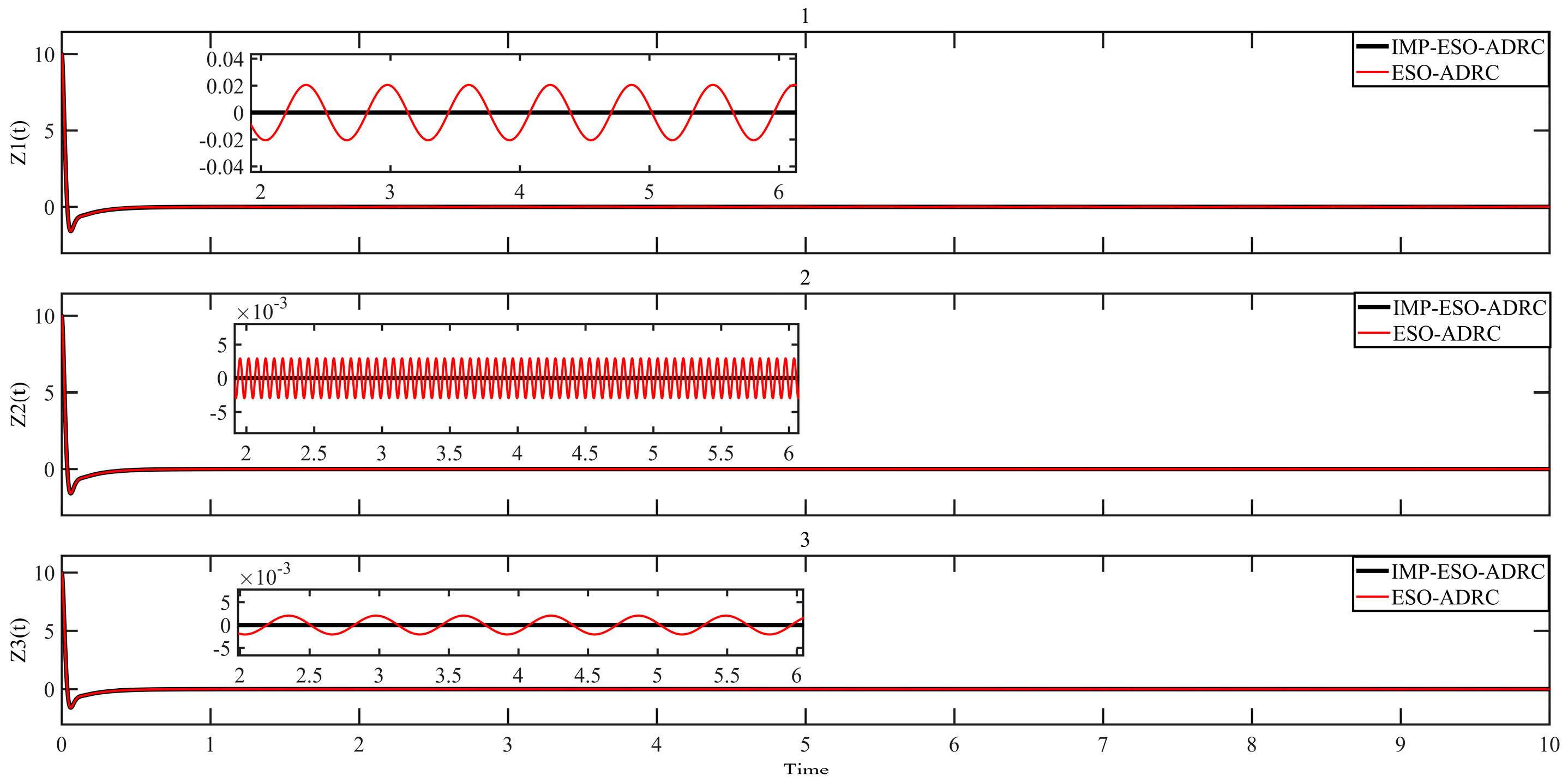
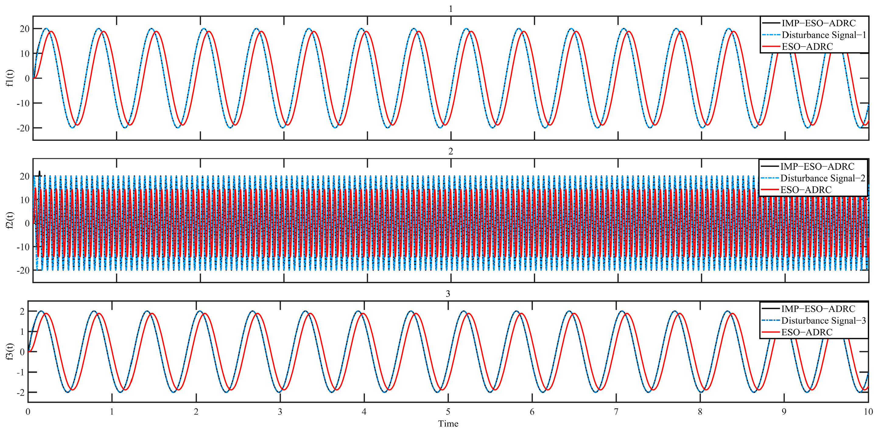
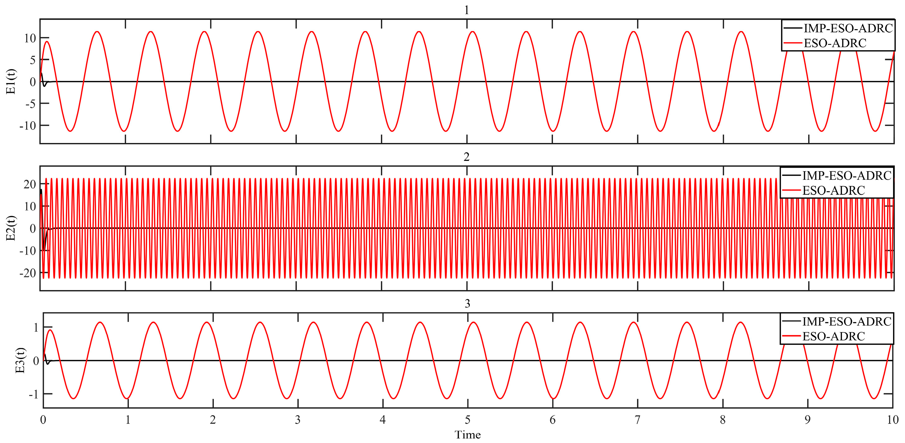
5.1. Simulation with Harmonic Disturbance

During the simulation, a step signal with a magnitude of 10 was applied as the input signal to the system. Three different sets of disturbance signals, denoted as $f_1=20\sin (10t)$, $f_2=20\sin (100t)$, and $f_3=2\sin (10t)$, were added to assess the performance of both traditional ESO-ADRC and IMP-ESO-ADRC control strategies.

Figure 15 and Figure 16 provide a comparison of the control response speed and control accuracy ($Z(t)=y(t)-r(t)$) between traditional ESO-ADRC and IMP-ESO-ADRC. On the other hand, Figure 17 and Figure 18 present a comparison of disturbance tracking speed and disturbance tracking error ($E(t)=f(t)\stackrel{⌢}{-}{\widehat{x}}_3(t)$) between traditional ESO-ADRC and IMP-ESO-ADRC.

From Figure 18, it can be observed that IMP-ESO-ADRC exhibits a significantly lower disturbance tracking error, with a maximum absolute mean error value of 0.0003. Furthermore, the performance of IMP-ESO-ADRC remains unaffected by variations in external disturbance harmonic frequency and amplitude. In contrast, traditional ESO-ADRC shows a maximum absolute mean error value of 21.2471 and a minimum of 1.1376 when external disturbance harmonic frequency and amplitude change.

Figure 16 provides additional insights, showing that the maximum absolute mean control error for IMP-ESO-ADRC is 0.000004, whereas for traditional ESO-ADRC it ranges from 0.0032 to 0.0217. Thus, based on the simulation results, it is evident that IMP-ESO-ADRC demonstrates superior error tracking capability and enhanced disturbance rejection ability.

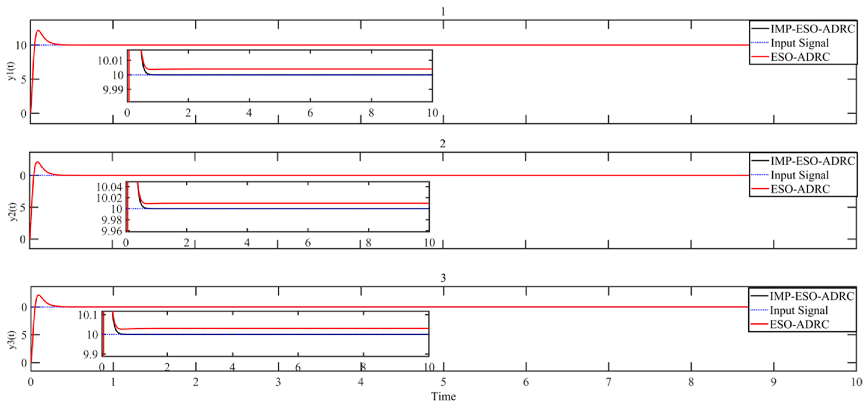
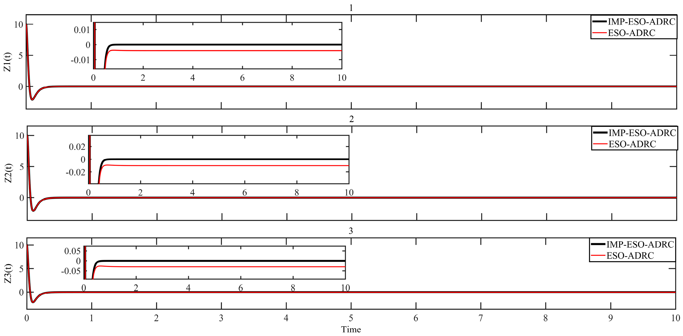
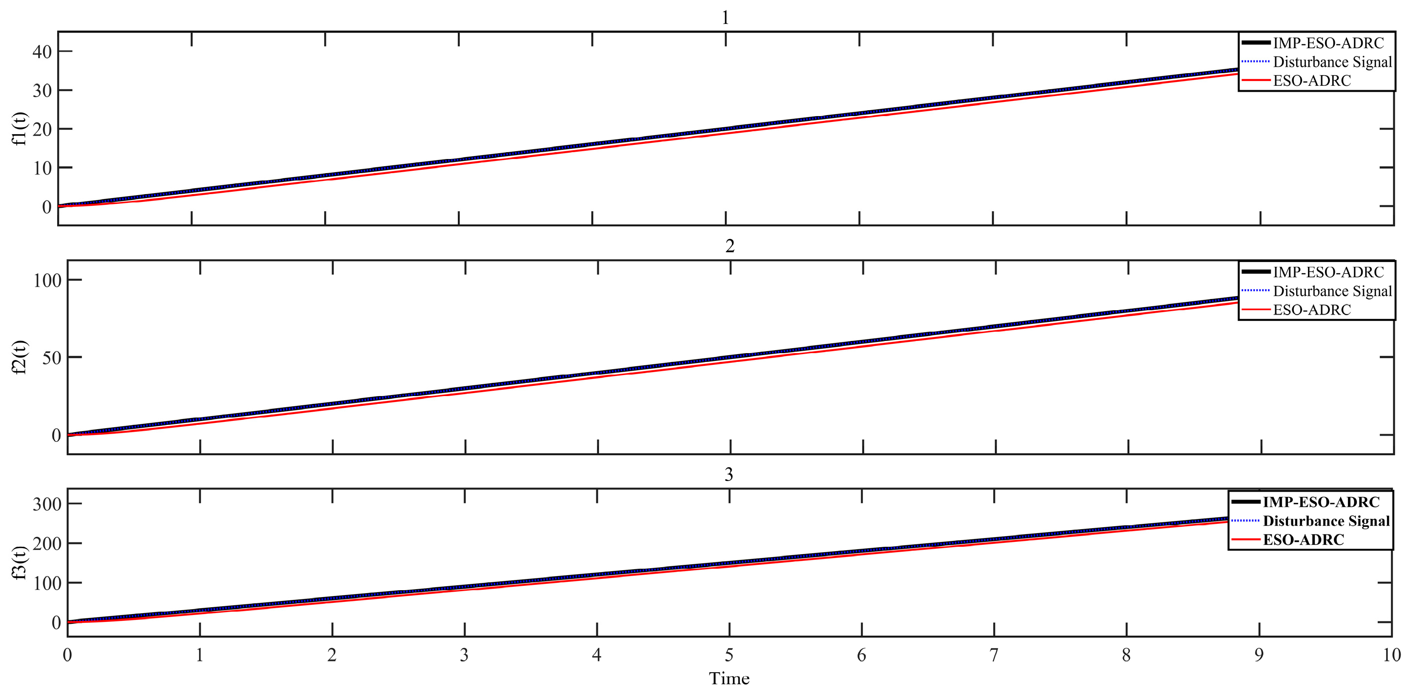
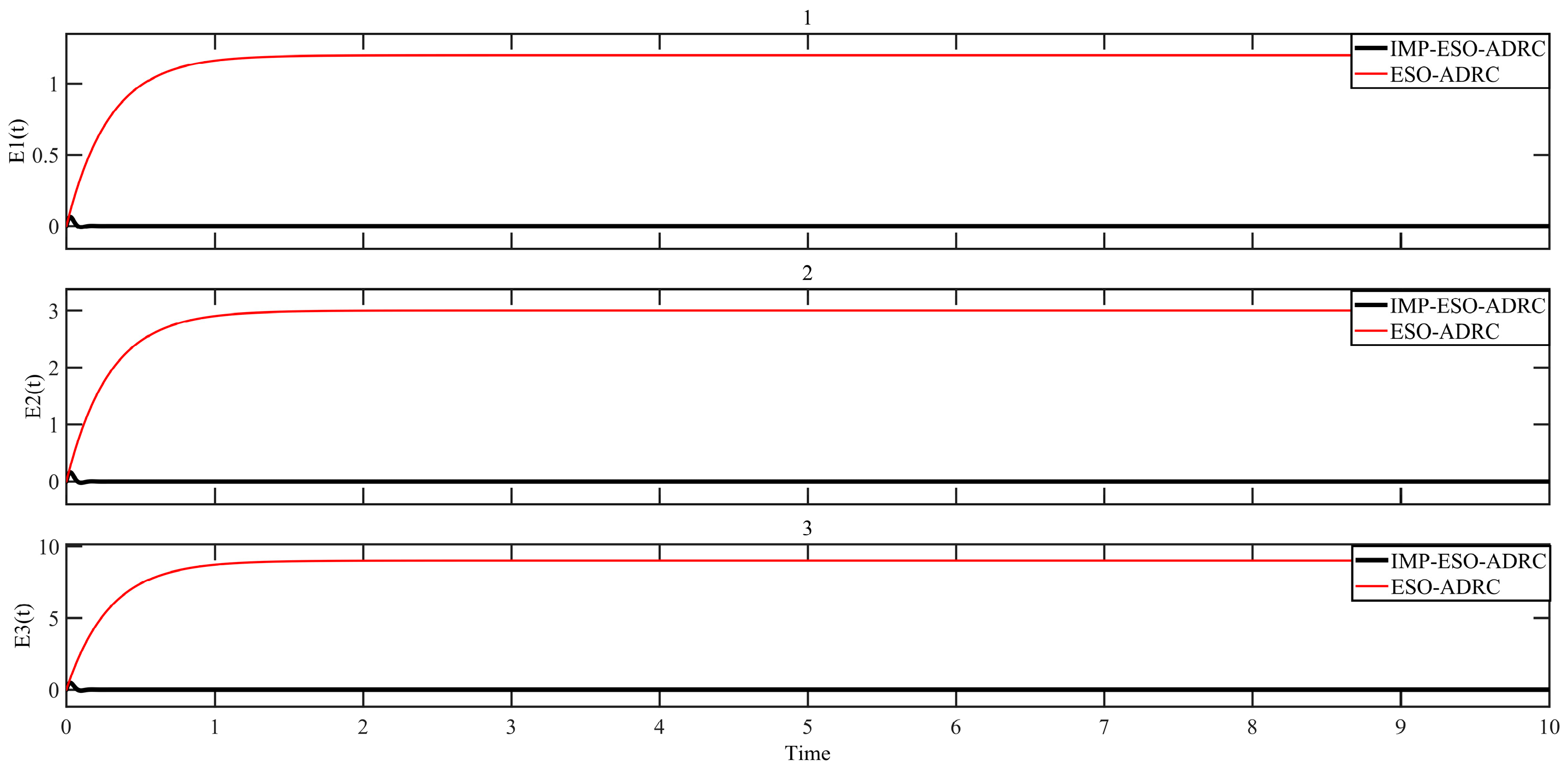
5.2. Simulation with Ramp Disturbance

In the simulation, a step signal with a magnitude of 10 was applied as the input signal to the system. Three different sets of ramp disturbance signals with ramp of 4, 10, and 30 were added. Figure 19 and Figure 20 provide a comparison of the control response speed and control accuracy between traditional ESO-ADRC and IMP-ESO-ADRC. On the other hand, Figure 21 and Figure 22 present a comparison of disturbance tracking speed and disturbance tracking error between traditional ESO-ADRC and IMP-ESO-ADRC.

From Figure 22, it can be observed that IMP-ESO-ADRC exhibits a significantly lower disturbance tracking error, with a maximum absolute mean error value of 0.0001. Furthermore, the performance of IMP-ESO-ADRC remains unaffected by variations in the slope of the external ramp disturbance. In contrast, traditional ESO-ADRC shows a maximum absolute mean error value of 8.0732 and a minimum of 1.1268 when the slope of the external ramp disturbance changes.

Figure 20 provides additional insights, showing that the maximum absolute mean control error for IMP-ESO-ADRC is 0.000002, whereas for traditional ESO-ADRC it ranges from 0.0051 to 0.0284. Thus, based on the simulation results, it is evident that IMP-ESO-ADRC demonstrates a superior error tracking capability and enhanced disturbance rejection ability.

From the simulation results, it is apparent that the proposed IMP-ESO-ADRC not only tracks non-constant disturbances effectively but also exhibits excellent tracking performance for high-frequency harmonic disturbances. Compared to traditional ESO-ADRC, IMP-ESO-ADRC significantly improves disturbance tracking performance, particularly in the presence of large-amplitude harmonic disturbances. Therefore, IMP-ESO-ADRC exhibits superior disturbance rejection ability when facing disturbances.

Additionally, in the stable stage, IMP-ESO-ADRC exhibits higher input tracking accuracy compared to traditional ADRC and can rapidly track disturbance signals. Thus, compared to traditional ADRC, the proposed IMP-ESO-ADRC offers advantages such as higher tracking accuracy and stronger disturbance rejection capability. It demonstrates robustness in the presence of non-constant disturbances and is particularly suitable for systems with high-frequency disturbances. It effectively suppresses system vibrations and enhances system precision and stability.

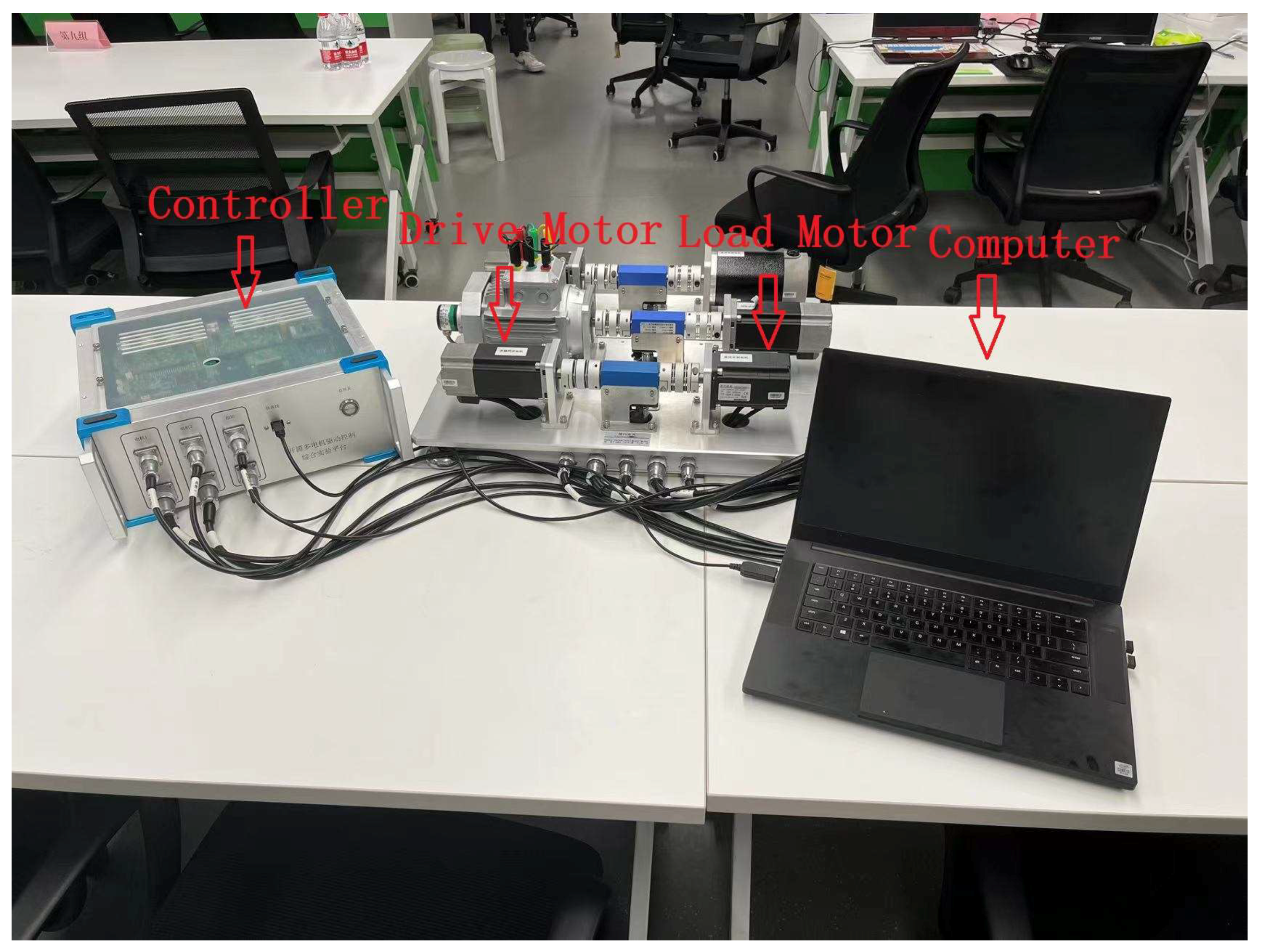
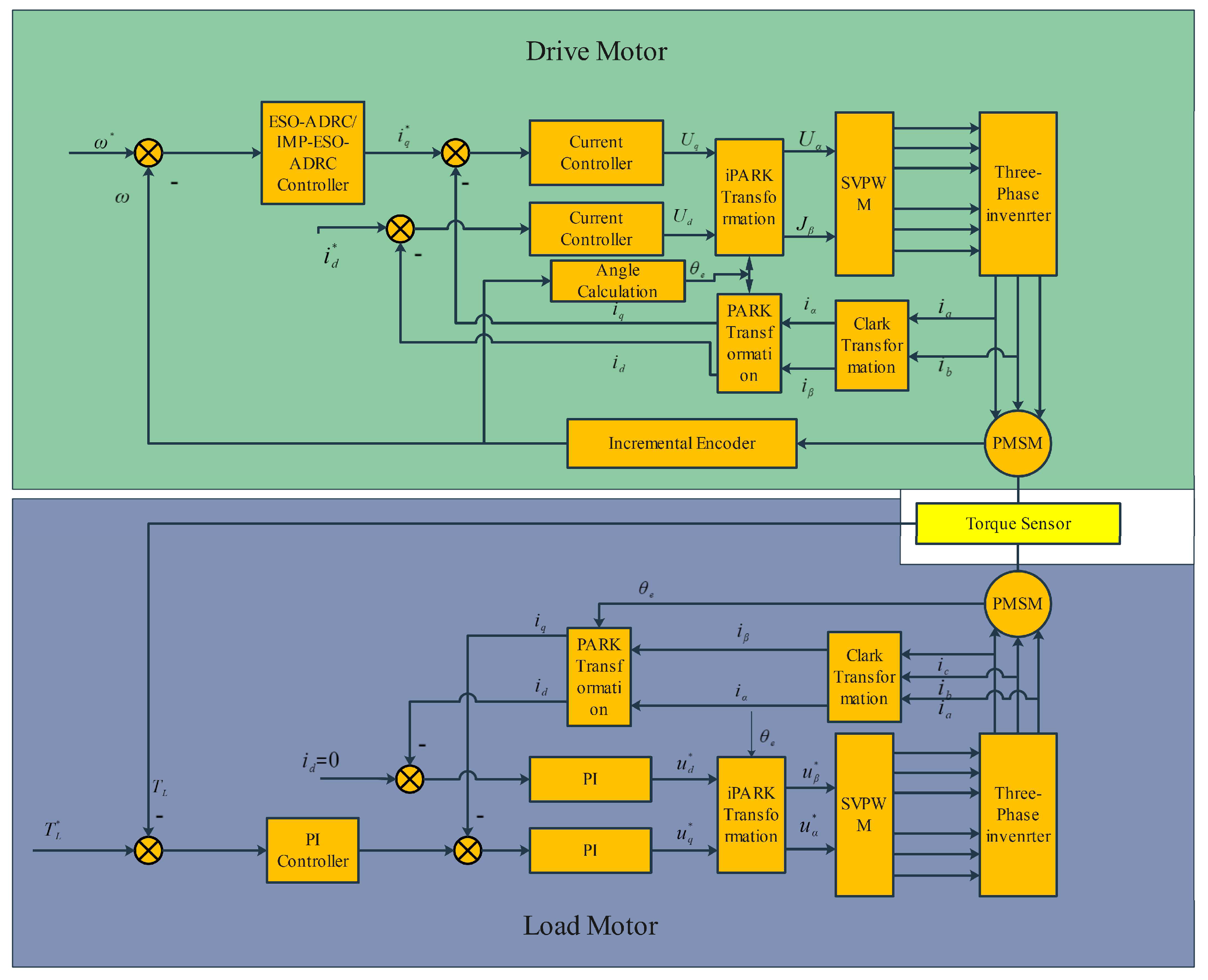
5.3. Experimental Results

In our research, experimental validation was conducted using an open-source multi-motor drive control comprehensive experimental platform. For specific details regarding the experimental platform, I recommend consulting ZhongKe ShenGu Technology Development Co., Ltd., Hefei City, Anhui Province, China. The cSPACE-RT OS control system, developed based on TMS320F28335 DSP and MATLAB/Simulink, encompasses three sets of motors for the towing platform (including high-performance torque sensors), motor drive control cabinets, and PC software. Figure 23 illustrates the servo control platform and the load system.

Table 5. Parameters of permanent magnet servo motor.

Rated voltage	24 V
Rated power	200 W
Rated speed	1500 RPM (Revolutions per minute)
Incremental encoder	2500 PPR (Pulses per revolution)

provides the parameters of the permanent magnet servo motors used in the experiment. The motor speed is obtained from the encoder. Harmonic disturbance testing was conducted separately for each algorithm.

As shown in the control block diagram of Figure 24, the driving motor is set to a constant speed, with a continuous external disturbance provided by the load motor. An incremental encoder is used to acquire the speed signal, and a torque sensor is used to acquire the disturbance signal when stable.

The rated load of the speed motor is 1.27 N·m. During the experimental procedure, a sine wave disturbance of 1 N·m amplitude and 100 rad/s frequency will be applied by the load motor at 5 s.

The drive motor was set to a speed of 1000 RPM. The observer parameters for IMP-ESO-ADRC are ${\omega }_{0-\mathrm{IMP}-\mathrm{ESO}}=1000;{\omega }_{n-\mathrm{IMP}-\mathrm{ESO}}=100$. The controller parameters of IMP-ESO-ADRC are ${\omega }_{c-\mathrm{IMP}-\mathrm{ESO}}=300$. The observer parameters for ESO-ADRC are ${\omega }_{0-\mathrm{ESO}}=1500$. The controller parameters of ESO-ADRC are ${\omega }_{c-\mathrm{IMP}-\mathrm{ESO}}=400$. Figure 25 illustrates the experimental test results.

Based on the experimental results shown in Figure 25, the IMP-ESO-ADRC noticeably mitigated the impact of external disturbances. Prior to disturbance application, the steady-state error of IMP-ESO-ADRC was $\pm 1.27\mathrm{RPM}$, while the traditional ESO-ADRC’s steady-state error was $\pm 2.03\mathrm{RPM}$. After disturbance application, the steady-state error of IMP-ESO-ADRC was $\pm 1.41\mathrm{RPM}$, while the traditional ESO-ADRC’s steady-state error was $\pm 5.37\mathrm{RPM}$. The improvement was significant. Therefore, based on the experimental results, it can be concluded that IMP-ESO demonstrated superior error tracking performance and stronger anti-interference capability.

6. Conclusions

This paper proposes a novel dynamic compensation method to estimate the states of linear systems with disturbance. By utilizing known information and online measurement information, an IMP-ESO (internal model principle-based expanded state observer) is designed that can be used for ADRC to simultaneously estimate disturbance and system states.

The EDO almost combines the advantages of ESO and IMP, possessing strong robustness against systems and disturbances, similarly to ESO in active disturbance rejection, while also proposing a feasible method to maximally utilize disturbance information, which was verified through simulations and experiments. Therefore, the proposed EDO has considerable universality. Compared with existing active disturbance rejection methods, this method can improve performance with smaller tuning gains when the interference contains non-constant disturbances. Meanwhile, large variations in the coefficients of the controlled system and IMP-ESO-ADRC parameters do not affect the stability of the closed-loop control system based on IMP-ESO-ADRC, fully demonstrating the strong robustness of the control system based on IMP-ESO-ADRC.

We only proposed the basic principles for observer design. In engineering applications, techniques such as transient response shaping would still require tuning. From a theoretical perspective, a systematic method of utilizing the prior dynamics of disturbances was provided. Future work involves utilizing measurement results online to calculate disturbance dynamics.

References

1. Han, J. From PID to active disturbance rejection control. IEEE Trans. Ind. Electron. 2009, 56, 900–906. [Google Scholar] [CrossRef]
2. Zolotas, A. Disturbance Observer-Based Control: Methods and Applications [Bookshelf]. IEEE Control Syst. Mag. 2015, 35, 55–57. [Google Scholar] [CrossRef]
3. Yin, X.; Shi, Y.; She, J.; Wang, H. Equivalent Input Disturbance-Based Control: Analysis, Development, and Applications. IEEE Trans. Cybern. 2023. [Google Scholar] [CrossRef] [PubMed]
4. Hao, Z.; Tian, Y.; Yang, Y.; Gong, Y.; Hao, Z.; Zhang, J. Sensorless Control Based on the Uncertainty and Disturbance Estimator for IPMSMs with Periodic Loads. IEEE Trans. Ind. Electron. 2023, 70, 5085–5093. [Google Scholar] [CrossRef]
5. Hezzi, A.; Elghali, S.B.; Bensalem, Y. ADRC Based Robust and Resilient Control of a 5 Phase PMSM Driven Electric Vehicle. Machines 2020, 8, 17. [Google Scholar] [CrossRef]
6. Sira-Ramirez, H.; Linares-Flores, J.; Garcia-Rodriguez, C.; Contreras-Ordaz, M.A. On the Control of the Permanent Magnet Synchronous Motor: An Active Disturbance Rejection Control Approach. IEEE Trans. Control Syst. Technol. 2014, 22, 2056–2063. [Google Scholar] [CrossRef]
7. Zurita-Bustamante, E.W.; Sira-Ramirez, H.; Linares-Flores, J. On the sensorless rotor position control of the permanent magnet synchronous motor: An active disturbance rejection approach. In Proceedings of the 13th International Conference on Power Electronics (CIEP), Guanajuato, Mexico, 20–23 June 2016; Volume 12, pp. 12–17. [Google Scholar]
8. Du, B.; Wu, S.; Han, S.; Cui, S. Application of Linear Active Disturbance Rejection Controller for Sensorless Control of Internal Permanent-Magnet Synchronous Motor. IEEE Trans. Ind. Electron. 2016, 63, 3019–3027. [Google Scholar] [CrossRef]
9. Zhiwang, C.; Zizhen, Z.; Jie, C.Y. Fal function improvement of ADRC and its application in quadrotor aircraft attitude control. Control Decis. 2018, 33, 1901–1907. [Google Scholar]
10. Han, J. Active disturbance rejection controller and its applications. Control Decis. 1998, 13, 19–23. (In Chinese) [Google Scholar]
11. Gao, Z. Scaling and bandwidth-parameterization based controller tuning. In Proceedings of the American Control Conference, Minneapolis, MN, USA, 14–16 June 2006; Institute of Electrical and Electronics Engineers (IEEE): New York, NY, USA, 2006; pp. 4989–4996. [Google Scholar]
12. Guo, B.; Bacha, S.; Alamir, M.; Mohamed, A.; Boudinet, C. LADRC applied to variable speed micro-hydro plants: Experimental validation. Control Eng. Pract. 2019, 85, 290–298. [Google Scholar] [CrossRef]
13. Guo, B.; Bacha, S.; Alamir, M. A review on ADRC based PMSM control designs. In Proceedings of the 43rd Annual Conference of the IEEE Industrial Electronics Society (IECON), Beijing, China, 29 October–1 November 2017; pp. 1747–1753. [Google Scholar]
14. Guo, B.; Bacha, S.; Alamir, M.; Boudinet, C.; Mesnage, H. An enhanced phase-locked loop with extended state observer. In Proceedings of the 20th International Symposium on Power Electronics (Ee), Novi Sad, Serbia, 23–26 October 2019; pp. 1–6. [Google Scholar]
15. Fareh, R.; Khadraoui, S.; Abdallah, M.Y.; Baziyad, M.; Bettayeb, M. Active Disturbance Rejection Controllers for robotic systems: A review. Mechatronics 2021, 80, 102671. [Google Scholar] [CrossRef]
16. Li, B.; Zhu, L. An Improved Fractional-Order Active Disturbance Rejection Control: Performance Analysis and Experiment Verification. arXiv 2021, arXiv:2112.05553. [Google Scholar] [CrossRef]
17. Mado’nski, R.; Herman, P. Survey on methods of increasing the efficiency of extended state disturbance observers. ISA Trans. 2015, 56, 18–27. [Google Scholar] [CrossRef]
18. Yang, X.; Huang, Y. Capabilities of extended state observer for estimating uncertainties. In Proceedings of the 2009 American Control Conference, St. Louis, MO, USA, 10–12 June 2009; IEEE: Piscataway, NJ, USA, 2009. [Google Scholar] [CrossRef]
19. Chen, W.-H.; Yang, J.; Guo, L.; Li, S. Disturbance Observer Based Control and Related Methods—An Overview. IEEE Trans. Ind. Electron. 2016, 63, 1083–1095. [Google Scholar] [CrossRef]
20. Spurgeon, S.K. Sliding mode observers: A survey. Int. J. Syst. Sci. 2008, 39, 751–764. [Google Scholar] [CrossRef]
21. Freidovich, L.B.; Khalil, H.K. Performance recovery of feedback-linearization-based designs. IEEE Trans. Autom. Control 2008, 53, 2324–2334. [Google Scholar] [CrossRef]
22. Wu, Y.; Isidori, A.; Lu, R.; Khalil, H. Performance recovery of dynamic feedback–linearization methods for multivariable nonlinear systems. IEEE Trans. Autom. Control 2008, 65, 1365–1380. [Google Scholar] [CrossRef]
23. Han, B. Optimization Strategies for Power and Load Control of Large Wind Turbines. Ph.D. Thesis, Hunan University, Changsha, China, 2019. [Google Scholar]
24. Mei, Z.; Li, C.; Xu, S. Resonance Frequency Detection Method of Servo Drive System Based on SOGI-FLL. Electr. Mach. Control Appl. 2023, 50, 74–80. [Google Scholar]
25. Huang, J. Nonlinear Output Regulation: Theory and Applications; SIAM: Philadelphia, PA, USA, 2004. [Google Scholar]
26. Herbst, G. Transfer Function Analysis and Implementation of Active Disturbance Rejection Control. J. Control Theory Appl. 2021, 19, 19–34. [Google Scholar] [CrossRef]
Figure 1. Control block diagram of ADRC based on ESO.
Actuators 13 00029 g001
Figure 2. Closed-loop control block diagram of ADRC based on IMP-ESO.
Actuators 13 00029 g002
Figure 3. Block diagram of ADRC closed-loop control principle based on IMP-ESO.
Actuators 13 00029 g003
Figure 4. Closed-loop control block diagram of IMP-ESO-ADRC.
Actuators 13 00029 g004
Figure 5. Closed-loop control block diagram of ESO-ADRC.
Actuators 13 00029 g005
Figure 6. Equivalent block diagram of ADRC closed-loop control.
Actuators 13 00029 g006
Figure 7. Bode plot of the closed-loop system based on parameters A and B-1.
Actuators 13 00029 g007
Figure 8. Bode plot of the closed-loop system based on parameters B-1, C1-1 and C1-2.
Actuators 13 00029 g008
Figure 9. Bode plot of the closed-loop system based on parameters B-1, C2-1 and C2-2.
Actuators 13 00029 g009
Figure 10. Bode plot of the closed-loop system based on parameters B-1, C3-1 and C3-2.
Actuators 13 00029 g010
Figure 11. Bode plot of the closed-loop system based on parameters A and B-2.
Actuators 13 00029 g011
Figure 12. Bode plot of the closed-loop system based on parameters B-2, D1-1, and D1-2.
Actuators 13 00029 g012
Figure 13. Bode plot of the closed-loop system based on parameters B-2, D2-1, and D2-2.
Actuators 13 00029 g013
Figure 14. Bode plot of the closed-loop system based on parameters B-2, D3-1, and D3-2.
Actuators 13 00029 g014
Figure 15. Comparison of input signal and output signal.
Actuators 13 00029 g015
Figure 16. Comparison of control error.
Actuators 13 00029 g016
Figure 17. Comparison of disturbance tracking.
Actuators 13 00029 g017
Figure 18. Comparison of disturbance tracking error.
Actuators 13 00029 g018
Figure 19. Comparison of input signal and output signal.
Actuators 13 00029 g019
Figure 20. Comparison of control error.
Actuators 13 00029 g020
Figure 21. Comparison of disturbance tracking.
Actuators 13 00029 g021
Figure 22. Comparison of disturbance tracking error.
Actuators 13 00029 g022
Figure 23. Open-source multi-motor drive control comprehensive experimental platform.
Actuators 13 00029 g023
Figure 24. Control block diagram.
Actuators 13 00029 g024
Figure 25. Experimental results.
Actuators 13 00029 g025