Abstract
Energy consumption is one of the most critical factors in determining the kinematic performance of quadruped robots. However, existing research methods often encounter challenges in quickly and efficiently reducing the energy consumption associated with quadrupedal robotic locomotion. In this paper, the deep deterministic policy gradient (DDPG) algorithm was used to optimize the energy consumption of the Cyber Dog quadruped robot. Firstly, the kinematic and energy consumption models of the robot were established. Secondly, energy consumption was optimized by reinforcement learning using the DDPG algorithm. The optimized plantar trajectory was then compared with two common plantar trajectories in simulation experiments, with the same period and the number of synchronizations but varying velocities. Lastly, real experiments were conducted using a prototype machine to validate the simulation data. The analysis results show that, under the same conditions, the proposed method can reduce energy consumption by 7~9% compared with the existing optimal trajectory methods.
1. Introduction
Quadruped robots, due to their excellent working ability in complex terrain and dangerous environments [1], have been widely used in rescue operations [2], military contexts [3], exploration missions [4], and mining activities [5], offering significant advantages such as low cost and high completion rates. However, the rapid depletion of energy reserves during locomotion remains a critical issue, resulting in short operating time. Reducing the motion energy consumption without losing the motion performance has become a key challenge to achieving longer operational duration and high-performance robot service.
Various methods, including gait planning [6,7,8], trajectory planning [9,10], and reinforcement learning [11,12,13,14,15], have been used to enhance the control of four-legged robots. Wang et al. proposed a soft gait control strategy that minimized tracking error and jitter to improve the quadrupedal crawling robot’s stable passage in a sidehill environment [6]. Li et al. proposed a gait-switching control method for quadrupedal robots based on the combination of dynamic and static and improved the robot’s ability to adapt to different terrains using Matlab–Adams co-simulation [7]. Chen et al. proposed a quadrupedal robot that was able to adapt to multiple terrains based on the idea of trajectory planning by combining the Cartesian space with the joint space [8]. Chen et al. proposed a quadrupedal robot that was able to adapt to multiple terrains based on the idea of trajectory planning by combining the Cartesian space with the joint space’s bionic foot trajectory [9]. Levin et al. reported on learning hand–eye coordination for robotic grasping through deep learning and big data [11]. Haarnoja et al. proposed a sample-efficient deep reinforcement learning (RL) algorithm based on maximum entropy artificial intelligence for real robots to learn to walk [12]. Tan et al. utilized deep reinforcement learning techniques to automate quadrupedal robots’ agile locomotion [13]. Nagabandi A et al. conducted a study on learning online adaptation in the context of model-based reinforcement learning to enable robots to learn to adapt to dynamic real-world environments through reinforcement learning [15]. Notably, the robot’s autonomous movement, recognition of the terrain to plan its path, etc., were realized by reinforcement learning. This shows that reinforcement learning methods have very high potential value.
The current conventional methods for studying robot energy consumption are as follows. Yang et al. proposed a trotting gait foot trajectory based on cubic spline interpolation and investigated the variation in energy consumption due to different gait parameters of the quadrupedal robot SCalf by simulation [16]. Benotsmane et al. found that an industrial robot executed three defined reference trajectories with reduced accuracy using an MPC controller, but was always faster and required less energy [17]. G. Wang et al. proposed a quadratic planning force-allocation controller to reduce the energy consumption of a hexapod robot by optimizing the instantaneous power at each time step [18]. Mikolajczyk et al. investigated the current state of the art of bipedal walking robots that use natural bipedal locomotion (humans and birds) as well as innovative synthetic solutions and probed the energy efficiency of bipedal robots [19]. These methods have made good progress in the control of legged robots. The feasibility of the traditional [19,20,21,22,23] approach can be directly observed since it usually uses different platforms for simulation, planning, and control, and the obtained data are imported into the robot control system for experiments. However, repeated attempts are inefficient and often accompanied by problems such as damage to the body, slow progress, and unsatisfactory results. Therefore, it is very difficult to consider the energy consumption with the traditional approach, and reinforcement learning can play an important role in this regard.
This paper focuses on the energy consumption of the legs of the Cyber Dog quadruped robot during locomotion. To optimize the energy consumption, reinforcement learning was performed using the deep deterministic policy gradient (DDPG) algorithm, the optimal energy consumption data were extracted in a simulated environment, and then the energy consumption of the robot was compared with that of two common foot end trajectories [9] under the same experimental conditions. The power output of each joint of the robot’s leg was reduced while maintaining the speed of movement, thus optimizing energy consumption under the same conditions. The paper is structured as follows. Section 2 models the robot’s kinematics and energy consumption and analyzes two common end-of-foot trajectories. Section 3 describes the experimental methodology and setup to lay the research foundation for subsequent experiments. Section 4 compares the optimal end-of-foot trajectories obtained through reinforcement learning with the conventional end-of-foot trajectories and compares the energy consumption at the same speed, period, and number of synchronizations through simulation experiments. The reliability of the simulation results was confirmed by prototype experiments. The results obtained from the study are used in Section 5 to evaluate the advantages of the discussed methods. Finally, concluding remarks are made, and future research directions are outlined. The method in this paper can reduce the energy consumption in the movement of quadrupedal robots, extend the endurance of quadrupedal robots in complex and dangerous environments, and reduce the risk of accidental injuries caused by experiments with high-value robots in real environments.
2. Robot Modeling
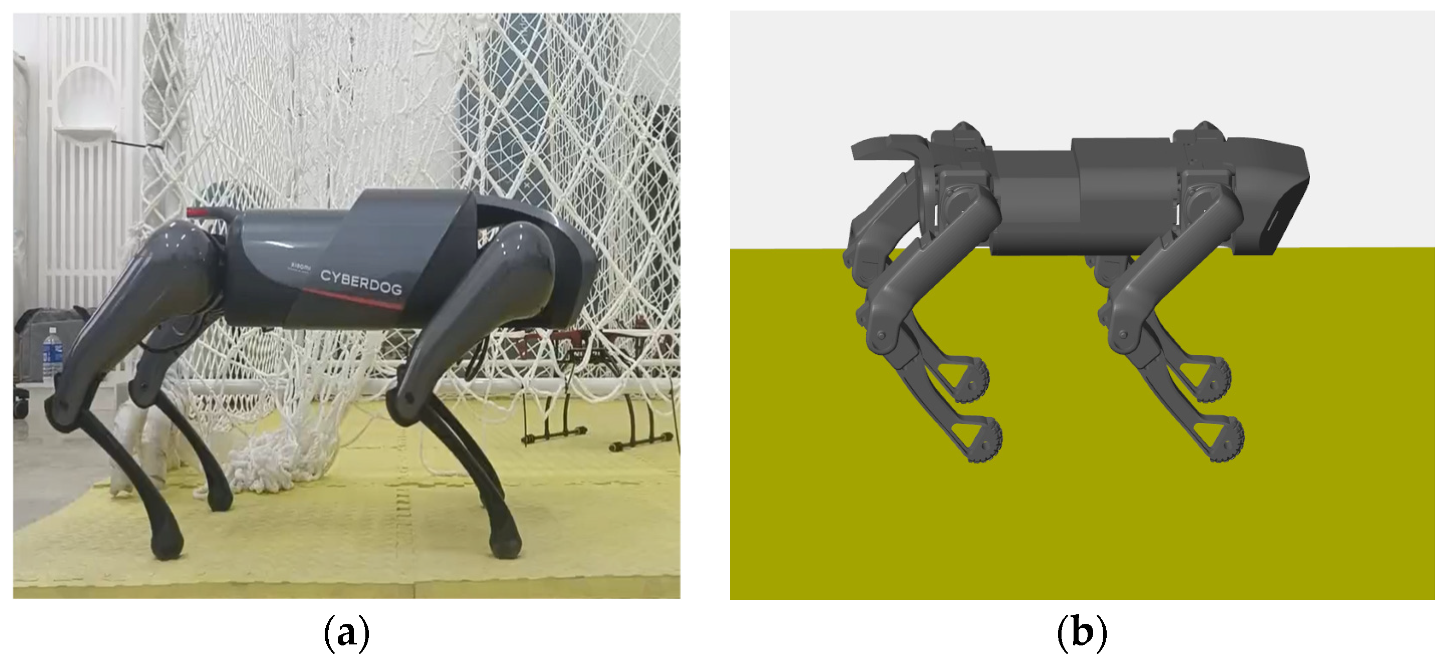
The Cyber Dog quadrupedal robot is an in-house prototype developed by Xiaomi equipped with three degrees of freedom in each leg and high-performance servo motors. These motors provide a maximum output torque of 32 Nm and a maximum speed of 220 rpm, allowing the robot to move at speeds of 3.2 m/s. The Cyber Dog’s design ensures high-torque and high-speed performance with a fast response. The robot is further equipped with the NVIDIA JETSON XAVIER NX platform, which integrates 384 CUDA cores, 48 Tensor Cores, six Carmel ARM CPUs, and two deep learning acceleration engines for fast interaction between simulation data and real prototypes. The training platform was based on the Matlab simulation platform Simulink, and the 3D diagram of the Cyber Dog quadruped robot was imported into the Simulink simulation platform to establish the intelligent body simulation system. The system meets the simulation requirements, such as joint limitation and ground contact, and has the ability of reinforcement learning.
In order to better train for energy optimization in simulation, the following assumptions were adopted:
The study focused only on the motion of the robot on the plane and ignored the friction between the joints.
The rolling motion of the robot’s hip joints was not considered when walking on a plane.
Considering these preconditions, Matlab configured the external environment parameters for the intelligent body to interact with Simulink. The model contained 111 observations, including the Cartesian coordinates of the torso, the orientation, the joint angles, the 3D velocities, the angular velocities, the joint velocities, and the joint moments. This facilitated a more consistent setup of reward terms in the reward function, consistent with the research described in this paper. For this paper, the dimensions of the simulated robot were aligned with those of the real-world robot to improve the accuracy of the simulation. Furthermore, the fidelity of the physics simulator was enhanced by carefully tuning the parameters of the robots in the simulation, such as the joint rotation ranges and motor control ranges. Figure 1a,b illustrate the real and simulated models.
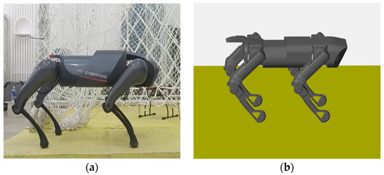
Figure 1.
Cyber Dog quadruped robot: (a) Cyber Dog quadrupedal robot prototype; (b) Cyber Dog quadruped robot simulation model.
2.1. Kinematics Modeling
2.1.1. Swing Phase of Leg Mechanism
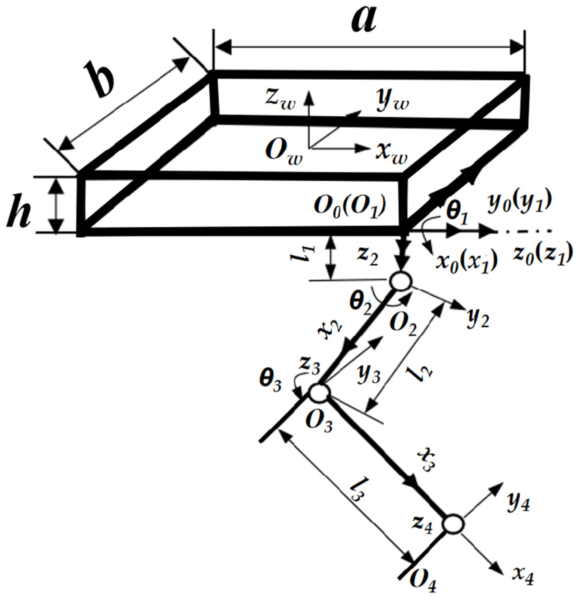
A body coordinate system (Ow, −xw, yw, zw) was established on the quadruped robot; Ow is the coordinate origin at the center of the torso of the robot model. The leg mechanism can be regarded as a series of connecting rods constituting a connecting rod mechanism in each joint of the leg to establish the connecting rod coordinate system (Oi, −xi, yi, zi) with i = 0, 1, 2, 3, and 4, as shown in Figure 2.
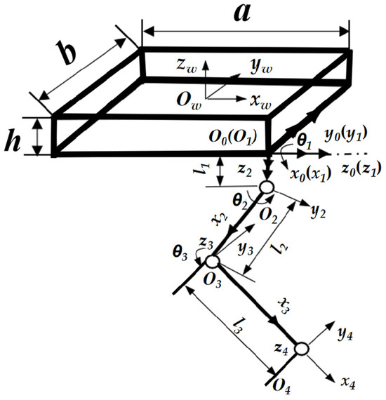
Figure 2.
Simplified diagram of the right front (RF) leg swing mechanism.
θ1, θ2, and θ3 denote the joint angles of each joint in the leg mechanism; l1, l2, and l3 denote the lengths of each connecting rod of the leg mechanism. The Denavit–Hartenberg (D–H) parameters for when the leg mechanism was in the swing phase are detailed in Table 1.

Table 1.
D–H parameters for the swing phase of the right anterior (RF) leg mechanism.
Using the homogeneous matrix to represent the spatial posture of each joint of the leg, the kinematic equation for the swing phase is Equation (1):
where s23 = sin(θ2 + θ3), c23 = cos(θ2 + θ3), si = sinθi, and ci = cosθi.
Px, Py, and Pz, which can be obtained from Equation (1), are the origin vector elements of the position of the foot end relative to the basic coordinate system, and they are expressed in Equation (2).
The inverse transformation of the chi-square matrix [7] is used to obtain the transformation equation of the foot end position with respect to the angle of the joint associated with the lateral swing θsw1, the angle of the thigh joint θsw2, and the angle of the calf joint θsw3, as shown in Equation (3):
where .
2.1.2. Supporting Phase of Leg Mechanism
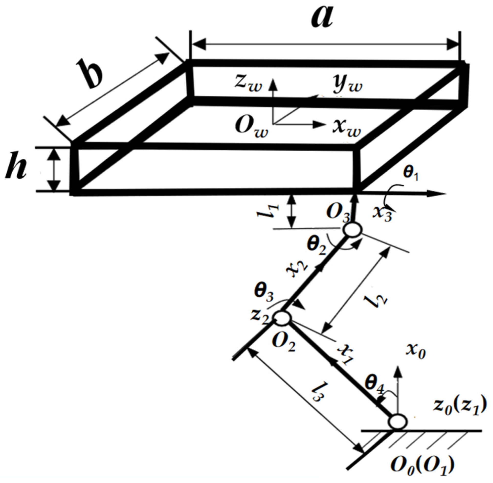
When the leg mechanism is in the support phase, there is no side swing motion; therefore, the θ1 of the side swing joints is constant at zero. The spatial coordinate system of each joint of the leg in this phase is shown in Figure 3. The θ2, θ3, and θ4 denote the joint angles of the shoulder, knee, and ankle joints, respectively. In addition, the D–H parameters of the supported phase are shown in Table 2.
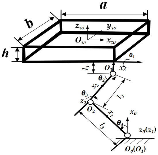
Figure 3.
Simple diagram of right front (RF) leg support mechanism.
Table 2.
D–H parameters for the support phase of the right front (RF) leg mechanism.
Then the kinematics equations of the supported phase are expressed in Equation (4).
Px, Py, and Pz, derived from Equation (4), are the origin vector elements of the foot’s end phase with respect to the position of the base coordinate system when the leg mechanism is in the support phase; they are expressed in Equation (5).
The inverse transformation of the chi-square matrix was used to obtain the transformation equation θ2sp, θ3sp for the foot-end position with respect to the angle of the transverse support related to the knuckle, as shown in Equation (6).
where .
The kinematic inverse solution provided a theoretical basis for the subsequent programming of the control system in the Matlab simulation by obtaining the variables of each joint.
2.2. Energy Model
To analyze the energy consumption of the Cyber Dog, it was necessary to establish an energy consumption model. For the energy consumption of the Cyber Dog in this paper, only the mechanical power was considered, so the calculation of energy consumption was obtained by integrating the mechanical power into the gait cycle, where power is the product of joint moment and joint angular velocity. This is shown in Equation (7), where T is the gait cycle, E is the energy consumption in one gait cycle, and P is the joint power. In this paper, the dynamics of the robot are not considered; the joint moments and joint angular velocities of the robot can be observed, and the data were obtained by the oscilloscope module in Simulink.
In the second line of Equation (7), i is the i-th leg of the quadruped robot, j is the j-th joint of the quadruped robot, τ is the quadruped robot’s joint moment, and is the angular velocity of the quadruped robot’s joints.
2.3. Foot Trajectory Analysis
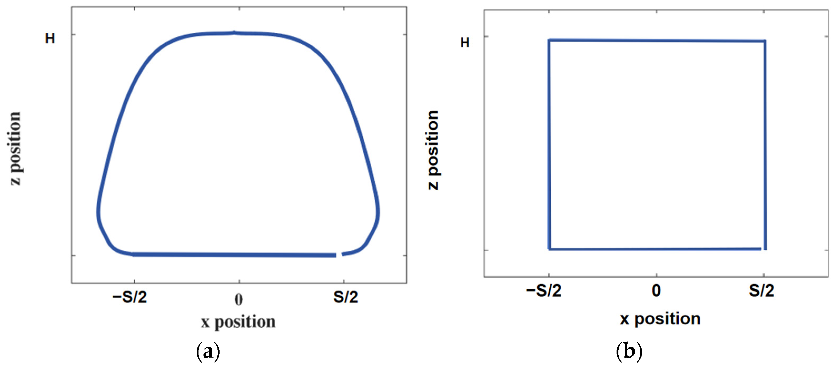
A well-designed foot-end trajectory can reduce joint moments and angular acceleration, reduce energy consumption, and increase the energy consumption rate. The composite pendulums and linear foot trajectories, commonly used foot trajectories, and the end-of-foot trajectory of a robot walking one step read by the Simulink oscilloscope module, as shown in Figure 4, were compared with the trajectories obtained from subsequent simulations of energy consumption. The gait parameters considered were S = 0.2 m, T = 0.8 s, and H = 0.15 m, which represent the displacement of the robot’s X-axis walking in one gait cycle, the gait period, and the maximum height of the robot’s foot lift in the Z-axis direction, respectively. In this paper, the side swing motion of the leg mechanism of the quadruped robot was not explored, so the motion of the foot end in the y-axis direction was not considered.
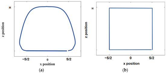
Figure 4.
Two common plantar trajectories: (a) composite pendulum foot trajectory; (b) straight line foot trajectory.
3. Methods
RL, the experimental method of this paper, is generally regarded as a process run by a Markov decision process (MDP), which is composed of the element groups {S, A, P, R, }. S = S1, S2 … St are the state sets, which are the sets of all states that the MDP can have. As shown below, the state St at any moment is a specific state in the state set s, where st = s, s ϵ S. A is the set of all behaviors that the actors can perform. Finally, P (st+1|st, at) represents what a given agent performs at time step t, and ∈ (0, 1) is the discount factor. Although P (st+1|st, at) is usually a complex, high-dimensional unknown task, samples can be collected through simulation or in the real world, and R (st, at) is the reward value obtained by st when the agent performs the action of at. A policy in RL is defined as the mapping from the state space to the operation space. In the strategy search, the goal is to find the optimal strategy π to maximize the long-term expected reward:
where
where Qπ(s) is the state distribution under policy π, that is, the probability of accessing state S under policy π, and Qπ (st, at) is the state action value function for calculating state action pairs. From st+1 to P (st+1|st, at) and to π(at|st) and t are terminal time steps. The reward function in reinforcement learning is as follows, which includes speed stability, straight walking, trunk vibration deviation, keeping forward and energy consumption, to encourage the robot to achieve the expected training results more quickly.
where is the quadruped robot’s reward for training while maintaining its speed, is the real-time velocity of the robot’s motion, is the velocity that the robot motion needs to reach, and A is the weighting factor for the velocity term. is the deviation of the fuselage in the y direction, which is related to whether the fuselage can walk in a straight line; B is the weighting factor of the y-axis offset term. represents the z-direction offset of the quadruped robot’s trunk during the movement, and C is the weight factor of the fuselage z-direction offset term. in order to maintain the training time of the quadruped robot, Ts is the sampling time of the environment, Tf is the simulation time of the environment, and D is the weighting factor for the keep-moving incentive term. is the energy consumption of the quadruped robot, where the environmental simulation time is 10 s, so the integral range is 0–10; the coefficient E is the weighting factor for the energy consumption incentive item. Each of the weighting coefficients A, B, C, D, and E needs to be obtained through subsequent simulations.
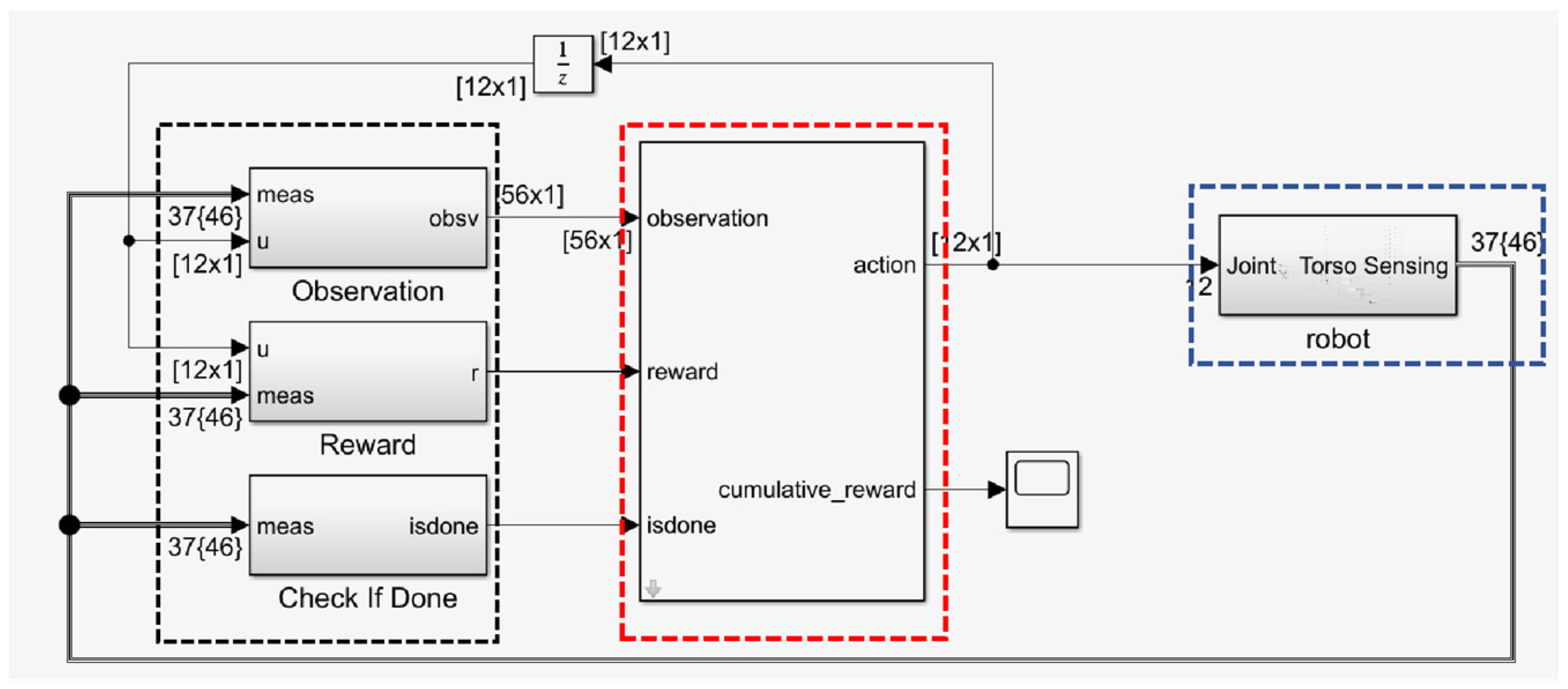
Considering the challenges of concurrently optimizing the quadrupedal robot’s speed of motion, straight-line walking, and energy consumption, which involve complex and difficult training, extended time requirements, and the risk of converging to the local optimal solution, this study divided the learning process into two stages. The first stage employed the DDPG algorithm to train the quadrupedal robot to maintain a stable speed and direction of motion. This was achieved by pruning the double-q learning, delaying the update of the goal and policy networks, and implementing goal policy smoothing to avoid overestimating the value function; the energy consumption term was not considered at this time, so the energy consumption term weighting factor E = 0. The second phase used the same DDPG algorithm to maintain stable motion on the basis of the linear motion of the quadruped robot while minimizing energy consumption. One notable advantage of this approach is that it provides faster simulation speeds, reduces experimental bias, and ensures that the robot is simulated with minimal energy consumption under ideal conditions. The reinforcement learning flowchart is shown in Figure 5; according to the joint moments and joint angular velocities fed back by the robot, the intelligent body unfolded its actions after intelligent decision-making and obtained feedback about the previous moment’s behavior, i.e., reward, from the changing state, which guided the subsequent behavioral decisions. Observations and actions for reinforcement of learning are shown in Table 3.
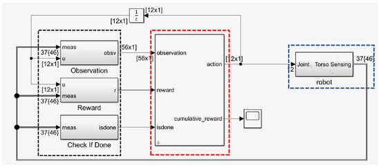
Figure 5.
Simulink reinforcement learning flowchart. The black box is the module of the environment state and reward function observed by the RL Agent, the red box is the module of the RL Agent, and the blue box is the module of the environment, i.e., the quadruped robot system simulated in this paper.
Table 3.
Observation and action content for reinforcement of learning.
The training was performed on a Matlab-based training platform with the Cyber Dog quadruped robot model. The model parameters were consistent with the body and joint sizes of a real quadruped robot. Two participant networks and two critic networks were used for the training network. The participant and critic networks consisted of three fully connected hidden layers with 128 neurons each and used the ReLU activation function. Furthermore, the algorithm was implemented using 10 random seeds, and details of the other training parameters are shown in Table 4.
Table 4.
Training environment parameters.
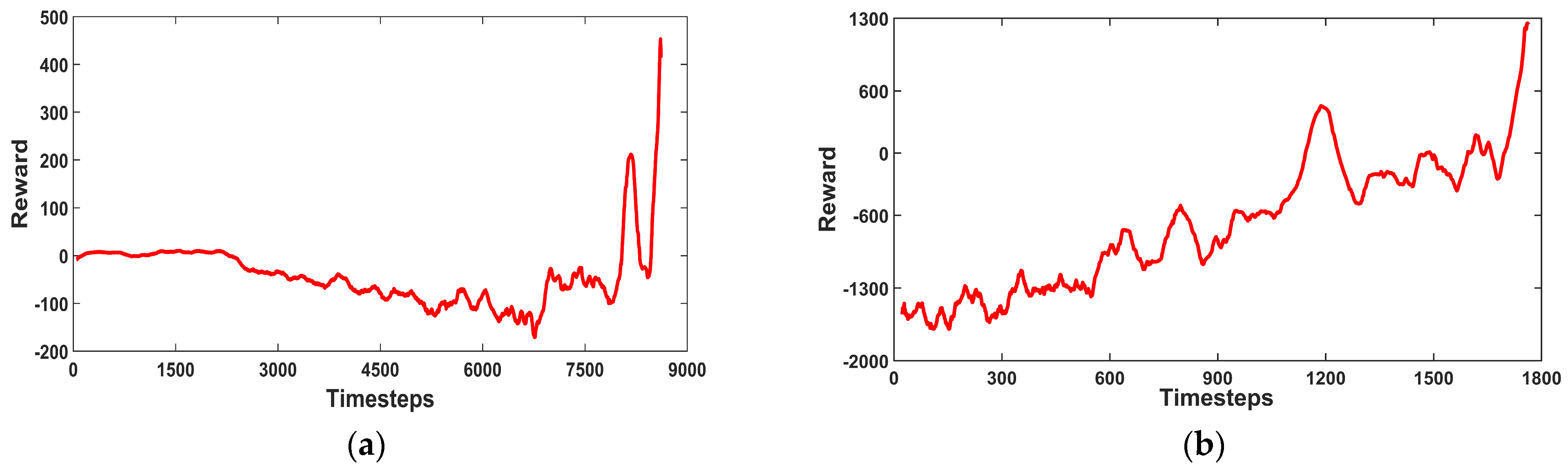
The results of continuous reinforcement learning were used to correct the reward function parameters. This yielded weighting coefficients A, B, C, D, and E of −2, −20, −50, 25, and −0.2 for each reward term, respectively. Thus, the robot could keep walking in a straight line, and the energy consumption reached the optimal state of the reward function in Equation (11); the reward function curve is shown in Figure 6.
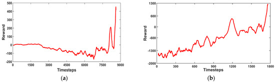
Figure 6.
Reinforcement learning reward function curves: (a) reward function curve in the first stage; (b) reward function curve in the second stage. The range of values of rt is .
The training process in Figure 6 shows that the energy consumption of the quadruped robot at this time is theoretically the optimal cycle that RL thinks can consume the least energy and maintain the speed of stable walking.
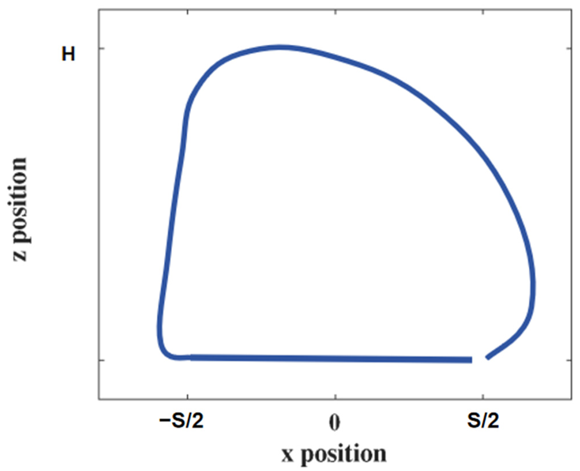
A theoretical analysis of the energy-optimal motion state of a quadruped robot can be performed using reinforcement learning. However, due to the autonomous nature of the learning process, effective gait cycles cannot be established. The method used in this paper was to extract the simulation data with the minimum energy consumption from the cycle with the optimal reward function, add the transform sensor module in Simulink, and connect it to an oscilloscope to observe the changes in the x and z coordinates of the robot’s foot-end. The foot-end trajectory record with the smallest energy consumption was extracted as the foot-end trajectory of the simulated trajectory, and the obtained trajectory is shown in Figure 7.

Figure 7.
Simulation of foot-end trajectories.
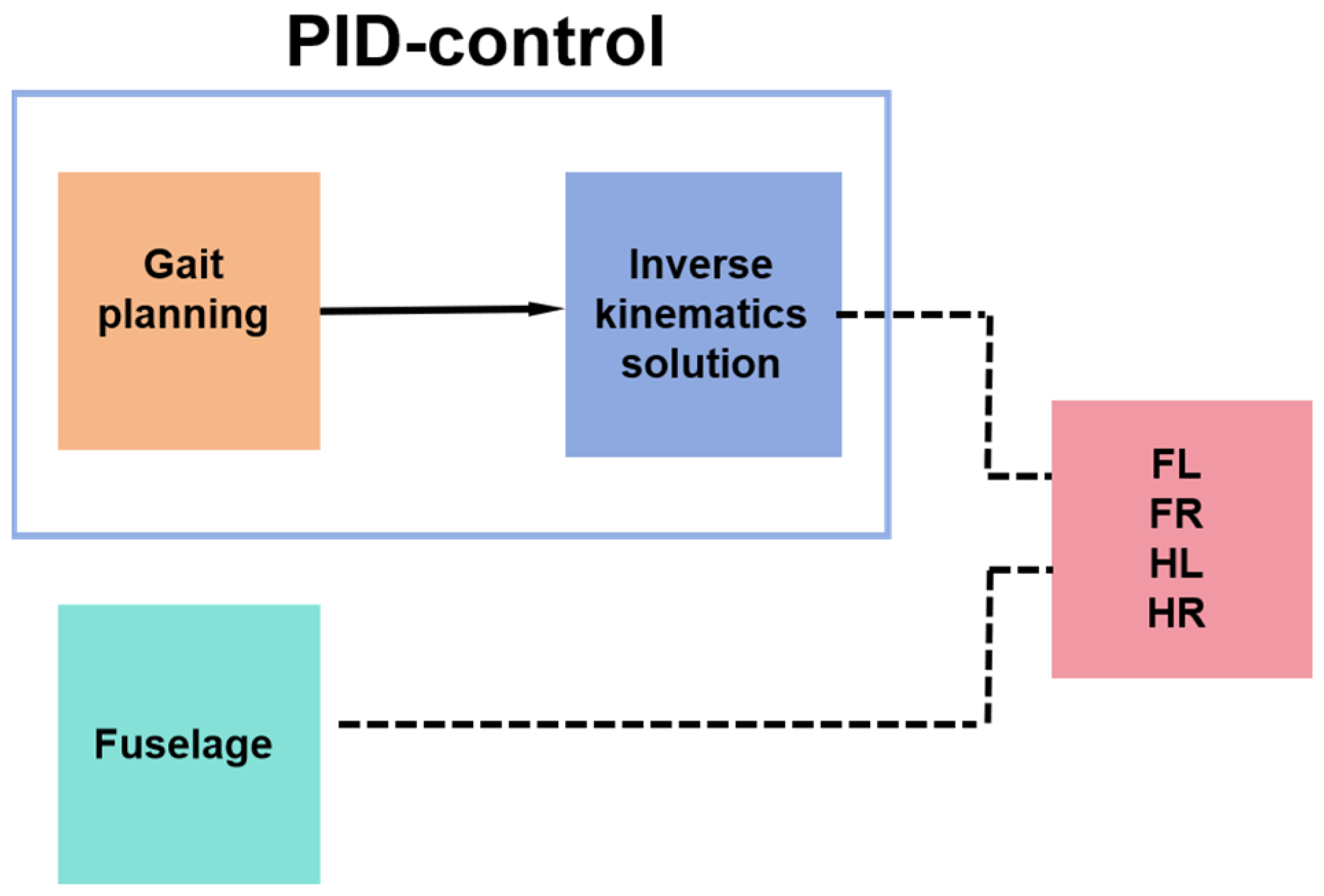
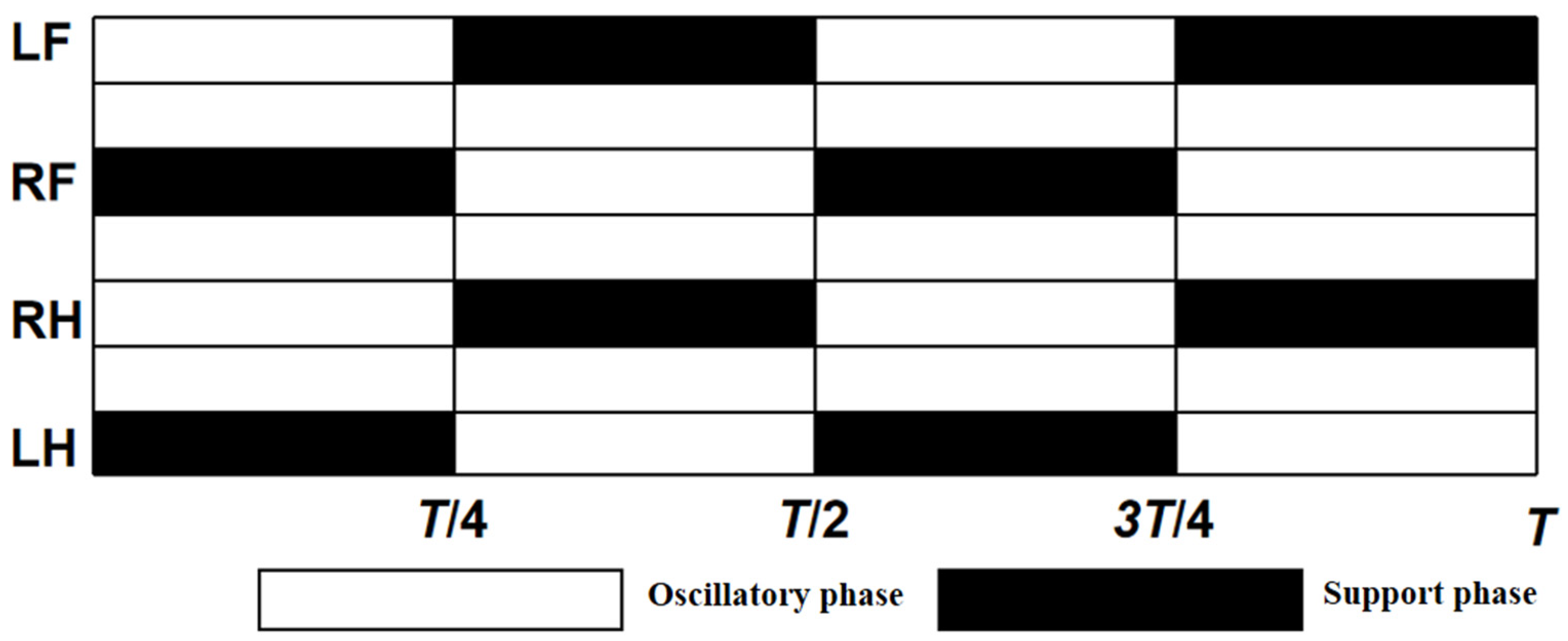
The kinematic inverse Equations (3) and (6) were implemented within the Simulink function module by Matlab. Then, the spatial position coordinates x, y, and z of the three foot-end trajectories were imported into the simulation system for simulation. An oscilloscope was connected to the joints to record the joint moments and angular velocities, and the difference in energy consumption between the simulated foot-end trajectories and the above trajectories at the same period and velocity can be calculated using Equation (7). For the control of the position and pose of the robot, PID control was used, and the control was built using Simulink in Matlab, as shown in Figure 8. The gait planning in the PID control used a diagonal gait, as shown in Figure 9, where the left front leg, right front leg, right hind leg, and left hind leg of the robot are divided and denoted by LF, RF, RH, and LH; the white squares represent the lifting of the leg in the swing phase, and the black squares represent the landing of the leg in the support phase, where T is the gait period, which was set to 0.8 s in this experiment. The equation for the relationship between the body velocity v and the step length S and the foot-end period Tm is as follows: , where Tm is the period of 0.2 s for one step of foot-end walking.

Figure 8.
Flowchart of PID control for quadruped robot.
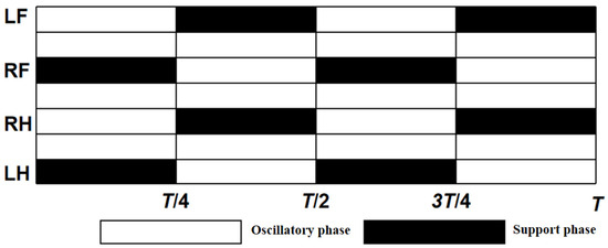
Figure 9.
Diagonal gait step sequence diagram.
4. Result and Discussion
In this section, simulation and prototype experiments are performed to compare the energy of the simulated foot-end trajectories with two common plantar trajectories at the same period and velocity, and the results of the experiments are discussed.
4.1. Simulation Experiment
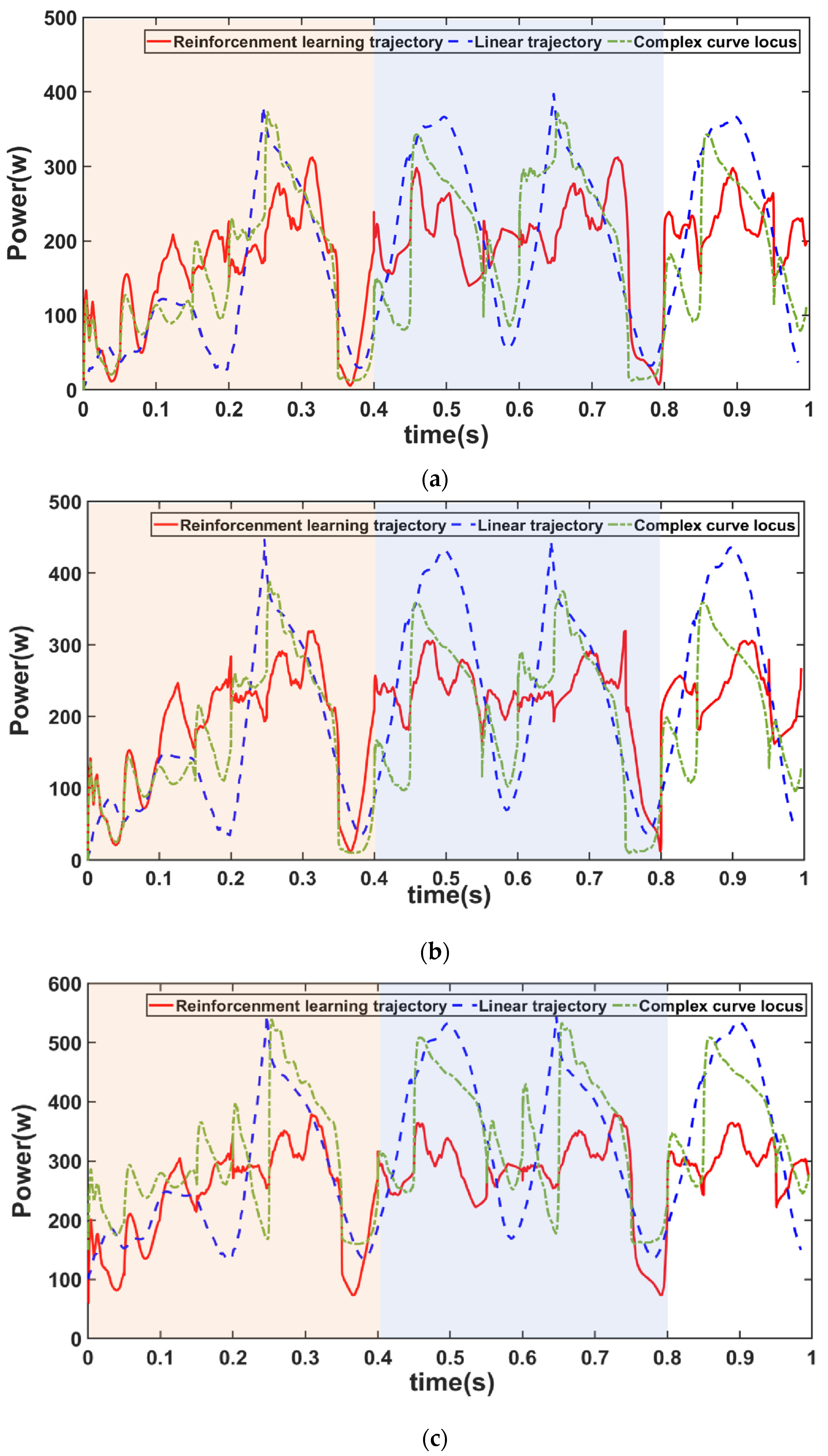
The experimental setup had a gait period of 0.8 s, divided into a support phase and a swing phase, each with a duration of 0.4 s. Figure 7 demonstrates the comparison of the robot movement power consumption with different plantar trajectories at three different speeds, 1 m/s, 1.2 m/s, and 1.4 m/s, within the same motion time. It can be seen that the simulation trajectory did not have obvious peak fluctuations in one gait cycle, and the change in the power was much more stable; the other two trajectories both had obvious sudden changes in the power at the moments of the interaction between the swing phase and the support phase, which exacerbated the energy consumption. Figure 10 shows that the simulated foot trajectory was more competitive than other common foot tracks, along with the power of the composite cycloid foot trajectory and the straight foot trajectory at three different speeds. The energy consumption in different cases was obtained by the calculation of Equation (7), and the energy reduction of this paper’s method over the other two common foot ends at different speeds was calculated by Equation (12), as shown in Table 5. It shows that the end-of-foot trajectories with velocities of 1 m/s, 1.2 m/s, and 1.4 m/s reduced the energy consumption by 9% to 12% compared with the other two trajectories. However, the ability to reduce energy consumption diminished with increasing speed. This may be due to the need to further optimize the joint moments and joint angular velocities for high-attitude motion states as the robot moves faster.
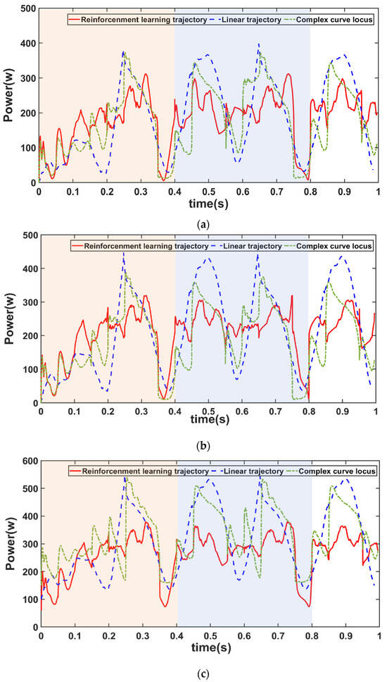
Figure 10.
Power consumption comparison of the three trajectories at a speed of (a) 1 m/s; (b) 1.2 m/s; (c) 1.4 m/s, where 0~0.4 s is the first cycle and 0.4~0.8 s is the second cycle.
Table 5.
Energy consumption of three foot trajectories (kJ) at speed.
In Equation (12), Emin is the energy consumption value of the other two foot-end trajectories with less energy consumption during the movement, Es is the energy consumption value of the simulated foot-end trajectory during the movement, and Dt is the energy consumption reduction.
4.2. Prototype Experiment
In contrast to simulation environments, real-world environments have a multitude of disturbances, such as joint friction and varying environmental conditions. Hence, it is important to validate the methodology presented in this paper by testing it on a physical prototype. In order to evaluate the difference between the direct data obtained from the simulation and the data obtained in the real environment, the data obtained from the simulation was integrated into the Cyber Dog quadruped robot.
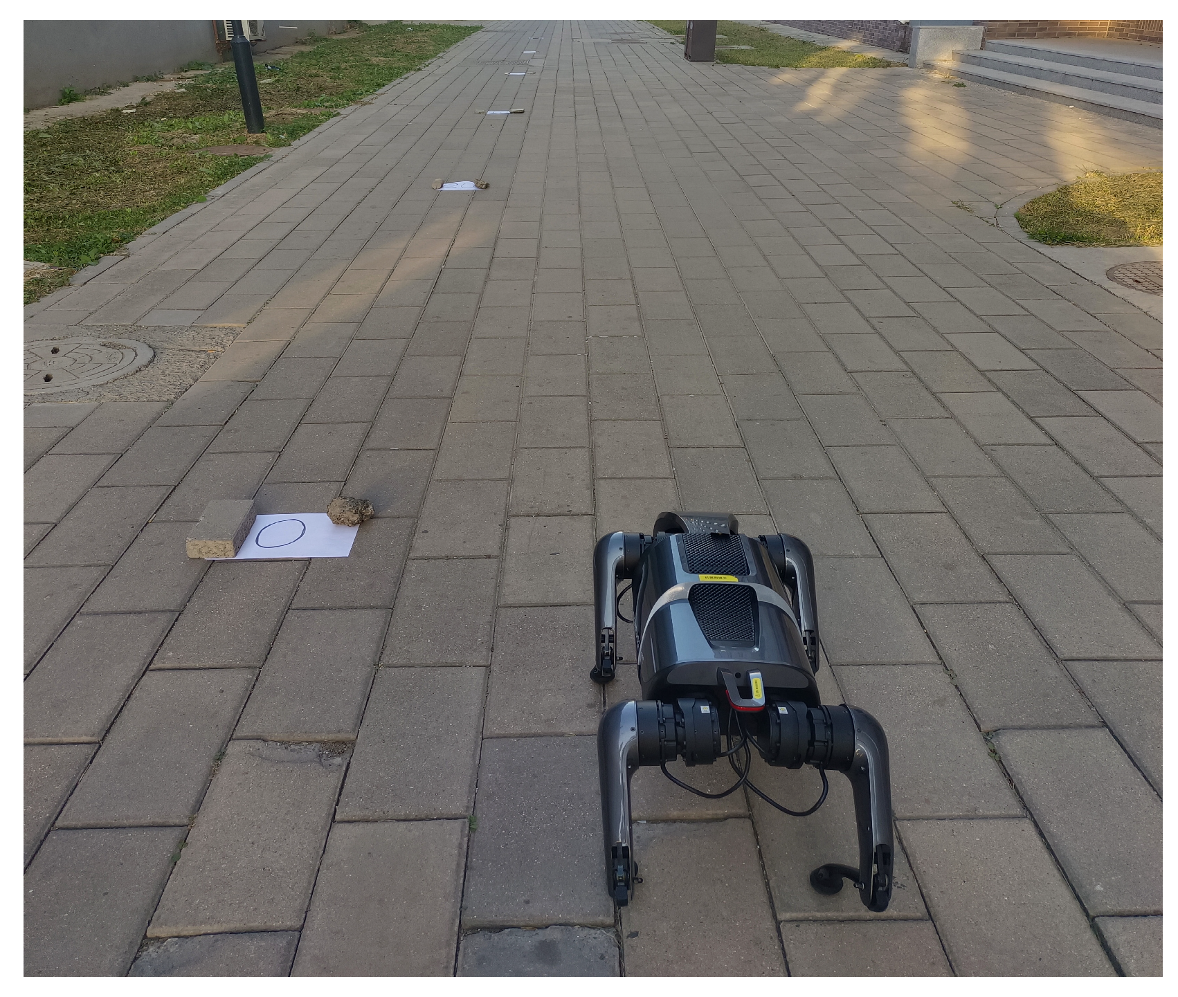
A 150-meter-long plane was chosen as the experimental area. The environmental variables were identical to the simulated environment. As shown in Figure 11, cue cards were placed every 10 m in the experimental area in order to measure the stability of the robot’s movement speed. The simulation data were transferred through the Type-C interface of the Cyber Dog. An energy consumption experiment was conducted during 100 m of robot travel using three different trajectories—a simulated trajectory, a compound pendulum trajectory, and a straight-line trajectory—and comparing the energy consumption of the robot on the basis of the level of power drop on the controller board.

Figure 11.
Experimental environment for real prototype movement.
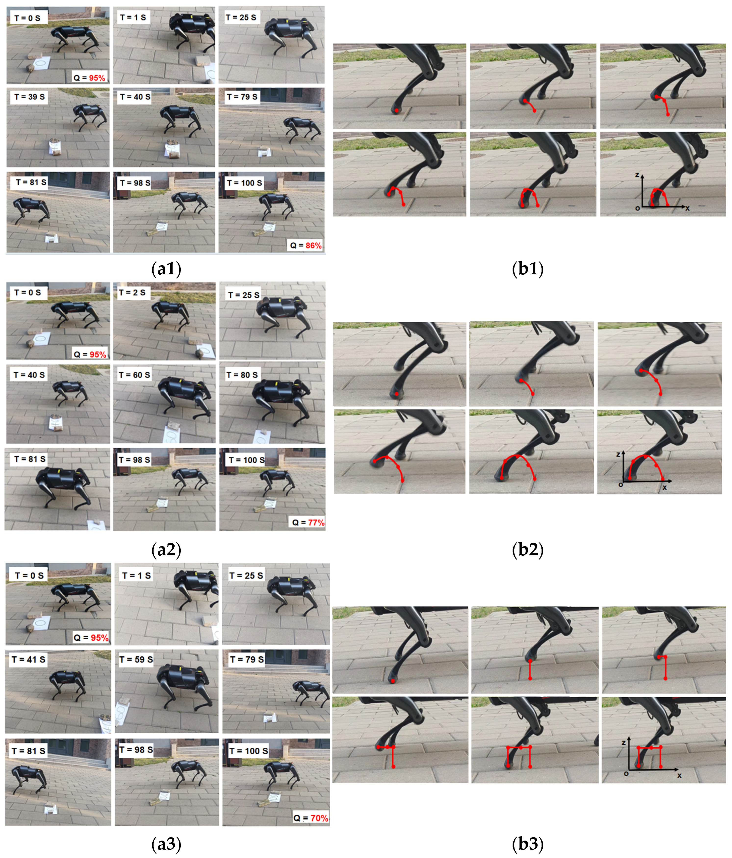
The robot was placed in the experimental environment and tasked with walking 100 m at a speed of 1 m/s. Comparison experiments on power consumption were conducted using different foot trajectories, and the position variations of the robot’s left forelimb (LF) foot were recorded during a gait cycle; the results are shown in Figure 12.

Figure 12.
Screenshots of Cyber Dog walking with different plantar trajectories in a real environment and the trajectory motion of the corresponding plantar trajectories in one cycle: (a1) Cyber Dog screenshot of the robot simulation trajectory walking experiment; (b1) real prototype: simulation trajectory diagram; (a2) Cyber Dog screenshot of the robot composite cycloid trajectory walking experiment; (b2) real prototype: composite cycloid trajectory diagram; (a3) Cyber Dog screenshot of the robot’s linear trajectory walking experiment; (b3) real prototype: straight line trajectory diagram. In the figure, T is the robot movement time and Q is the robot power consumption.
As evident from the experimental results in Figure 12, the power consumption in the real experiment with a simulation trajectory at a speed of 1 m/s was only 9%, which is significantly lower than the 18% power consumption with the composite pendulum trajectory and the 25% power consumption of the linear trajectory. In comparison with the higher power consumption of the composite pendulum trajectory, the simulated trajectory reduced the energy consumption by 9%. It is worth noting that the simulation results of the experiments conducted at a speed of 1 m/s showed that the energy consumption can be reduced by 12% using the method of this paper, but the results of the real experiments showed that the method of this paper can reduce the energy consumption by 9%, and the comparison revealed that there was a 3% error amplitude between the simulation and the real experiments, which may be attributed to the omission of factors such as the robot’s thermal power and joint friction loss in the energy consumption calculations. Considering that the value of the battery’s power display is not reliable, but there may be display errors, the experiment was carried out after using a multimeter to measure the battery’s voltage at the end of each charge to make it equal to 25 V to ensure that the robot consumed the same amount of energy during the experiment. The Cyber Dog could walk 3600 m at 1 m/s using a composite pendulum foot-end trajectory in a fully charged state. Using the foot-end trajectory simulated in this paper to move at 1 m/s at full power, the Cyber Dog could walk 3924 m, which is an increase of 324 m in walking distance, and significantly improved the robot’s endurance in complex and changing environments.
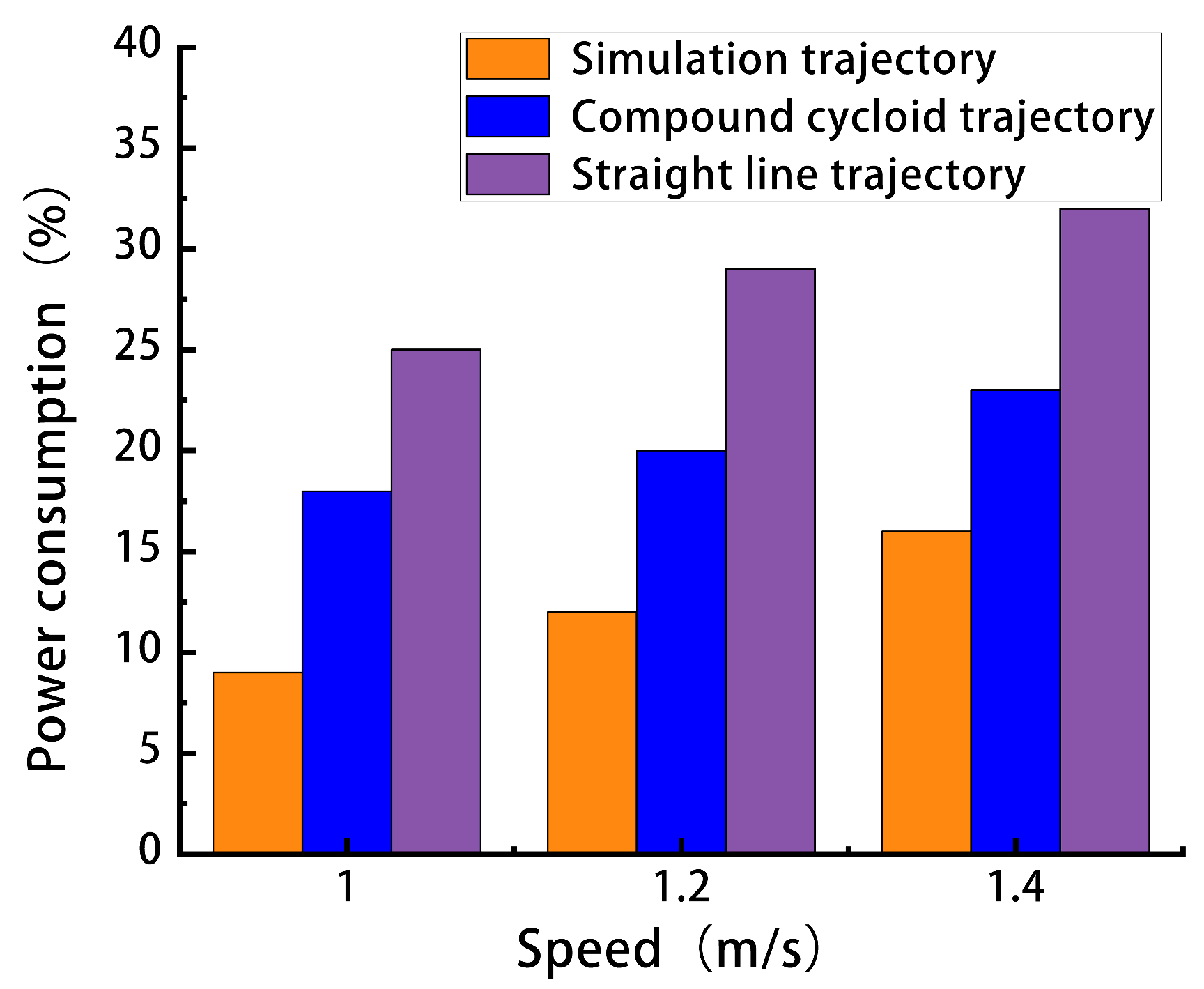
Then, the walking speed of the robot was adjusted to 1.2 m/s and 1.4 m/s for 100 m walking experiments. The magnitude of energy consumption was obtained by comparing how much battery power was consumed by the operator panel for different foot trajectory movements at different speeds, calculated with Equation (13). Subsequently, experiments were conducted to compare the power consumption of the robot when moving with three different foot-end trajectories at varying speeds. The results are shown in Figure 13.
where Ef is the initial power, En is the remaining power after movement, Pc is the power consumption of the robot, and the initial power is 95%.

Figure 13.
Comparison results of power consumption of different foot tracks at three speeds.
The comparative analysis of energy consumption at three different speeds revealed that the simulated trajectory consumed less energy than the other two trajectories. The energy consumption of the Cyber Dog quadrupedal robot increased with the speed of motion in a trend, consistent with the simulation results. Under the experimental conditions in this paper, the simulated trajectory achieved energy savings of 7% to 9% compared with the two common plantar trajectories, and the margin of error between the simulation and the real experiment was 3%. These simulation results are consistent with the experimental findings, thereby validating the effectiveness of the method proposed in this paper.
4.3. Discussion
Compared with the energy consumed by the two common plantar trajectories at varying velocities, the proposed method consistently resulted in lower overall energy consumption for the quadrupedal robot at the same velocity. This may be attributed to the finer control of joint motors by the RL intelligent body, which enabled the output of smaller joint moments and joint angular velocities while maintaining the velocity in order to reduce the power of the various joints of the quadrupedal robot at each moment. Further optimization of robot energy consumption using reinforcement learning can explore aspects like friction energy consumption between joints, joint onset angle, and foot lifting height. These factors can improve the energy efficiency of the legged robot and enhance the endurance of the robot. The method in this paper allows for training in a simulated environment, preventing the robot from accidental damage during training, and reducing resource wastage, which is of vital significance for high-value robots.
It is worth noting that legged and footed robots require different motion postures under different working conditions, which have been rarely studied by reinforcement learning. Particularly, the study of energy consumption in the robot’s high-posture motion is one of the key focal points for future research. Furthermore, robots with different morphologies may have different consumption for energy. It is intriguing to explore the application of reinforcement learning for optimizing the energy consumption of robots with different morphologies.
5. Conclusions
The following conclusions can be made through the findings of this paper:
- This paper proposes a reinforcement learning method for quadrupedal robots based on the DDPG algorithm aimed at minimizing energy consumption in gait patterns.
- Training was performed in two stages using the DDPG TD3 algorithm, which improved the learning efficiency and accuracy of the results.
- We compared the energy consumption obtained in simulations between this paper’s method and common foot tracks: straight line trajectories and composite pendulum trajectories.
- It was found that the plantar trajectories obtained by this paper’s methods outperformed the other two plantar trajectories at different walking speeds of the robot, consuming 7% to 9% less energy in the same movement time.
- This paper focused on the optimization of energy consumption of quadrupedal robots without considering the friction between the foot end and joints, the initial attitude of the body, and the terrain conditions.
In the future, we will take these variables into account so that the results are more closely matched to the real situation and the error is minimized. In addition, we intend to extend this approach to study other types of robots, further improve the universality of this approach, and form a kind of machine learning model adapted to most of the robots.
Author Contributions
Conceptualization, Z.Y. and H.J.; methodology, Q.C.; software, Z.Y.; validation, Z.Y., H.J. and Q.C.; formal analysis, Q.C.; investigation, H.J.; resources, Z.Y.; data curation, Q.C.; writing—original draft preparation, Z.Y.; writing—review and editing, Z.Y.; visualization, H.J.; supervision, Q.C.; project administration, H.J.; funding acquisition, Q.C. All authors have read and agreed to the published version of the manuscript.
Funding
This research was funded by the Chunhui Project Foundation of the Education Department of China, grant number HZKY20220599.
Data Availability Statement
Data are contained within the article.
Conflicts of Interest
The authors declare no conflict of interest.
References
- Biswal, P.; Mohanty, P.K. Development of quadruped walking robots: A review. Ain Shams Eng. J. 2021, 12, 2017–2031. [Google Scholar] [CrossRef]
- Hu, N.; Li, S.; Gao, F. Multi-objective hierarchical optimal control for quadruped rescue robot. Int. J. Control Autom. Syst. 2018, 16, 1866–1877. [Google Scholar] [CrossRef]
- Gao, F.; Tang, W.; Huang, J.; Chen, H. Positioning of Quadruped Robot Based on Tightly Coupled LiDAR Vision Inertial Odometer. Remote Sens. 2022, 14, 2945. [Google Scholar] [CrossRef]
- Shao, Q.; Dong, X.; Lin, Z.; Tang, C.; Sun, H.; Liu, X.J.; Zhao, H. Untethered Robotic Millipede Driven by Low-Pressure Microfluidic Actuators for Multi-Terrain Exploration. IEEE Robot. Autom. Lett. 2022, 7, 12142–12149. [Google Scholar] [CrossRef]
- Miller, I.D.; Cladera, F.; Cowley, A.; Shivakumar, S.S.; Lee, E.S.; Jarin-Lipschitz, L.; Kumar, V. Mine tunnel exploration using multiple quadrupedal robots. IEEE Robot. Autom. Lett. 2020, 5, 2840–2847. [Google Scholar] [CrossRef]
- Wang, P.; Song, C.; Li, X.; Luo, P. Gait planning and control of quadruped crawling robot on a slope. Ind. Robot. Int. J. Robot. Res. Appl. 2020, 47, 12–22. [Google Scholar] [CrossRef]
- Lipeng, Y.; Bing, L. Research on Gait Switching Control of Quadruped Robot Based on Dynamic and Static Combination. IEEE Access 2023, 11, 14073–14088. [Google Scholar] [CrossRef]
- Yong, S.; Teng, C.; Yanzhe, H.; Xiaoli, W. Implementation and dynamic gait planning of a quadruped bionic robot. Int. J. Control Autom. Syst. 2017, 15, 2819–2828. [Google Scholar] [CrossRef]
- Chen, M.; Zhang, K.; Wang, S.; Liu, F.; Liu, J.; Zhang, Y. Analysis and optimization of interpolation points for quadruped robots joint trajectory. Complexity 2020, 2020, 3507679. [Google Scholar] [CrossRef]
- Han, L.; Chen, X.; Yu, Z.; Zhu, X.; Hashimoto, K.; Huang, Q. Trajectory-free dynamic locomotion using key trend states for biped robots with point feet. Inf. Sci. 2023, 66, 189201. [Google Scholar] [CrossRef]
- Levine, S.; Pastor, P.; Krizhevsky, A.; Ibarz, J.; Quillen, D. Learning hand-eye coordination for robotic grasping with deep learning and large-scale data collection. Int. J. Robot. Res. 2018, 37, 421–436. [Google Scholar] [CrossRef]
- Haarnoja, T.; Ha, S.; Zhou, A.; Tan, J.; Tucker, G.; Levine, S. Learning to walk via deep reinforcement learning. In Proceedings of the Robotics: Science and System XV, Freiburg im Breisgau, Germany, 22–26 June 2019. [Google Scholar]
- Tan, J.; Zhang, T.; Coumans, E.; Iscen, A.; Bai, Y.; Hafner, D.; Bohez, S.; Vanhoucke, V. Sim-to-Real: Learning Agile Locomotion for Quadruped Robots. In Proceedings of the Robotics: Science and System XIV, Pittsburgh, PL, USA, 26–30 June 2018. [Google Scholar]
- Li, T.; Geyer, H.; Atkeson, C.G.; Rai, A. Using deep reinforcement learning to learn high-level policies on the atrias biped. In Proceedings of the 2019 International Conference on Robotics and Automation (ICRA), Montreal, QC, Canada, 20–24 May 2019. [Google Scholar]
- Nagabandi, A.; Clavera, I.; Liu, S.; Fearing, R.S.; Abbeel, P.; Levine, S.; Finn, C. Learning to Adapt in Dynamic, Real-World Environments through Meta-Reinforcement Learning. In Proceedings of the International Conference on Learning Representations, New Orleans, LI, USA, 6–9 May 2019. [Google Scholar]
- Yang, K.; Rong, X.; Zhou, L.; Li, Y. Modeling and analysis on energy consumption of hydraulic quadruped robot for optimal trot motion control. Appl. Sci. 2019, 9, 1771. [Google Scholar] [CrossRef]
- Benotsmane, R.; Kovács, G. Optimization of energy consumption of industrial robots using classical PID and MPC controllers. Energies 2023, 16, 3499. [Google Scholar] [CrossRef]
- Wang, G.; Ding, L.; Gao, H.; Deng, Z.; Liu, Z.; Yu, H. Minimizing the energy consumption for a hexapod robot based on optimal force distribution. IEEE Access 2020, 8, 5393–5406. [Google Scholar] [CrossRef]
- Mikolajczyk, T.; Mikołajewska, E.; Al-Shuka, H.F.N.; Malinowski, T.; Kłodowski, A.; Pimenov, D.Y.; Paczkowski, T.; Hu, F.; Giasin, K.; Mikołajewski, D.; et al. Recent Advances in Bipedal Walking Robots: Review of Gait, Drive, Sensors and Control Systems. Sensors 2022, 22, 4440. [Google Scholar] [CrossRef] [PubMed]
- Li, Y.; Wang, Z.; Yang, H.; Wei, Y. Energy-Optimal Planning of Robot Trajectory Based on Dynamics. Arab. J. Sci. Eng. 2023, 48, 3523–3536. [Google Scholar] [CrossRef]
- Li, Y.; Yang, M.; Wei, B.; Zhang, Y. Energy-saving control of rolling speed for spherical robot based on regenerative damping. Nonlinear Dyn. 2023, 111, 7235–7250. [Google Scholar] [CrossRef]
- Hou, L.; Zhou, F.; Kim, K.; Zhang, L. Practical model for energy consumption analysis of omnidirectional mobile robot. Sensors 2021, 21, 1800. [Google Scholar] [CrossRef] [PubMed]
- Mikołajczyk, T.; Mikołajewski, D.; Kłodowski, A.; Łukaszewicz, A.; Mikołajewska, E.; Paczkowski, T.; Macko, M.; Skornia, M. Energy Sources of Mobile Robot Power Systems: A Systematic Review and Comparison of Efficiency. Appl. Sci. 2023, 13, 7547. [Google Scholar] [CrossRef]
Disclaimer/Publisher’s Note: The statements, opinions and data contained in all publications are solely those of the individual author(s) and contributor(s) and not of MDPI and/or the editor(s). MDPI and/or the editor(s) disclaim responsibility for any injury to people or property resulting from any ideas, methods, instructions or products referred to in the content. |
© 2024 by the authors. Licensee MDPI, Basel, Switzerland. This article is an open access article distributed under the terms and conditions of the Creative Commons Attribution (CC BY) license (https://creativecommons.org/licenses/by/4.0/).