Direct Adaptive Fuzzy Control with Prescribed Tracking Accuracy for Orbit Adjustment of Satellites

Abstract

In this paper, we investigate the orbit-adjustment problem of satellite systems in the presence of nonlinear uncertainties in kinematics and dynamics. We propose a novel direct adaptive fuzzy control scheme with prescribed tracking accuracy to address uncertain nonlinear dynamics by employing advanced fuzzy logic systems and integrating a class of sophisticated smooth functions, thereby ensuring convergence of the tracking error within a precisely defined interval. The ingeniously designed control scheme guarantees negative semi-definiteness of the Lyapunov function, ensuring boundedness for all variables. Moreover, our groundbreaking control approach requires only one adaptive law, completely eliminating any direct correlation with the number of nonlinear functions. Simulation results unequivocally validate the remarkable effectiveness and superiority of our innovative control approach.

1. Introduction

Geodetic satellites play a pivotal role in navigation systems, such as Global Navigation Satellite Systems (GNSSs), environmental monitoring encompassing global warming, desertification, floods, space meteorology studies, as well as satellite-based positioning from any location on Earth [1,2,3,4,5,6]. From the perspective of ensuring the continuous and accurate operation of satellites, orbit control emerges as an indispensable task.

For satellite systems with small disturbances, the pole placement method can be employed to achieve satisfactory control performance [7]. In [8], a method that utilizes the Dixon resultant to enhance pole placement provides constraints ensuring the existence of real solutions for multivariate polynomial systems. An improved hybrid $H_2/H_{\infty }$ control scheme, incorporating pole placement, is proposed in [9], achieving attitude stabilization and vibration suppression for flexible spacecraft. In [10], a robust control model for studying satellite formation problems is established based on the high-fidelity linearization of relative motion dynamics. Similar results based on the control of a linear satellite model can be found in [11,12,13]. However, the schemes mentioned above are all aiming at linearized models. Although linearization has the advantages of analytical simplicity and suitability for classical controllers, it has limitations for systems with severe nonlinear effects. Moreover, it cannot handle input–output saturation and other nonlinear effects. Thus, how to design a controller for nonlinear satellite attitude systems is a topic worth investigating.

Partial progress has been made in the control of nonlinear satellite models [14,15,16,17]. In [14], an optimal adaptive fuzzy-based controller is designed for the satellite attitude control problem with a faster response than the other optimal control method. In [15], the authors design an event-triggered sliding model control based on the modified Rodrigues parameters. In [16], a novel constrained magnetic linear quadratic regulator is proposed. This regulator can generate a control torque which is nearly equivalent to the mechanical torque. Such a control method reduces the complexity of the controller design when the satellite considers the actuator dynamics and reduces the computational burden compared with MPC control in satellite attitude control [17]. Most control schemes are developed based on linearized models or satellite models with certain degrees of nonlinearity, thereby avoiding the challenges introduced by uncertain nonlinear dynamics in controller design and development. Consequently, the mentioned control schemes demonstrate good performance for known satellite models. However, the presence of uncertainties during satellite operation remains a factor that cannot be overlooked [18]. Considerable progress has been made in dealing with other nonlinear systems that exhibit modeling uncertainties [19,20,21,22,23,24,25,26,27]. Due to the excellent approximation capabilities of fuzzy logic systems, many control schemes currently adopt fuzzy logic systems to approximate the nonlinear functions of positions. It should be pointed out that when applying such a technique, an important yet challenging problem is to make the number of adaptive laws for handling unknown fuzzy weight vectors or matrices independent of the number of fuzzy rules. To overcome this problem, a norm-based estimation approach (NBEA) was first proposed systematically in [28], which, until now, gained widespread applications. Despite the advantages of the approach, the time derivative of the Lyapunov function cannot be ensured to be negative definite or negative semidefinite, so the asymptotic convergence of the tracking error to zero or a prescribed interval cannot be established. To remove such a restriction, a new and novel scheme referred to as a direct adaptive fuzzy controller (DAFC) was proposed in our recent study [29] for a class of single-input single-output (SISO) nonlinear systems. However, how to generalize such a scheme to the multi-input multi-output (MIMO) case still remains to be answered. In reality, addressing the challenge of establishing a nonlinear control scheme with predetermined performance for satellite orbit control systems with uncertainties is an ongoing difficulty.

Building upon the aforementioned observations, we present an adaptive fuzzy control scheme with predetermined performance for satellite models characterized by uncertainties and non-parametric nonlinearity. This proposed control scheme guarantees tracking performance in all three dimensions of the satellite system while simultaneously reducing the number of required adaptive laws to be designed. The main contributions can be summarized as follows:

a

For satellite systems with nonlinear dynamics and uncertainties in modeling, we tackle the presence of uncertain nonlinear functions by harnessing a fuzzy logic system that incorporates a class of elegant smooth functions. Simultaneously, we take into account a refined fuzzy weight function that encompasses the approximation error of the fuzzy logic system. Ultimately, based on the Lyapunov function, we devise a feedback controller to ensure the stable operation of the satellite within predetermined orbits in diverse directions.

b

Our control scheme effectively circumvents the potential singularity issues that may arise in backstepping controller design, ensuring the absence of differential terms involving virtual controllers. Furthermore, by incorporating a norm, we guarantee that the inclusion of fuzzy logic systems does not lead to an increase in the number of adaptive laws. In our proposed control scheme, a solitary adaptive law suffices for design purposes.

c

We establish an $L_2$ norm bound to evaluate the transient performance of tracking errors and propose a methodology for adjusting the reference trajectory, enabling a reduction in the established $L_2$ norm bound as required. This approach allows us to achieve satisfactory transient performance of tracking errors in addition to meeting the specified steady-state tracking performance.

The subsequent sections of this paper are structured as follows: Section 2 provides background knowledge and presents the problem statement. Section 3 showcases the design of the feedback controller and conducts a stability analysis on the satellite system. The obtained results are then verified through simulation experiments in Section 4. Finally, Section 5 encompasses the conclusion.

2. Preliminaries and Problem Statement

In this section, we introduce the kinematic equations of the satellite model and some knowledge related to fuzzy logic systems.

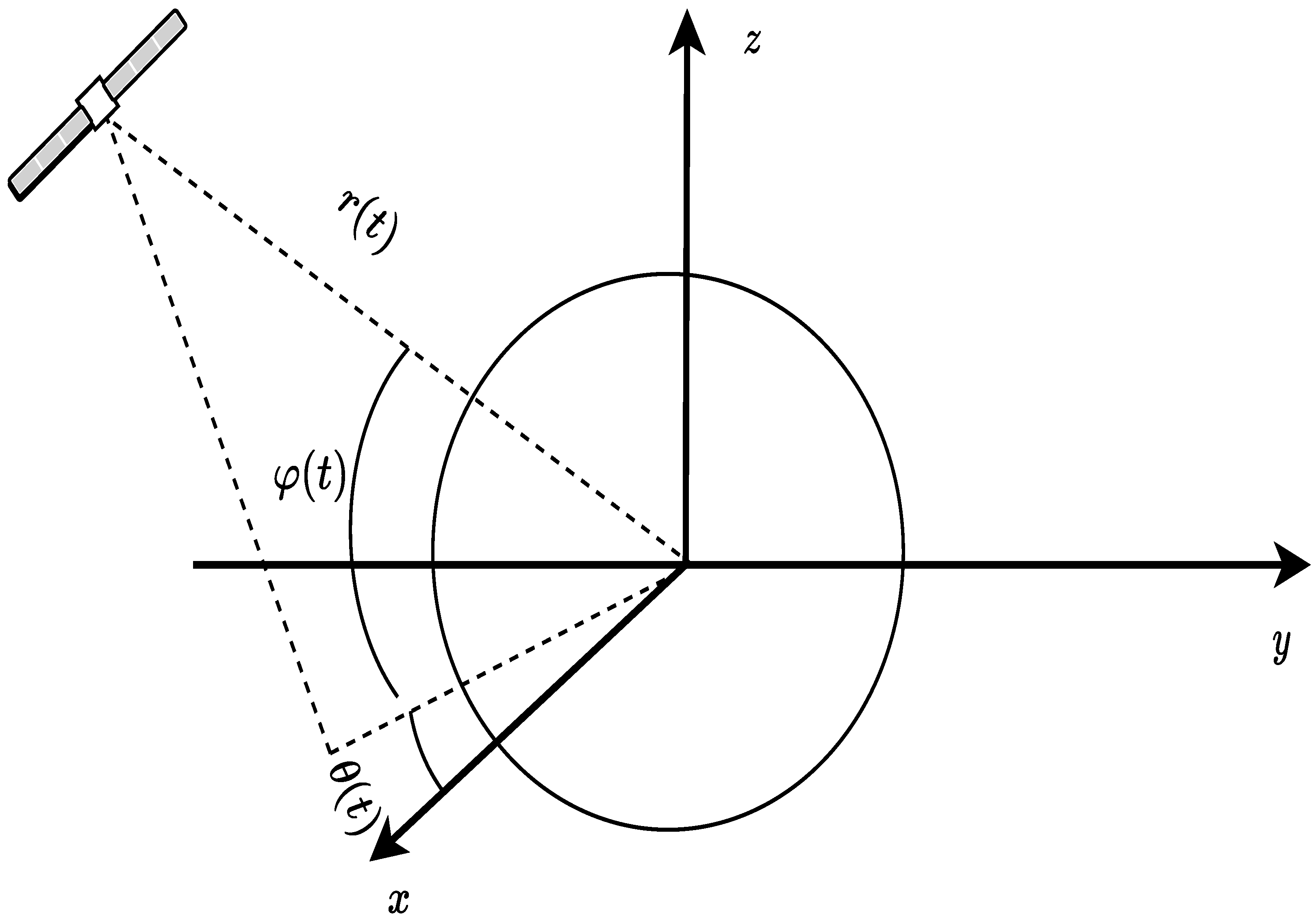
2.1. System Description

In Figure 1, a visually captivating schematic diagram showcases the interplay between Earth and the satellite in space, where the equatorial plane is elegantly represented by the x–y plane, while z symbolizes the polar axis. By skillfully solving the Euler–Lagrange equation, we can gracefully derive the ensuing dynamical equations for our esteemed satellite model [30] as follows:

$$\left\{\begin{array}{c}{\dot{r}}_1=r_2+{\overline{f}}_1(r_1)\hfill \\ {\dot{r}}_2=r_1{\theta }_2^2{cos}^2{\phi }_1+r_1{\phi }_2^2-\frac{c}{r_1^2}+{\overline{f}}_2(r_1,r_2)+\frac{1}{m}{u}_r\hfill \\ {\dot{\theta }}_1={\theta }_2+{\overline{f}}_3(\overline{r},{\theta }_1)\hfill \\ {\dot{\theta }}_2=-2\frac{r_2{\theta }_2}{r_1}+2{\theta }_2{\phi }_2\frac{sin{\phi }_1}{cos{\phi }_1}+{\overline{f}}_4(\overline{r},\overline{\theta })+\frac{1}{m{r}_{1}cos{\phi }_1}{u}_{\theta }\hfill \\ {\dot{\phi }}_1={\phi }_2+{\overline{f}}_5(\overline{r},\overline{\theta },{\phi }_1)\hfill \\ {\dot{\phi }}_2=-{\theta }_2^{2}cos{\phi }_{1}sin{\phi }_1-2\frac{r_2{\theta }_2}{r_1}+{\overline{f}}_6(\overline{r},\overline{\theta },\overline{\phi })+\frac{1}{m{r}_1}{u}_{\phi }\hfill \end{array}\right.$$

(1)

where r, $\theta$, and $\phi$ represent the distance between the satellite and the center of the Earth, the angle traversed by the satellite in the equatorial plane, and the inclination of the satellite on the z-axis, respectively; $c=4\times {10}^{14}$$\mathrm{N}·{\mathrm{m}}^2/\mathrm{kg}$ is a constant related to the universal gravitational constant and the Earth mass; m is the mass of the satellite; the nonlinear function ${\overline{f}}_i(·)$ for $i=1,\dots ,6$ represents the uncertainties present in the satellite orbital control system; and $\overline{r}={[r_1,r_2]}^T,\overline{\theta }={[{\theta }_1,{\theta }_2]}^T,\overline{\phi }={[{\phi }_1,{\phi }_2]}^T$ represent the input variables of the nonlinear functions ${\overline{f}}_i(·)$.

 Remark 1. 

For control schemes employing pole placement, it is imperative to linearize the nonlinear functions of the system in its equilibrium state. Without a loss of generality, let us consider a circular orbit situated on the equator as the satellite’s trajectory. Once in orbit and undisturbed, the satellite can autonomously rotate with an angular velocity ω along a circular path with radius $r_0$. The state equation of the satellite system can be derived as follows:

$$\left\{\begin{array}{c}\dot{x}=Ax+Bu\hfill \\ y=Cx\hfill \end{array}\right.$$

(2)

where $x=[r_1,r_2,{\theta }_1,{\theta }_2,{\phi }_1,{\phi }_2]$, $u=[u_r,u_{\theta },u_{\phi }]$, and y represent the output of the system. The state matrix, input matrix, and output matrix of the system are given by

$$A=\left(\begin{array}{cccccc}0& 1& 0& 0& 0& 0\\ 3{\omega }^2& 0& 0& 2\omega r_0& 0& 0\\ 0& 0& 0& 1& 0& 0\\ 0& -\frac{2\omega }{r_0}& 0& 0& 0& 0\\ 0& 0& 0& 0& 0& 1\\ 0& 0& 0& 0& -{\omega }^2& 0\end{array}\right),B=\left(\begin{array}{ccc}0& 0& 0\\ \frac{1}{m}& 0& 0\\ 0& 0& 0\\ 0& \frac{1}{m{r}_0}& 0\\ 0& 0& 0\\ 0& 0& \frac{1}{m{r}_0}\end{array}\right)$$

(3)

$$C=\left(\begin{array}{cccccc}1& 0& 0& 0& 0& 0\\ 0& 0& 1& 0& 0& 0\\ 0& 0& 0& 0& 1& 0\end{array}\right).$$

(4)

For linear system (2), designing a feedback controller is straightforward. However, satellite modeling involves uncertain nonlinear functions, and we need to perform orbit control in three dimensions. This compels us to consider control schemes tailored for nonlinear systems.

 Assumption 1. 

The reference signals $r_d$, ${\theta }_d$, and ${\phi }_d$ are known and bounded, with their first derivatives also existing.

2.2. Fuzzy Logic Systems

Due to the universal approximation capability of FLSs, they have been widely integrated with adaptive control to address uncertainties in nonlinear systems. The rule base stores fuzzy rules that associate input variables with output variables and consists of the following linguistic rules:

$$\begin{array}{cc}\hfill R^l:& If{x}_{1}is{F}_1^{l}and\dots and{x}_{n}is{F}_n^l\hfill \\ \hfill & Thenyis{B}^l\hfill \end{array}$$

where $x={[x_1,\dots ,x_n]}^T$ and y are the FLS input vector and output vector, respectively. $F_i^l$ and $B^l$ are fuzzy sets connected with the membership functions $u_{F_i^l}(x_i)$ and $u_{B^l}(y)$. In general, the FLS can be represented as follows:

$$y(x)=\frac{{\sum }_{l=1}^N{\overline{y}}_l{\prod }_{i=1}^n{u}_{F_i^l}(x_i)}{{\sum }_{l=1}^N{\prod }_{i=1}^n{u}_{F_i^l}(x_i)}$$

(5)

where the parameter N represents the number of rules and ${\overline{y}}_l=\underset{y\in R}{max}{u}_{B^l}(y)$. From (5), the fuzzy basis function is decomposed into

$${\phi }_l(x)=\frac{{\prod }_{i=1}^n{u}_{F_i^l}(x_i)}{{\sum }_{l=1}^N{\prod }_{i=1}^n{u}_{F_i^l}(x_i)}.$$

(6)

Denote ${\theta }^T=[{\overline{y}}_1,\dots ,{\overline{y}}_n]$ and $\phi (x)={[{\phi }_1(x),\dots ,{\phi }_n(x)]}^T$. The FLS can be expressed as the form of the product between the fuzzy weight vector and the basis function vector:

$$y(x)={\theta }^T\phi (x).$$

(7)

 Lemma 1 

([31]). Assuming $\mathsf{\Theta }(x)$ is a continuous function defined on a compact set Ω, there exists any small constant $ϵ>0$ and an FLS such that

$$\underset{x\in \mathsf{\Omega }}{sup}|\mathsf{\Theta }(x)-{\theta }^T\phi (x)|\le ϵ.$$

(8)

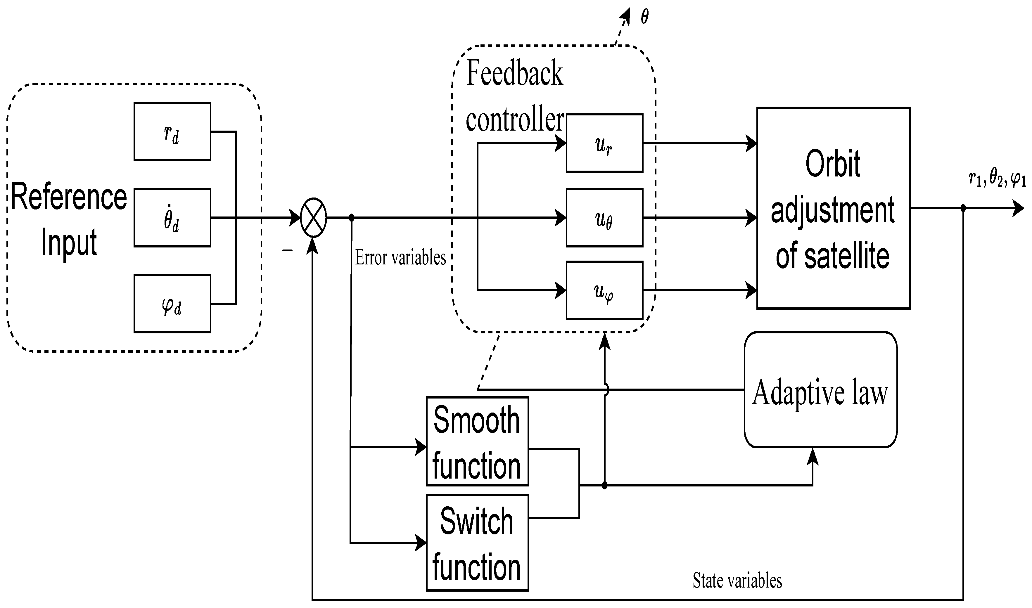
3. Prescribed Adaptive Fuzzy Control Scheme

In this section, we design an adaptive fuzzy control scheme with predetermined performance. A stability analysis is conducted based on the proposed scheme, and the successful establishment of the $L_2$ norm has improved dynamic performance.

3.1. A Class of Smooth Functions

Before proceeding with the controller design, we introduce a class of smooth functions, denoted as

$$s{g}_i(\xi )=\left\{\begin{array}{c}\hfill \begin{array}{cc}\frac{\xi }{\left|\xi \right|},\hfill & \left|\xi \right|\ge {\delta }_i\hfill \\ \frac{\xi }{{({\delta }_i^2-{\xi }^2)}^2+\left|\xi \right|},\hfill & \left|\xi \right|<{\delta }_i\hfill \end{array}\end{array}\right.,i=1,\dots ,6$$

(9)

and a class of switch functions, denoted as

$$f_i(\xi )=\left\{\begin{array}{cc}1,\hfill & \left|\xi \right|\ge {\delta }_i\hfill \\ 0,\hfill & \left|\xi \right|<{\delta }_i\hfill \end{array}\right.,i=1,\dots ,6$$

(10)

are introduced to facilitate the controller design. For clarity, the notations ${\delta }_i,i=1,\dots ,6$ are positive constants and $\xi$ represents the error between the state variable and the reference signal.

3.2. Feedback Controller Design

For the radial subsystem, the error variables are defined as follows:

$$\left\{\begin{array}{c}{\xi }_{r_1}=r_1-r_d\hfill \\ {\xi }_{r_2}=r_2-{\alpha }_{r_1}^{*}\hfill \end{array}\right.$$

(11)

where $r_d$ is the satellite trajectory tracking reference signal, and ${\alpha }_{r_1}^{*}$ will be provided in the subsequent design of the virtual controller.

The radial controller design:

The derivative of ${\xi }_{r1}$ is

$$\begin{array}{c}\hfill {\dot{\xi }}_{r_1}={\dot{r}}_1-{\dot{r}}_d={\xi }_{r_2}+{\alpha }_{r_1}^{*}+{\overline{f}}_1(r_1)-{\dot{y}}_r={\xi }_{r_2}+{\alpha }_{r_1}^{*}+{\Delta }_1-{\delta }_{2}s{g}_1\end{array}$$

(12)

where ${\Delta }_1$ is a function related to the fuzzy logic system and its approximation error, defined as

$${\Delta }_1={\overline{f}}_1(r_1)+{\delta }_{2}s{g}_1({\xi }_1)+{\dot{r}}_d={\theta }_1^{*T}{\varphi }_1+d_1={\theta }_0^{*}{\psi }_1$$

(13)

where ${\theta }_0^{*}$ is relevant to the fuzzy weight vector and the fuzzy logic systems error. The adaptive parameter ${\theta }_0^{*}$ is expressed as

$${\theta }_0^{*}=[{\theta }_1^{*T},\dots ,{\theta }_6^{*T},d_1,\dots ,d_6].$$

(14)

We use ${\theta }_i^{*}$ to represent the fuzzy weight vector, such as ${\overline{y}}_l$ in (5); $d_i$ to represent the error constant, such as $ϵ$ in (8); and ${\omega }_i,i=1,\dots ,6$ to represent the vector related to the basis functions as follows:

$${\psi }_1={[{\varphi }_1,\underset{5}{\underbrace{0,\dots ,0}},1,\underset{5}{\underbrace{0,\dots ,0}}]}^T,$$

(15)

$${\psi }_i={[\underset{i-1}{\underbrace{0,\dots ,0}},{\varphi }_i,\underset{6-i}{\underbrace{0,\dots ,0}},\underset{i-1}{\underbrace{0,\dots ,0}},1,\underset{6-i}{\underbrace{0,\dots ,0}}]}^T$$

(16)

where ${\varphi }_i$ denotes the fuzzy basis function similar to $\phi$ in (6). Then, one can obtain that

$${\theta }^{*}=\left|\right|{\theta }_0^{*}{\left|\right|}_{\infty }=\underset{t\ge 0}{sup}\left|\right|{\theta }_0^{*}(t)\left|\right|$$

(17)

We denote ${\omega }_i=s{g}_i({\xi }_i)\sqrt{{\psi }_i^T{\psi }_i}$.

We combine the unknown weight vector ${\theta }_i^{*T}$ and the approximation error $d_i$ into an unknown vector function ${\theta }^{*}$, and ${\theta }^{*}$ is bounded. Unlike traditional fuzzy logic systems that ignore approximation errors, we further consider the handling of errors. The boundedness of ${\theta }^{*}$ is guaranteed, and this property is related to the calculation of the convergence time.

The Lyapunov function is chosen as

$$V_{1,1}=\frac{1}{2}(|{\xi }_{r_1}{|-{\delta }_1)}^2{f}_1,$$

(18)

and its derivative is

$${\dot{V}}_{1,1}=(|{\xi }_{r_1}|-{\delta }_1)f_{1}s{g}_1({\xi }_{r_1})({\xi }_{r_2}+{\alpha }_{r_1}^{*}+{\theta }^{*}{\mathrm{\Psi }}_1).$$

(19)

The virtual controller ${\alpha }_{r_1}^{*}$ is chosen as

$${\alpha }_{r_1}^{*}=-c_1(|{\xi }_{r_1}|-{\delta }_1)s{g}_1({\xi }_{r_1})-\theta {\omega }_1$$

(20)

Substituting (20) into (19), we have

$$\begin{array}{cc}\hfill {\dot{V}}_{1,1}\le & -c_1(|{\xi }_{r_1}|-{\delta }_1{)}^2{f}_1+({\xi }_{r_1}|-{\delta }_1)f_1(|{\xi }_{r_2}|-{\delta }_2)f_{2}s{g}_2^2+\tilde{\theta }{\tau }_1\hfill \end{array}$$

(21)

for ${\tau }_1=(|{\xi }_{r_1}|-{\delta }_1)f_{1}s{g}_1{\omega }_1$.

 Remark 2. 

Traditional backstepping control schemes involve directly solving derivatives of the virtual controller. As the system order increases, the computational complexity also increases. Dynamic surface control and command filtering control address this issue by designing filters to replace the derivatives of the virtual controller. While these methods resolve the issue of complexity, the design of filters can be complex, and they also introduce the challenge of error compensation. In our approach, we successfully address the problem of exploding complexity by using a fuzzy logic system combined with smooth functions.

For the second step of backstepping control design, we design the radial control law using the following Lyapunov function:

$$V_{1,2}=\frac{1}{2}(|{\xi }_{r_2}{|-{\delta }_2)}^2{f}_2+V_{1,1}$$

(22)

and the derivative is computed as

$$\begin{array}{cc}\hfill {\dot{V}}_{1,2}=& (|{\xi }_{r_2}|-{\delta }_2)f_{2}s{g}_2{\dot{\xi }}_{r_2}+{\dot{V}}_{1,1}\hfill \\ \hfill \le & (|{\xi }_{r_2}|-{\delta }_2)f_{2}s{g}_2(r_1{\theta }_2^2{cos}^2{\phi }_1+r_1{\phi }_2^2+{\Delta }_2+\frac{1}{m}\sum _{i=1}^p{u}_{r_i})\hfill \\ \hfill & -c_1(|{\xi }_{r_1}|-{\delta }_1)f_1-k_1(|{\xi }_{r_1}{|-{\delta }_1)}^4{f}_1+\tilde{\theta }{\tau }_1\hfill \\ \hfill & +(|{\xi }_{r_2}|-{\delta }_2)f_{2}s{g}_2\frac{\partial {\alpha }_{r_1}^{*}}{\theta }(\gamma {\tau }_2-\dot{\theta })\hfill \end{array}$$

(23)

where the composite function is defined as

$$\begin{array}{cc}\hfill {\Delta }_2=& s{g}_2(|{\xi }_{r_1}|-{\delta }_1)f_1-\frac{c}{r_1^2}+{\overline{f}}_{r_2}(r_1,r_2)-\frac{\partial {\alpha }_{r_1}^{*}}{\partial r_1}{\dot{r}}_1-\frac{\partial {\alpha }_{r_1}^{*}}{\partial y_r}{\dot{y}}_r-\frac{\partial {\alpha }_{r_1}^{*}}{\partial \theta }\gamma {\tau }_2\hfill \\ \hfill =& {\theta }_2^{*T}{\varphi }_2+d_2={\theta }_0^{*}{\mathrm{\Psi }}_2.\hfill \end{array}$$

(24)

The function ${\Delta }_2$ is approximated using a fuzzy logic system, addressing not only the uncertainty in system modeling but also ensuring that the designed controller is nonsingular.

We choose the controller $u_r$ as

$$\begin{array}{cc}\hfill u_r=& -m{c}_2(|{\xi }_{r2}|-{\delta }_2)s{g}_2-\theta {\omega }_2.\hfill \end{array}$$

(25)

Substituting $u_r$ into (23), we have

$$\begin{array}{cc}\hfill {\dot{V}}_{1,2}\le & -\sum _{i=1}^2{c}_i(|{\xi }_{r_i}|-{\delta }_i{)}^2{f}_i+\tilde{\theta }{\tau }_2+(|{\xi }_{r_2}|-{\delta }_2)f_{2}s{g}_2\frac{\partial {\alpha }_{r_1}^{*}}{\partial \theta }(\gamma {\tau }_2-\dot{\theta })\hfill \end{array}$$

(26)

for ${\tau }_2=(|{\xi }_{r2}-{\delta }_2|)f_{2}s{g}_2{\omega }_2+{\tau }_1$.

The tangential controller design:

For the tangential subsystem, the error variable is defined as

$$\left\{\begin{array}{c}{\xi }_{{\theta }_1}={\theta }_1-{\theta }_d\hfill \\ {\xi }_{{\theta }_2}={\theta }_2-{\alpha }_{{\theta }_1}^{*},\hfill \end{array}\right.$$

(27)

where ${\theta }_d$ represents the angular velocity of Earth’s rotation.

The virtual controller ${\alpha }_{{\theta }_1}^{*}$ is designed as

$${\alpha }_{{\theta }_1}^{*}=-c_3(|{\xi }_{{\theta }_1}|-{\delta }_3)s{g}_3({\xi }_{{\theta }_1})-\theta {\omega }_3.$$

(28)

The Lyapunov candidate function of the subsystems is considered

$$V_{2,1}=V_{1,2}+\frac{1}{2}(|{\xi }_{{\theta }_1}{|-{\delta }_3)}^2{f}_3$$

(29)

We consider a complex composite function

$$\begin{array}{cc}\hfill {\Delta }_3=& -{\delta }_{4}sg3+{\overline{f}}_3(\overline{r},{\theta }_1)+{\dot{\theta }}_d-\frac{\partial {\alpha }_{r_1}^{*}}{\partial \theta }(|{\xi }_{r_2}|-{\delta }_2)f_{2}s{g}_2\gamma {\omega }_3\hfill \\ \hfill =& {\theta }_3^{*T}{\varphi }_3+d_3={\theta }_0^{*}{\mathrm{\Psi }}_3\hfill \end{array}$$

(30)

By using (28) and (30), we can compute ${\dot{V}}_{2,1}$ as follows:

$$\begin{array}{cc}\hfill {\dot{V}}_{2,1}\le & -\sum _{i=1}^2{c}_i(|{\xi }_{r_i}|-{\delta }_i{)}^2{f}_i+\tilde{\theta }{\tau }_3-c_3(|{\xi }_{{\theta }_1}{|-{\delta }_3)}^2{f}_3\hfill \\ \hfill & +(|{\xi }_{{\theta }_2}|-{\delta }_4)f_{4}s{g}_4^2(|{\xi }_{{\theta }_1}|-{\delta }_3)f_3\hfill \\ \hfill & +(|{\xi }_{r_2}|-{\delta }_2)f_{2}s{g}_2\frac{\partial {\alpha }_{r_1}^{*}}{\partial \theta }(\gamma {\tau }_3-\dot{\theta })\hfill \end{array}$$

(31)

for ${\tau }_3=(|{\xi }_{{\theta }_1}|-{\delta }_3)f_{3}s{g}_3{\omega }_3+{\tau }_2$.

The controller $u_{\theta }$ is designed as

$$u_{\theta }=-c_4(|{\xi }_{{\theta }_2}|-\delta 4)s{g}_4-\theta {\omega }_4.$$

(32)

We design a composite function as

$$\begin{array}{cc}\hfill {\Delta }_4=& s{g}_4(|{\xi }_{{\theta }_1}|-{\delta }_3)f_3-2\frac{r_2{\theta }_2}{r_1}+2{\theta }_2{\phi }_2\frac{sin{\phi }_1}{cos{\phi }_1}-\frac{\partial {\alpha }_{{\theta }_1}^{*}}{{\theta }_1}({\theta }_2+{\overline{f}}_3(\overline{r},{\theta }_1))\hfill \\ \hfill & +{\overline{f}}_4(\overline{r},\overline{\theta })+(|{\xi }_{r_2}|-{\delta }_2)f_{2}s{g}_2\frac{\partial {\alpha }_{r_1}^{*}}{\theta }\gamma {\omega }_4-\frac{\partial {\alpha }_{{\theta }_1}^{*}}{\theta }\gamma {\tau }_4\hfill \\ \hfill =& {\theta }_4^{*T}{\varphi }_4+d_4={\theta }_0^{*}{\mathrm{\Psi }}_4.\hfill \end{array}$$

(33)

We consider the following Lyapunov function candidate:

$$V_{2,2}=V_{2,1}+\frac{1}{2}(|{\xi }_{{\theta }_2}{|-{\delta }_4)}^2{f}_4$$

(34)

whose derivative is computed as

$$\begin{array}{cc}\hfill {\dot{V}}_{2,2}\le & -\sum _{i=1}^2{c}_i(|{\xi }_{r_i}|-{\delta }_i{)}^2{f}_i+\tilde{\theta }{\tau }_4-\sum _{i=3}^4{c}_i(|{\xi }_{{\theta }_i}{|-{\delta }_i)}^2{f}_i\hfill \\ \hfill & +(|{\xi }_{r_2}|-{\delta }_2)f_{2}s{g}_2\frac{\partial {\alpha }_{r_1}^{*}}{\partial \theta }(\gamma {\tau }_4-\dot{\theta })\hfill \\ \hfill & +(|{\xi }_{{\theta }_2}|-{\delta }_4)f_{4}s{g}_4\frac{\partial {\alpha }_{{\theta }_1}^{*}}{\partial \theta }(\gamma {\tau }_4-\dot{\theta })\hfill \end{array}$$

(35)

for ${\tau }_4=(|{\xi }_{{\theta }_2}|-{\delta }_4)f_{4}s{g}_4{\omega }_4+{\tau }_3$.

The tilted direction controller design:

For the tilted system relative to the equatorial plane, the error variable is defined as

$$\left\{\begin{array}{c}{\xi }_{{\phi }_1}={\phi }_1-{\phi }_d\hfill \\ {\xi }_{{\phi }_2}={\phi }_2-{\alpha }_{{\phi }_1}^{*}.\hfill \end{array}\right.$$

(36)

The virtual controller is designed as

$${\alpha }_{{\phi }_1}^{*}=-c_5(|{\xi }_{{\phi }_1}|-{\delta }_5)s{g}_5-\theta {\omega }_5$$

(37)

The Lyapunov candidate function of the subsystems is considered

$$V_{3,1}=V_{2,2}+\frac{1}{2}(|{\xi }_{{\phi }_1}{|-{\delta }_5)}^2{f}_5.$$

(38)

We consider a complex composite function

$$\begin{array}{cc}\hfill {\Delta }_5=& -{\delta }_{6}s{g}_5+{\overline{f}}_5(\overline{r},\overline{\theta },{\phi }_1)-(|{\xi }_{r_2}|-{\delta }_2)f_{2}s{g}_2\frac{\partial {\alpha }_{r_1}^{*}}{\theta }\gamma {\omega }_5\hfill \\ \hfill & -(|{\xi }_{{\theta }_2}|-{\delta }_4)f_{4}s{g}_4\frac{\partial {\alpha }_{{\theta }_1}^{*}}{\theta }\gamma {\omega }_5\hfill \\ \hfill =& {\theta }_5^{*T}{\varphi }_5+d_5={\theta }_0^{*}{\mathrm{\Psi }}_5.\hfill \end{array}$$

(39)

The derivate of (38) is calculated as

$$\begin{array}{cc}\hfill {\dot{V}}_{3,1}\le & -\sum _{i=1}^2{c}_i(|{\xi }_{r_i}|-{\delta }_i{)}^2{f}_i+\tilde{\theta }{\tau }_5-\sum _{i=3}^4{c}_i(|{\xi }_{{\theta }_i}{|-{\delta }_i)}^2{f}_i\hfill \\ \hfill & -c_5(|{\xi }_{{\phi }_1}|-{\delta }_5{)}^2{f}_5+(|{\xi }_{r_2}|-{\delta }_2)f_{2}s{g}_2\frac{\partial {\alpha }_{r_1}^{*}}{\partial \theta }(\gamma {\tau }_5-\dot{\theta })\hfill \\ \hfill & +(|{\xi }_{{\theta }_2}|-{\delta }_4)f_{4}s{g}_4\frac{\partial {\alpha }_{{\theta }_1}^{*}}{\partial \theta }(\gamma {\tau }_5-\dot{\theta })\hfill \\ \hfill & +(|{\xi }_{{\phi }_2}|-{\delta }_6)f_{6}s{g}_6^2(|{\xi }_{{\phi }_1}|-{\delta }_5)f_5\hfill \end{array}$$

(40)

for ${\tau }_5=(|{\xi }_{{\phi }_1}|-{\delta }_5)f_{5}s{g}_5{\omega }_5+{\tau }_4$.

Controller $u_{\phi }$ is designed as

$$u_{\phi }=-c_6(|{\xi }_{{\phi }_2}|-{\delta }_6)s{g}_6-\theta {\omega }_6.$$

(41)

We design the composite function as

$$\begin{array}{cc}\hfill {\Delta }_6=& s{g}_6(|{\xi }_{{\phi }_1}|-{\delta }_5)f_5-{\theta }_2^{2}cos{\phi }_{1}sin{\phi }_1-2\frac{r_2{\theta }_2}{r_1}+{\overline{f}}_6(\overline{r},\overline{\theta },\overline{\phi })\hfill \\ \hfill & -\frac{\partial {\alpha }_{{\phi }_1}^{*}}{\partial {\phi }_1}({\phi }_2+{\overline{f}}_5(\overline{r},\overline{\theta },{\phi }_1))-\frac{\partial {\alpha }_{{\phi }_1}^{*}}{\partial \theta }\gamma {\tau }_6-(|{\xi }_{r_2}|-{\delta }_2)f_{2}s{g}_2\frac{\partial {\alpha }_{r_1}^{*}}{\theta }\gamma {\omega }_6\hfill \\ \hfill =& {\theta }_6^{*T}{\varphi }_6+d_6={\theta }_0^{*}{\mathrm{\Psi }}_6.\hfill \end{array}$$

(42)

We consider the following Lyapunov candidate function:

$$V=V_{3,1}+\frac{1}{2}(|{\xi }_{{\phi }_2}{|-{\delta }_6)}^2{f}_6+\frac{1}{2\gamma }{\tilde{\theta }}^2$$

(43)

and compute its derivative

$$\begin{array}{cc}\hfill \dot{V}\le & -\sum _{i=1}^2{c}_i(|{\xi }_{r_i}|-{\delta }_i{)}^2{f}_i-\sum _{i=3}^4{c}_i(|{\xi }_{{\theta }_{i-2}}|-{\delta }_i{)}^2{f}_i-\sum _{i=5}^6{c}_i(|{\xi }_{{\phi }_{i-4}}{|-{\delta }_i)}^2{f}_i\hfill \\ \hfill & +(|{\xi }_{r_2}|-{\delta }_2)f_{2}s{g}_2\frac{\partial {\alpha }_{r_1}^{*}}{\partial \theta }(\gamma {\tau }_6-\dot{\theta })+(|{\xi }_{{\theta }_2}|-{\delta }_4)f_{4}s{g}_4\frac{\partial {\alpha }_{{\theta }_1}^{*}}{\partial \theta }(\gamma {\tau }_6-\dot{\theta })\hfill \\ \hfill & +(|{\xi }_{{\phi }_2}|-{\delta }_6)f_{6}s{g}_6\frac{\partial {\alpha }_{{\phi }_1}^{*}}{\theta }(\gamma {\tau }_6-\dot{\theta })+\tilde{\theta }{\tau }_6-\frac{1}{\gamma }\tilde{\theta }\dot{\theta }.\hfill \end{array}$$

(44)

To ensure that the selected Lyapunov derivative remains non-increasing, the adaptive laws related to the fuzzy logic system are chosen as

$$\dot{\theta }=\gamma {\tau }_6.$$

(45)

Figure 2 illustrates a block diagram of our designed adaptive fuzzy control method with prescribed accuracy. The diagram, focusing on the flow of system signals, presents a control scheme for a multiple-input–multiple-output (MIMO) system. Specifically emphasized are the smooth functions, switch functions, and adaptive law, with the fuzzy logic system omitted for clarity.

3.3. Stability Analysis

In this section, the primary focus is to establish the boundedness of closed-loop signals and the convergence performance of errors for a satellite system. Additionally, the dynamic behavior of errors in terms of performance is analyzed.

 Theorem 1. 

We consider the satellite orbit control system described by (1) and assume Assumption 1 is satisfied. If the virtual controllers specified by (20), (28), and (37); the feedback controllers defined by (25), (32), and (41); and the adaptive laws given by (45) are selected, then the following results can be drawn that all closed-loop signal are bounded, and the position tracking error ${\xi }_1$ can converge to a predetermined interval $[-{\delta }_1,{\delta }_1]$.

Proof of Theorem 1. 

We can consider the following candidate Lyapunov function:

$$V(t)=\frac{1}{2}{\xi }^T\xi +\frac{1}{2\gamma }{\tilde{\theta }}^2,$$

(46)

where $\xi =[(|{\xi }_{r_1}|-{\delta }_1)f_1,\dots ,(|{\xi }_{{\phi }_2}|-{\delta }_6{)f_6]}^T$. Substituting (45) into (44), the simplified derivative of the Lyapunov function can be obtained as follows:

$$\begin{array}{cc}\hfill \dot{V}(t)\le & -\sum _{i=1}^2{c}_i(|{\xi }_{r_i}|-{\delta }_i{)}^2{f}_i-\sum _{i=3}^4{c}_i(|{\xi }_{{\theta }_{i-2}}{|-{\delta }_i)}^2{f}_i\hfill \\ \hfill & -\sum _{i=5}^6{c}_i(|{\xi }_{{\phi }_{i-4}}{|-{\delta }_i)}^2{f}_i.\hfill \\ \hfill \end{array}$$

(47)

Therefore, the selected Lyapunov function is non-increasing. Clearly, we have $V(t)\le V(0)$. In other words, the boundedness of $\xi$ and $\tilde{\theta }$ depends on whether $V(0)$ is bounded. Therefore, the boundedness of $\xi$ and $\tilde{\theta }$ is ensured for $t\in [0,+\infty ]$. Since ${\xi }_{r_1}$ and $y_r$ belong to $L^{\infty }$, we can conclude that $r_1$ also belongs to $L^{\infty }$. Furthermore, as the virtual controller ${\alpha }_1$ is a function of ${\xi }_{r_1}$, $\tilde{\theta }$, and $r_2={\xi }_{r_2}+{\alpha }_1$, the boundedness of $r_2$ is also ensured. Similarly, the boundedness of other state variables in the satellite control system, such as ${\theta }_1$, ${\theta }_2$, ${\phi }_1$, and ${\phi }_2$, is also guaranteed. Thus, the boundedness of all closed-loop signals is established. Combining the properties of the selected Lyapunov function and Barbalat’s Lemma, we can conclude that ${lim}_{t\to \infty }\dot{V}(t)=0$. Therefore, as $t\to \infty$, ${\xi }_{r_1}\in [-{\delta }_1,{\delta }_1]$, ${\xi }_{{\theta }_1}\in [-{\delta }_3,{\delta }_3]$, ${\xi }_{{\phi }_1}\in [-{\delta }_5,{\delta }_5]$, which means that the defined error can converge within our predetermined error bounds. □

 Theorem 2. 

The bound of the L2 norm of the position error system is introduced, which is expressed as follows:

$$\left|\right|(|{\xi }_{r_1}|-{\delta }_1)f_1{\left|\right|}_2\le \frac{1}{\sqrt{c_1}}{\left[\frac{1}{2\gamma }{\tilde{\theta }}^2(0)\right]}^{\frac{1}{2}}.$$

(48)

Proof of Theorem 2. 

From (43), we have

$$V(0)=\sum _{i=1}^6\frac{1}{2}(|\overline{\xi }\left[i\right](0){|-{\delta }_i)}^2{f}_i+\frac{1}{2\gamma }{\tilde{\theta }}^2(0),$$

(49)

where $\overline{\xi }=[{\xi }_{r_1},{\xi }_{r_2},{\xi }_{{\theta }_1},{\xi }_{{\theta }_2},{\xi }_{{\phi }_1},{\xi }_{{\phi }_2}]$. By using the initialization conditions from [29], we can ensure that $\left|\xi \left[i\right]\right|\le {\delta }_i$, $i=1,\dots ,6$, which leads to ${\sum }_{i=1}^6(|\xi \left[i\right]|-{\delta }_i{)}^2{f}_i=0$. Then, we obtain the result in (48). □

 Remark 3. 

By establishing the L2 norm, we can adjust the controller parameters to improve the system’s dynamic performance. It is worth noting that we employed initial value conditions, ensuring that adjusting the controller parameters did not affect the error function at each step.

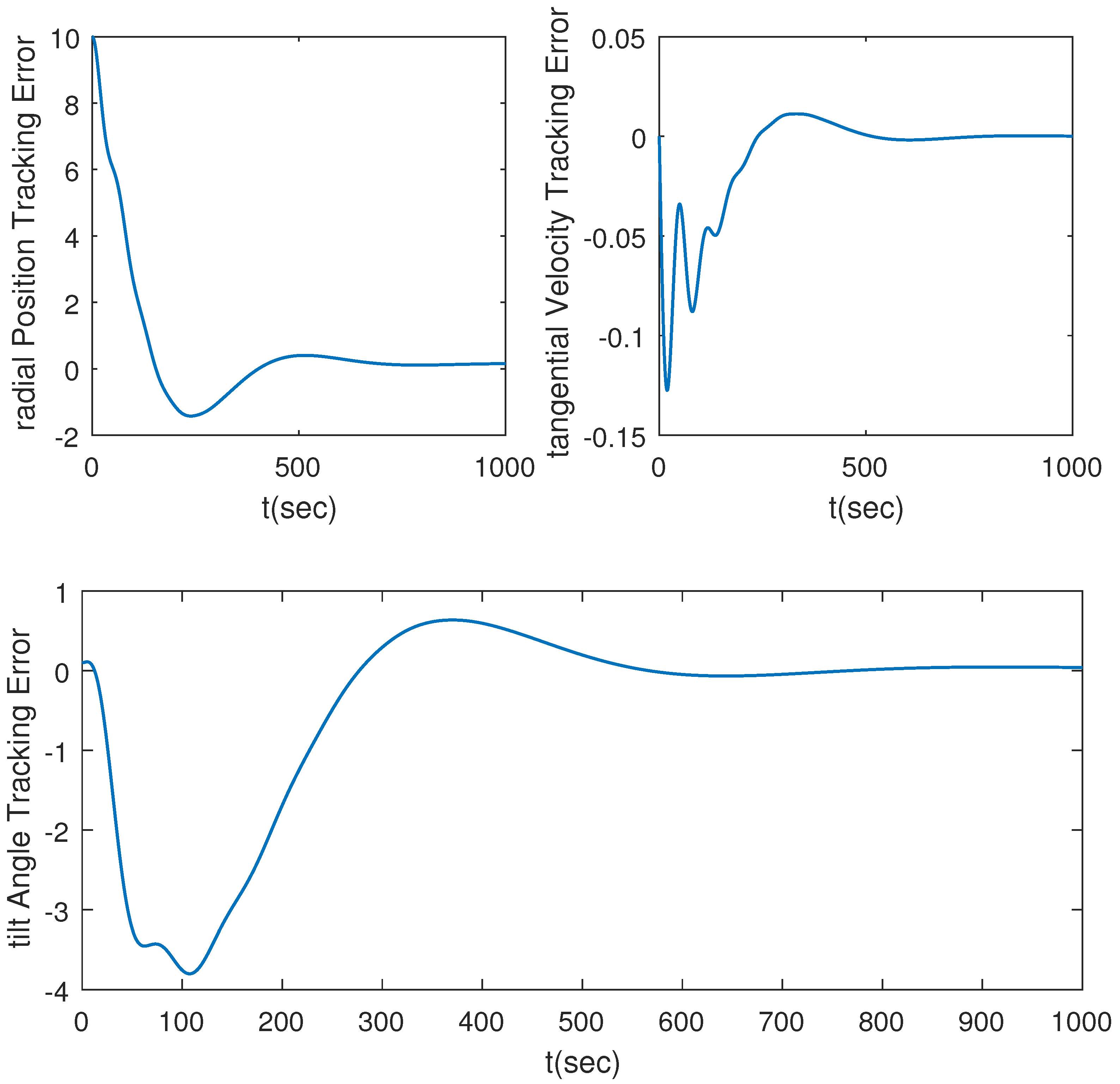
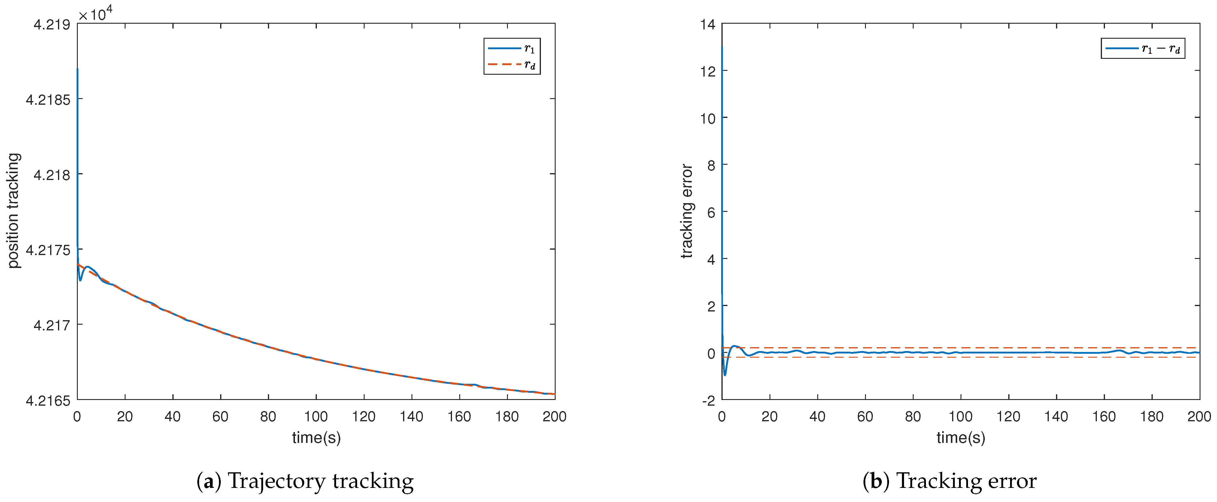
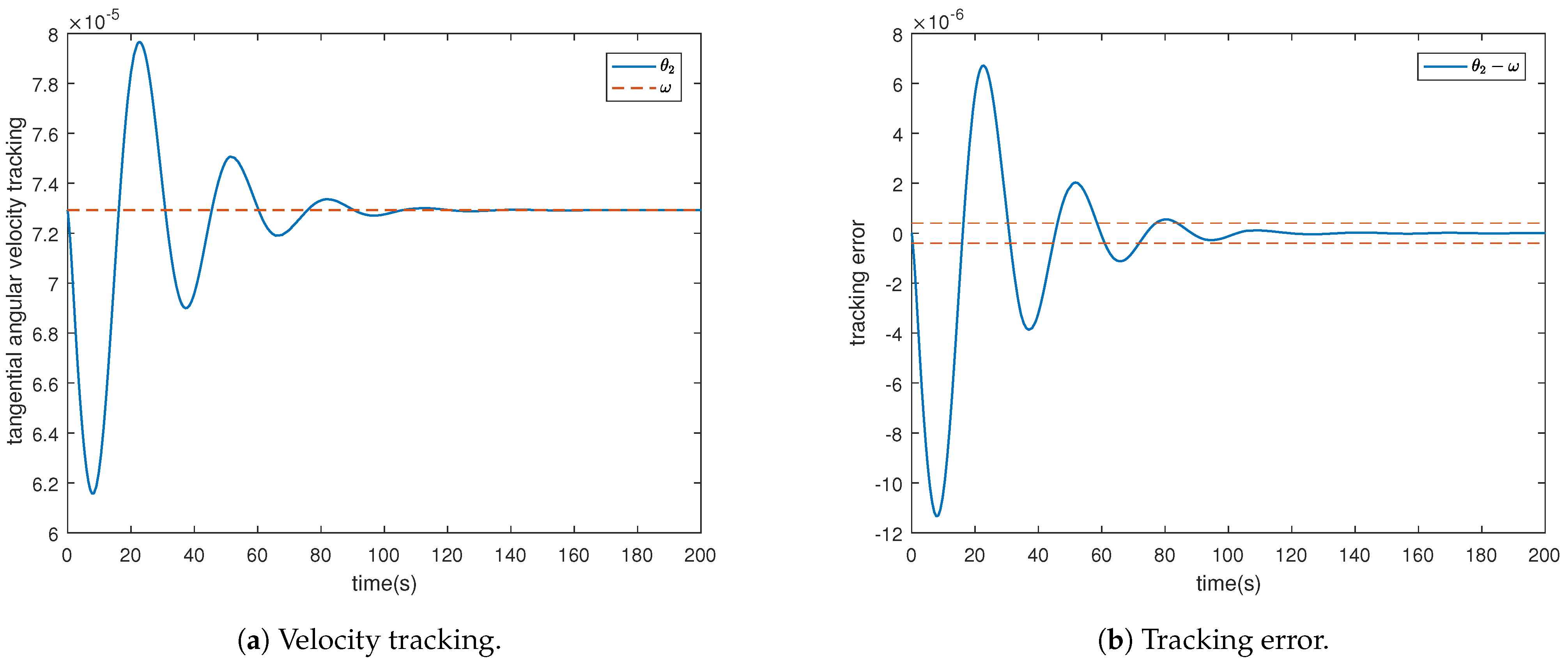
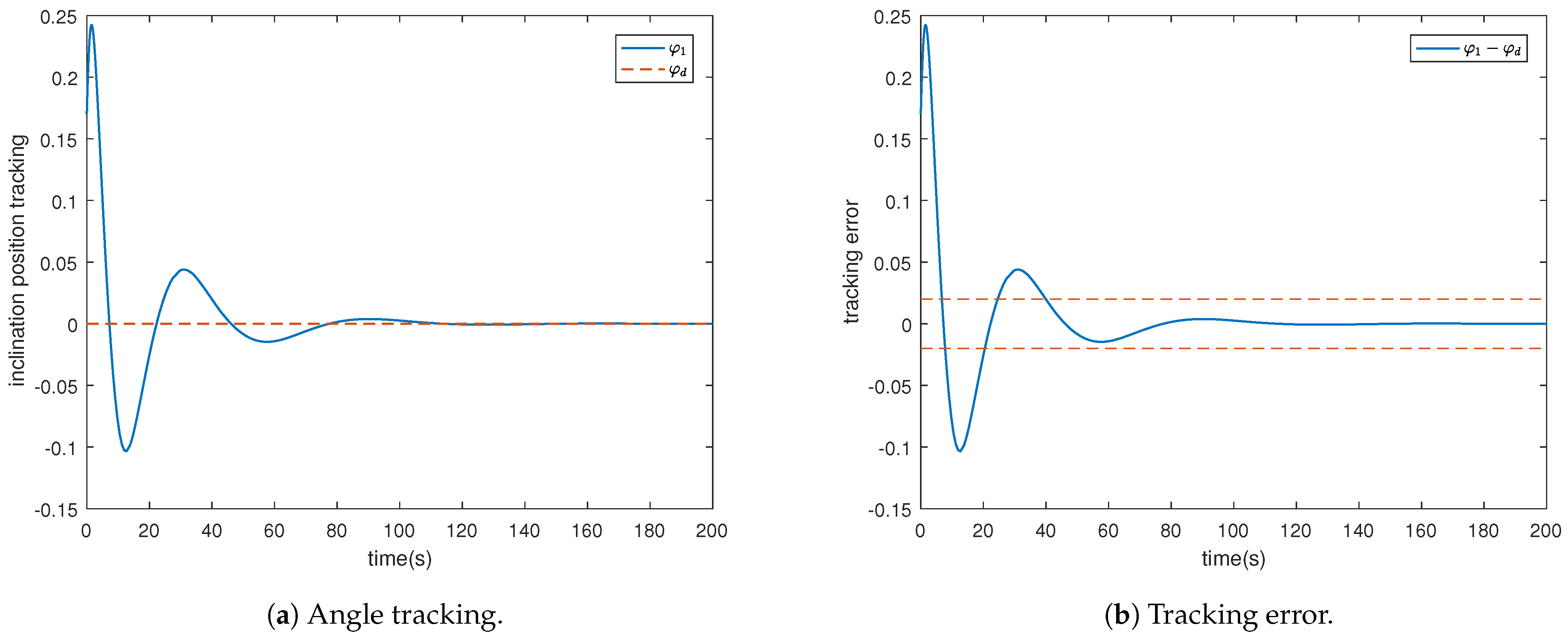
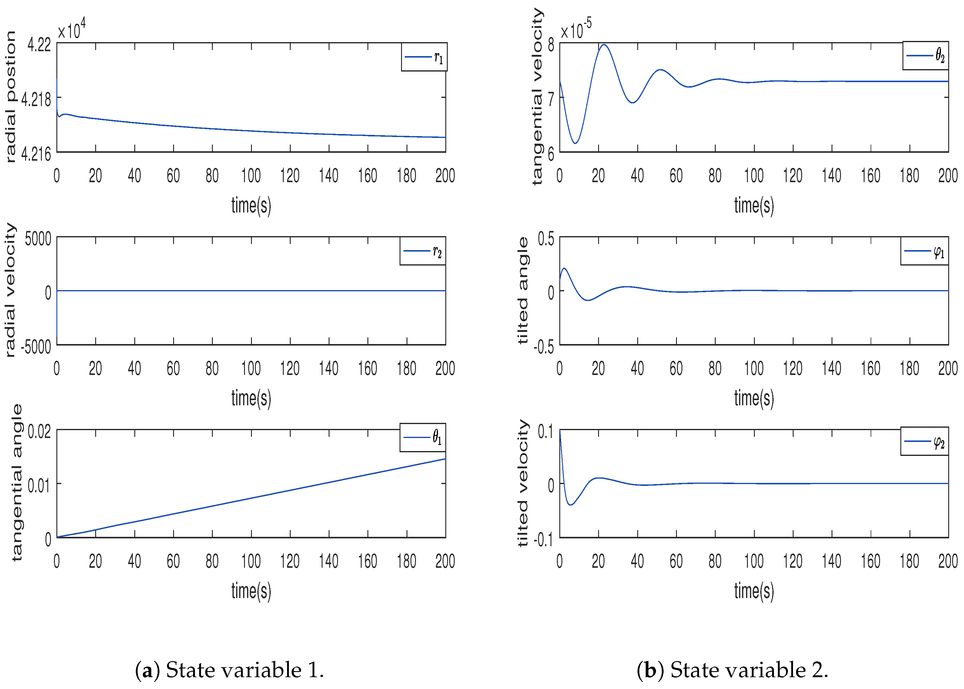
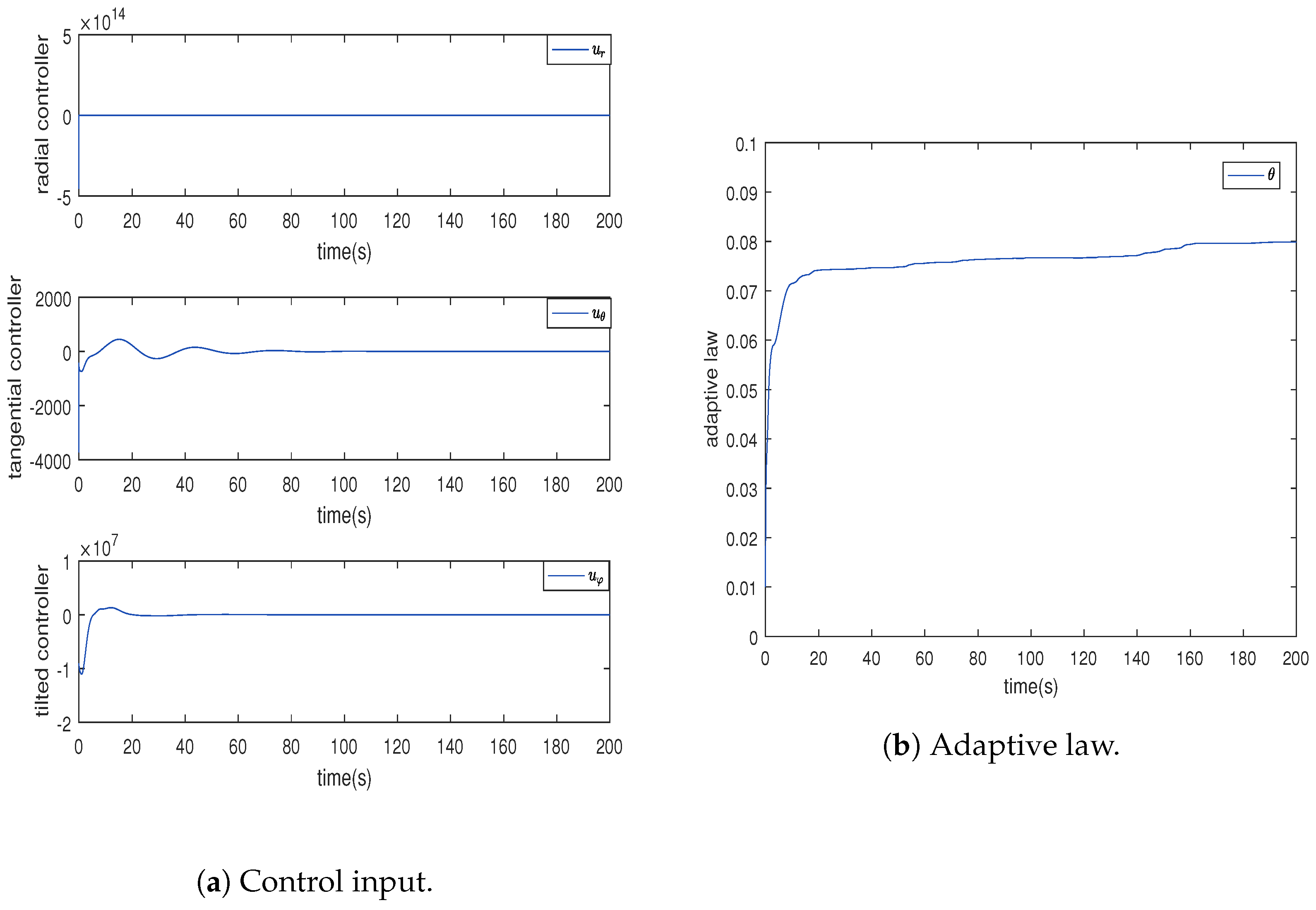
4. Simulation Results

This section verifies the effectiveness of the fault-tolerant control scheme designed above by considering the Geostationary Earth Orbit Satellite. The reference signal $r_d$ was set as $r_d$ = 42,164 + $10e^{-0.01t}$. The angular velocity of the Earth rotation was set to ${\theta }_d=7.2921150\times {10}^{-5}·t$. We set the satellite orbit to be equatorial; hence, ${\phi }_d=0$. The mass of the GEOS is m = 5400 kg [32].

The controller design parameters and corresponding initial values were set as follows: ${\delta }_1=0.01,{\delta }_2=1,{\delta }_3=0.88,{\delta }_4=1,{\delta }_5=1,{\delta }_6=1,c_1=0.01,c_2=1,c_3=1,c_4=1,c_5=1,c_6=1$. The initial values of the state variables were set to 42,187; 0; 0; 7.2921150 ×${10}^{-5}$; 0.1; and 0.1. Additionally, the initial value of the adaptive law was set as $\theta (0)=0.01$;

Simulation Results: The simulation results are shown in Figure 3, Figure 4, Figure 5, Figure 6, Figure 7 and Figure 8. The result of the linear control scheme for the satellite orbit adjustment system is shown in Figure 3. The satellite orbit adjustment model was linearized around the equilibrium point to obtain the linear model, as in Equation (2). Using the pole placement control scheme, we determined the closed-loop system poles based on the specified performance criteria: rise time $t_s=300$ s, damping ratio $\xi =0.5$, and undamped natural frequency ${\omega }_n=0.267$. The resulting poles were set as $p_{0r}=-0.04\pm 0.1i$ and $p_{0\theta }$ and $p_{0\phi }=-0.0133\pm 0.023i$, from which the state feedback parameters were derived. The experimental results, as shown in Figure 1, indicate that the obtained results can only guarantee the convergence of the state error to the vicinity of 0. Additionally, the controller designed using direct pole placement cannot be directly applied to nonlinear systems.

Figure 4 illustrates that the satellite orbit adjustment in the radial direction relative to Earth can operate within the prescribed range of $[-0.01,0.01]$. In Figure 5 and Figure 6, the satellite’s angular velocity tracks Earth’s rotational speed $\omega$, with the satellite inclination angle set to $0^{\circ }$, meaning it is in the equatorial plane. Additionally, their tracking errors are within the predetermined range. It can be observed from Figure 7 and Figure 8 that the control scheme we designed ensures that system state variables, control inputs, and adaptive laws are all bounded.

The tracking errors shown in Figure 4, Figure 5 and Figure 6 demonstrate the effectiveness of our designed control scheme in ensuring convergence of the defined error variables within a specified range. However, for certain control schemes employing fuzzy logic systems to handle uncertainties, it cannot be guaranteed that the derivative of the defined Lyapunov function is negative semi-definite, resulting in $\dot{V}\le -cV+D$, where c and D are positive integers. Consequently, this implies that the convergence error of the system is confined to a small vicinity around 0. Therefore, proper parameter tuning becomes essential for achieving satisfactory performance.

The various state variables, control inputs, and adaptive law of the satellite system are shown in Figure 7 and Figure 8, indicating that their boundedness is guaranteed. As we are considering the regulation of real satellite orbits, the control inputs to the system may be relatively large.

As for the graph of ${\theta }_1$, since ${\theta }_1$ represents the accumulation of the angle traveled by the satellite around the Earth, it is a rising straight line with a slope of the rotation rate $\omega$ after the satellite completes one revolution, the angle accumulation is reset to zero, and the accumulation restarts. That is, the graph of ${\theta }_1$ is similar to a sawtooth wave.

5. Conclusions

A precision control scheme based on adaptive fuzzy technology is proposed for satellite orbit adjustment. This control scheme offers several advantages over existing methods. Firstly, it effectively avoids the “singularity obstacle” problem that can occur during orbit adjustment, ensuring smooth and stable operation of the satellite. Additionally, it takes into account the approximation error of the fuzzy logic system, enhancing the accuracy and reliability of the control scheme.

One notable feature of our control scheme is its ability to address the “complexity explosion problem associated with backstepping control techniques. By eliminating complex differential terms from the controller design, we simplified the implementation process without compromising performance. This makes our control scheme more practical and feasible for real-world applications. Through extensive testing and analysis, we demonstrated that our proposed control scheme guarantees bounded closed-loop signals. This means that all signals involved in controlling satellite orbits remain within predetermined limits, preventing any undesirable behavior or instability. Furthermore, our control scheme ensures that satellites can operate within a predetermined error range when tracking orbits in three directions relative to Earth. This capability is crucial for maintaining the precise positioning and navigation capabilities required by various space missions such as communication satellites or scientific exploration missions.

In conclusion, our precision control scheme based on adaptive fuzzy technology presents significant advancements in satellite orbit adjustment. Its capability to overcome singularity obstacles while considering approximation errors distinguishes it from conventional approaches. Furthermore, by addressing complexity explosion issues associated with backstepping control techniques without compromising performance, our proposed solution proves to be both effective and practical for achieving the desired outcomes.

References

1. Guo, J.; Wang, Y.; Xie, X.; Sun, C. A fast satellite selection algorithm for positioning in LEO constellation. Adv. Space Res. 2023, 73, 271–285. [Google Scholar] [CrossRef]
2. Awange, J.L.; Grafarend, E.W.; Paláncz, B.; Zaletnyik, P. Algebraic Geodesy and Geoinformatics; Springer: Berlin/Heidelberg, Germany, 2010. [Google Scholar]
3. Zhou, S.; Xia, C.; Zhang, G. Orbit design and control for periodically revisiting multiple formation satellites. Aerosp. Sci. Technol. 2023, 135, 108199. [Google Scholar] [CrossRef]
4. Nocerino, A.; Notaro, I.; Morani, G.; Poderico, M.; D’Amato, E.; Blasi, L.; Fedele, A.; Fortezza, R.; Grassi, M.; Mattei, M. Trajectory control algorithms for the de-orbiting and Re-entry of the MISTRAL satellite. Acta Astronaut. 2023, 203, 392–406. [Google Scholar] [CrossRef]
5. Fan, L.; Huang, H. Coordinative coupled attitude and orbit control for satellite formation with multiple uncertainties and actuator saturation. Acta Astronaut. 2021, 181, 325–335. [Google Scholar] [CrossRef]
6. Shi, G.; Zhu, Z.; Zhu, Z.H. Dynamics and control of tethered multi-satellites in elliptic orbits. Aerosp. Sci. Technol. 2019, 91, 41–48. [Google Scholar] [CrossRef]
7. Asadi, H.; Oladazimi, M.; Asadi, Z.; Ambarwati, E.K. Pole Placement Controller for Circular Flying Formation Satellite System in the Inverse Square Gravitation. In Proceedings of the 2011 First International Conference on Informatics and Computational Intelligence, Pune, India, 7–8 November 2011; pp. 197–202. [Google Scholar]
8. Paláncz, B. Application of Dixon resultant to satellite trajectory control by pole placement. J. Symb. Comput. 2013, 50, 79–99. [Google Scholar] [CrossRef]
9. Liu, C.; Ye, D.; Shi, K.; Sun, Z. Robust high-precision attitude control for flexible spacecraft with improved mixed H2/H control strategy under poles assignment constraint. Acta Astronaut. 2017, 136, 166–175. [Google Scholar] [CrossRef]
10. Wei, C.; Park, S.Y.; Park, C. Optimal H robust output feedback control for satellite formation in arbitrary elliptical reference orbits. Adv. Space Res. 2014, 54, 969–989. [Google Scholar] [CrossRef]
11. Wei, C.; Park, S.Y. Dynamic optimal output feedback control of satellite formation reconfiguration based on an LMI approach. Aerosp. Sci. Technol. 2017, 63, 214–231. [Google Scholar] [CrossRef]
12. Wood, M.; Chen, W.H. Attitude control of magnetically actuated satellites with an uneven inertia distribution. Aerosp. Sci. Technol. 2013, 25, 29–39. [Google Scholar] [CrossRef]
13. Ma, Z.; Sun, G. Adaptive sliding mode control of tethered satellite deployment with input limitation. Acta Astronaut. 2016, 127, 67–75. [Google Scholar] [CrossRef]
14. Navabi, M.; Hashkavaei, N.S.; Reyhanoglu, M. Satellite attitude control using optimal adaptive and fuzzy controllers. Acta Astronaut. 2023, 204, 434–442. [Google Scholar] [CrossRef]
15. Das, G.; Patra, N.; Mishra, R.K. Attitude Control of a Rigid Satellite with Event-triggered Sliding Mode. IFAC-PapersOnLine 2022, 55, 346–351. [Google Scholar] [CrossRef]
16. Arefkhani, H.; Sadati, S.H.; Shahravi, M. Satellite attitude control using a novel Constrained Magnetic Linear Quadratic Regulator. Control. Eng. Pract. 2020, 101, 104466. [Google Scholar] [CrossRef]
17. Mammarella, M.; Lee, D.Y.; Park, H.; Capello, E.; Dentis, M.; Guglieri, G. Attitude Control of a Small Spacecraft via Tube-Based Model Predictive Control. J. Spacecr. Rocket. 2019, 56, 1662–1679. [Google Scholar] [CrossRef]
18. Zhuang, H.; Sun, Q.; Chen, Z.; Zeng, X. Robust adaptive sliding mode attitude control for aircraft systems based on back-stepping method. Aerosp. Sci. Technol. 2021, 118, 107069. [Google Scholar] [CrossRef]
19. Chang, W.; Li, Y.; Tong, S. Adaptive Fuzzy Backstepping Tracking Control for Flexible Robotic Manipulator. IEEE/CAA J. Autom. Sin. 2021, 8, 1923–1930. [Google Scholar] [CrossRef]
20. Ling, S.; Wang, H.; Liu, P.X. Adaptive Fuzzy Tracking Control of Flexible-Joint Robots Based on Command Filtering. IEEE Trans. Ind. Electron. 2020, 67, 4046–4055. [Google Scholar] [CrossRef]
21. Li, Y.; Tong, S.; Li, T. Adaptive fuzzy output feedback control for a single-link flexible robot manipulator driven DC motor via backstepping. Nonlinear Anal. Real. World Appl. 2013, 14, 483–494. [Google Scholar] [CrossRef]
22. Wang, D.; Huang, J. Adaptive neural network control for a class of uncertain nonlinear systems in pure-feedback form. Automatica 2002, 38, 1365–1372. [Google Scholar] [CrossRef]
23. Lu, K.; Liu, Z.; Lai, G.; Chen, C.L.P.; Zhang, Y. Adaptive Consensus Tracking Control of Uncertain Nonlinear Multiagent Systems With Predefined Accuracy. IEEE Trans. Cybern. 2021, 51, 405–415. [Google Scholar] [CrossRef] [PubMed]
24. Ling, S.; Wang, H.; Liu, P.X. Adaptive fuzzy dynamic surface control of flexible-joint robot systems with input saturation. IEEE/CAA J. Autom. Sin. 2019, 6, 97–107. [Google Scholar] [CrossRef]
25. Diao, S.; Sun, W.; Su, S.F.; Xia, J. Adaptive Fuzzy Event-Triggered Control for Single-Link Flexible-Joint Robots With Actuator Failures. IEEE Trans. Cybern. 2022, 52, 7231–7241. [Google Scholar] [CrossRef]
26. Sun, W.; Su, S.F.; Xia, J.; Nguyen, V.T. Adaptive Fuzzy Tracking Control of Flexible-Joint Robots with Full-State Constraints. IEEE Trans. Syst. Man Cybern. Syst. 2019, 49, 2201–2209. [Google Scholar] [CrossRef]
27. Ma, H.; Zhou, Q.; Li, H.; Lu, R. Adaptive Prescribed Performance Control of a Flexible-Joint Robotic Manipulator with Dynamic Uncertainties. IEEE Trans. Cybern. 2022, 52, 12905–12915. [Google Scholar] [CrossRef] [PubMed]
28. Chen, B.; Liu, X.; Liu, K.; Lin, C. Direct adaptive fuzzy control of nonlinear strict-feedback systems. Automatica 2009, 45, 1530–1535. [Google Scholar] [CrossRef]
29. Lai, G.; Zhang, Y.; Liu, Z.; Wang, J.; Chen, K.; Chen, C.L.P. Direct Adaptive Fuzzy Control Scheme with Guaranteed Tracking Performances for Uncertain Canonical Nonlinear Systems. IEEE Trans. Fuzzy Syst. 2022, 30, 818–829. [Google Scholar] [CrossRef]
30. Brockett, R.W. Finite Dimensional Linear Systems; Society for Industrial and Applied Mathematics: Philadelphia, PA, USA, 2015. [Google Scholar]
31. Lai, G.; Zhang, Y.; Liu, Z.; Chen, C.L.P. Indirect Adaptive Fuzzy Control Design with Guaranteed Tracking Error Performance For Uncertain Canonical Nonlinear Systems. IEEE Trans. Fuzzy Syst. 2019, 27, 1139–1150. [Google Scholar] [CrossRef]
32. Zhonggui, C.; Xiangjun, W. General Design of the Third Generation BeiDou Navigation Satellite System. J. Nanjing Univ. Aeronaut. Astronaut. 2020, 12, 836–839. [Google Scholar]
Figure 1. Schematic diagram of artificial satellite orbit control.
Actuators 13 00019 g001
Figure 2. A block diagram of the prescribed accuracy adaptive fuzzy control for a satellite orbit adjustment system.
Actuators 13 00019 g002
Figure 3. A diagram of the satellite orbit adjustment system tracking error.
Actuators 13 00019 g003
Figure 4. Radial trajectory tracking and tracking error r 1 r d .
Actuators 13 00019 g004
Figure 5. The satellite tangential velocity tracking and tracking error θ 2 ω .
Actuators 13 00019 g005
Figure 6. The tilted direction angle tracking and tracking error φ 1 φ d .
Actuators 13 00019 g006
Figure 7. The state variables of the satellite system.
Actuators 13 00019 g007
Figure 8. System control input and adaptive law.
Actuators 13 00019 g008
Disclaimer/Publisher’s Note: The statements, opinions and data contained in all publications are solely those of the individual author(s) and contributor(s) and not of MDPI and/or the editor(s). MDPI and/or the editor(s) disclaim responsibility for any injury to people or property resulting from any ideas, methods, instructions or products referred to in the content.