Abstract
The maglev planar motor is one of the most promising industrial applications. The planar motor can increase flexibility in modern manufacturing with the multidirectional motion of the mover. In levitation control, the decoupling matrix is used to decouple the strong cross-coupling effect. The Lorentz force-based wrench matrices can be precomputed and stored in the lookup table. However, the motion range is restricted by the data range. This paper presents a wrench–current decoupling strategy to extend the use of small lookup data for long-range planar motion. The horizontal data range is 40 mm by 40 mm, which is determined from the minimally repetitive area of the planar coil array. The quadrant symmetry transformation is used to estimate the data for other areas. The experiment results demonstrated the accomplishment of the developed technique for long-range motion with a maximum motion stroke of 380 mm. The disc-magnet movers can levitate with a large air gap of 30 mm and have a total roll and pitch rotation range of 20 degrees.
1. Introduction
Throughout decades of research on magnetic levitation, maglev technology has been applied to many fields. The interactions between magnetized objects result in repulsive or attractive forces to control the levitation of the object without mechanical support. With contactless motion and low mechanical friction between the stator and the mover, the mover is able to move at high speed. This advantage allows the maglev to be used in transportation systems, for example, maglev trains [1] and hyperloops [2].
Magnetics technology can be applied in various robotics applications, as reviewed in [3]. It can be used for delicate operations such as micromanipulators [4], microrobots [5], medical tools [6], and haptics [7]. Meanwhile, it is also applicable to the industry, for instance, machine components such as a magnetic bearing [8] and a magnetorheological clutch [9], metal melting [10], metal 3-D printing, or additive manufacturing [11].
In modern manufacturing systems, there are two promising applications of the maglev: the precision stage and planar motor. The maglev systems in these applications are usually a repulsive-type levitation which has the mover levitated above the system stator. With the multiple degrees of freedom (DOF) and precise motion of the mover, these systems can significantly increase the flexibility of the smart manufacturing system. These systems can also work collaboratively with other automation systems and operators in the factory.
For the maglev precision stage, the system usually has multiple sets of electromagnetic actuators. The system can provide precision motion within small or medium strokes. For example, a high-precision stage for photolithography was developed in [12]. Triangular stages with three separated actuators were designed in [13,14]. PiMag 6D [15] has three sets of a 1-D Halbach array and long-coil pair. A four-array stage was developed in [16] with a dual-stage mover in [17]. The system can also be a rotary table [18,19].
Next, maglev planar motors intend to provide long-range planar motion. It can be used for material handling. Unlike the precision stage, the system has a planar stator which is repetitive and extendable for unlimited planar motion. The stator consists of coil arrays or multiple-layer conductors [20,21]. The Halbach array mover is popular but has a small levitation gap [22]. The disc magnet movers were deployed to achieve a high levitation gap but had less accuracy. The system has 5-DOF motion with an uncontrollable yaw for a single-disc magnet mover [23] and 6-DOF motion for a multiple-disc magnet mover [24,25].
The above systems are Lorentz force-based maglev or Lorentz levitation [26]. The wrench (forces and torques) on the mover is computed from the current-carrying conductors immersed in the magnetic field generated by the magnet on the mover. The magnet can be modeled by the charge model, current model, or magnetic node [27]. Exclusively, the Halbach array can be modeled using the harmonic model [28]. The volume integral on the conductors can be numerically solved by segmentation [29] or Gaussian quadrature [30].
In levitation control, most maglev stages are over-actuated systems and have a strong cross-coupling effect. The change of single-current input can cause multiple force and torque outputs in electromechanical conversion. This problem can be solved by using a wrench–current decoupling matrix. The Multiple-Input Multiple-Output (MIMO) system can be decoupled into several Single-Input Single-Output (SISO) systems. As a result, the controller can be designed to control each degree of freedom separately.
The decoupling matrix is an inverse of the wrench–current conversion or wrench matrix for any mover pose. These matrices can be computed and stored in the lookup table. However, the lookup table method has two problems: (1) discrete data and (2) limited data range. The discrete data can cause data switching when the mover pose is at the middle of two data states. One solution to this problem is using multivariate linear interpolation to estimate the data [31]. The large oscillations caused by this problem can be eliminated.
For the limited data range problem, the motion ranges are defined by the data. A larger motion range requires larger data. It is difficult to apply the system for a planar motor. This paper presents a wrench–current decoupling strategy to extend the use of small lookup data for long-range planar motion. The data range is a quarter area of the coil in the coil array, which is the minimally repetitive planar area. The wrench matrix is estimated by the quadrant symmetry transformation when the mover pose is out of the data range.
The paper is organized as follows: Section 2 presents the planar maglev system. The Lorentz levitation model is presented in Section 3. The wrench–current decoupling for long-range planar motion is explained in Section 4. The experiment results are demonstrated in Section 5. The discussion is provided in Section 6 and concluded in Section 7.
2. Planar Maglev System Description
The maglev planar motors generally comprise a planar electromagnet stator and permanent magnet movers. The section provides details of the modular planar maglev system. Then, the details of two disc-magnet movers will be explained.
2.1. Modular Planar Electromagnet Stator
Figure 1 represents the planar electromagnet stator in this work. The stator has two parts: a coil array and a support structure. The upper part is a planar coil array consisting of eight coil modules. The coil module is a row of eight air-core square coils mounted on an aluminum frame with a pitch of 76.2 mm (3 inches) center-to-center. The total number of turns for each coil is 960 turns. The coil wires are routed to the bottom of the frame and connected to the power receptacle. In total, there are 64 coils arranged in an eight-by-eight square array. The planar translation area is 600 mm by 600 mm, approximately.
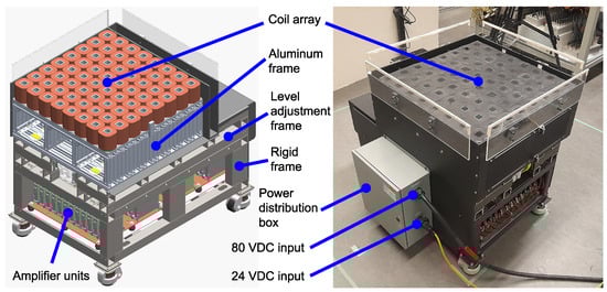
Figure 1.
Modular planar maglev system.
The lower part is a steel support structure. The structure has two layers: a level adjustment mechanism and a rigid frame. The level adjustment frame is used to adjust the position and level of the coil array mounting on the top. The rigid frame is welded. The frame has a built-in current amplifier module. The module is an assembly of 32 industrial drives installed on a copper plate for power return. The drive unit is a PWM current amplifier. It has a custom firmware that can power two coils separately. The drive unit requires two power inputs: 80 VDC 10 A maximum for the input supply and 24 VDC for the logic supply. The output is 80 VDC and 9 A maximum for each coil.
The system diagram is shown in Figure 2. Four five-megapixel cameras are placed at each corner above the system. The field of view is set to cover the entire area with a reference at the center of the coil array top surface. All cameras are connected to a switch with Power over Ethernet + (PoE+). These cameras are used to capture the reflective markers on the mover. The captured data are sent to the motion tracking software via Ethernet for mover pose computation. The mover pose is transmitted to the main controller to compute for control outputs. The current command outputs are assigned to the amplifiers via EtherCAT. EtherCAT is a high-speed communication protocol via a single cable. This protocol significantly simplifies the wiring from the controller to the amplifier units.
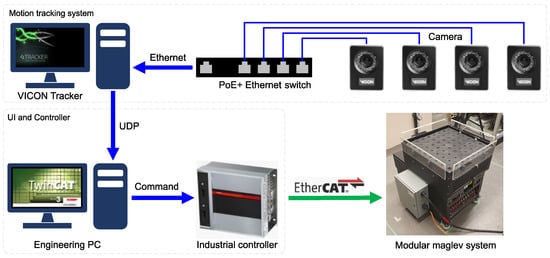
Figure 2.
Modular planar maglev system: hardware diagram.
2.2. Disc Magnet Movers
There are two movers in this work: single-disc and multiple-disc magnet movers. The mover design process is similar to that in [29]. For a single-disc magnet, disc magnets with 2-inch, 3-inch, and 4-inch diameters and 1/2-inch thickness were evaluated. From analysis, the condition number tends to be lower when the disc magnet has larger diameter compared to the coil width. Hence, a 4-inch Neodymium disc magnet grade N50 with remanence T was selected, as shown in Figure 3a. However, the single-disc magnet mover can only be controlled for 5-DOF motion without yaw rotation due to its symmetry about the vertical axis.
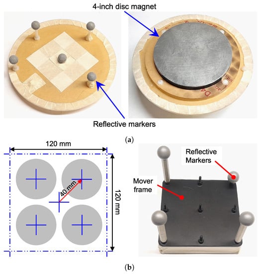
Figure 3.
Disc-magnet movers. (a) Single 4-inch disc magnet. (b) Four 2-inch disc magnets.
Next, the mover with multiple-disc magnets was designed to achieve 6-DOF motion. As shown in Figure 3b, the mover comprises four 2-inch disc magnets. The magnet is a Neodymium disc magnet grade N52 with remanence T. The magnet layout is optimized by considering three parameters: condition number, maximum current, and total power consumption. From the analysis, the layout with a diagonal distance of 40 mm was selected.
Both mover frames are acrylic and have reflective markers for motion tracking. There are three main markers at the same height for coordinate reference. Additional markers are mounted at different heights to prevent pose redundancy in motion tracking software. The mover coordinate is set at the center of the mover frame for both movers. The properties of both movers, mass and moments of inertia (I) about the x, y, and z axes of the mover coordinate, are shown in Table 1.

Table 1.
Mass properties of the designed movers.
3. Lorentz Levitation Modeling
3.1. Coordinate System Settings
In general, the planar magnetic levitation system consists of three main coordinate systems, as shown in Figure 4, as follows:

Figure 4.
Coordinate systems: system coordinate or origin {o}, coil coordinate {c}, and magnet coordinate {m}.
- {o}
- System coordinate or origin: located at the center of the coil array top surface;
- {c}
- Coil coordinate: located at the center of the coil top surface (ci for coil number i);
- {m}
- Magnet coordinate: located at the center of the magnet.
The planar coil array has 16 square coils arranged in a four-by-four pattern with the system origin o at the center of the coil array top surface. The disc magnet center m is levitated above the array with displacement , and orientation consists of rotation angles about the x (roll, ), y (pitch, ), and z (yaw, ) axes. The position of the coil number i referred to the origin is denoted by . Point a represents an arbitrary point of interest in the coil. Point a in coil number i coordinate is denoted by . This point is denoted by when referred to the origin. The vector is the position of point a relative to the center of the magnet.
3.2. Lorentz Wrench Model
For the 3-D forces and torques or wrench model for Lorentz levitation, this section describes the wrench model between a single coil with current density J immersed in the magnetic field B generated by a single magnet. The 3-D Lorentz wrench on the magnet can be expressed by
The computation has two challenges: the magnetic flux density and volume integral. Similar to [29,31], the magnetic nodes method is used to model the disc magnet and compute the magnetic flux density. The mover orientation is also considered since the magnet is freely levitated in the air. Next, this paper adopts the Gaussian quadrature technique, which was presented in [30], to approximate the triple integral as discrete summations by defining Gaussian nodes and weights on the coil.
3.3. Magnetic Flux Density Computation
By using the magnetic nodes, as detailed in [29], the disc magnet is modeled with nodes on the circumference of the top and bottom surfaces. The magnetic flux density at any points of interest in the mover coordinate is denoted by . To compute magnetic flux density at point a in the mover coordinate, the point a of coil i in system coordinate must be transformed into mover coordinate by
The magnet orientation has three rotation angles . The order of rotation is considered in yaw ()–pitch ()–roll (), as presented by
The disc magnet bottom () and top () surfaces have M magnetic nodes with remanence . The magnetic flux density in magnet coordinate from each magnetic node at the point a of coil i, , can be computed via
Finally, the magnetic field in the system coordinate can be obtained by transforming the magnetic field in the magnet coordinate back to the system coordinate by
The magnetic flux density from the magnet mover to any points of interest can be computed. This is further used to compute the Lorentz forces and torques on the magnet from each coil immersed in the magnetic field.
3.4. Numerical Integration for Wrench Model
To simplify the volume integral, the Gaussian quadrature technique is applied to approximate the integral as the summation of the functions by
In this work, the lower limit and upper limit of the integral are dimensions of a rounded-corner square coil which has height , inner corner radius , outer corner radius , and winding thickness . Similarly to [30], the coil is divided into eight sections : four rectangle and four rounded-corner sections. Each coil section is modeled to have Gaussian nodes n distributed at a specific location in all directions, or nodes in total. Each node has specific weight and current density J flowing in a counter-clockwise direction by default to provide +Z magnetization.
For the rectangle section, the wrench can be computed via
For the rounded corner section, the wrench can be computed via
By substituting magnetic flux density from Equations (5) and (6) into force and torque Equations (8) to (11), the wrench on the magnet can be computed via
where r is the moment arm from the magnet center p to the coil node n in system coordinate expressed by
The Lorentz force-based wrench model obtained in this section is further used for wrench–current decoupling in the next section.
4. Control System and Wrench–Current Decoupling for Long-Range Motion
4.1. Overall Control System
Figure 5 depicts an overall diagram of multi-DOF control for the planar maglev system. As mentioned in the system description, the mover motion is captured by the motion tracking system. The captured data are filtered and computed for the mover pose in the motion tracking software. Then, the mover pose and pose commands are fed to the multi-DOF controller to compute the controller commands.
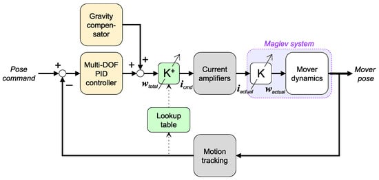
Figure 5.
Multi-DOF control diagram.
The Proportional–Integral–Derivative or PID control parameters for the 5-DOF control of a single-disc magnet mover and the 6-DOF control of a multiple-disc magnet mover are shown in Table 2. Since the weight of both movers is comparable, most of the PID parameters in both translations and rotations are similar. Only the D gains for roll and pitch angle and PID control for yaw rotation of the multiple-disc magnet mover were tuned.
Table 2.
Multi-DOF PID controller gains.
Next, the total desired wrench is a summation of the controller outputs and the gravity compensation. The compensator provides force in the z direction to partially support the vertical motion. This total wrench must be converted to currents for all active coils. However, it is difficult to determine the currents because the system has a strong cross-coupling effect in current-to-wrench transformation. The relationship between the wrench on the mover and the currents from all active coils can be represented by the wrench matrix :
The wrench matrix consists of the wrench vectors for n active coils. The components of the vector are the ratio of force f and torque to the current input of a single coil. The number of rows is the number of degrees of freedom. The number of columns is the number of coils. Since one coil current input can result in the 3-D wrench on the mover, the cross-coupling problem must be addressed to determine the coil current commands.
4.2. Wrench–Current Decoupling
As reviewed in the literature, one solution for the cross-coupling effect is to use the decoupling matrix. Generally, the decoupling matrix is an inverse of the wrench matrix. By implementing this matrix in the control system, the Multiple-Input Multiple-Output (MIMO) coupled system can be decoupled into multiple Single-Input Single-Output (SISO) systems. As a result, the motion in each degree of freedom can be controlled individually.
In this work, a block of the decoupling matrix, denoted by , is placed after the total desired wrench command , as shown in Figure 5. The matrix product is the coil current commands . All coil current commands are assigned to all active coils to attain the desired 3-D wrench on the mover. Suppose that the current amplifiers are ideal. Then, the actual currents can be produced as assigned from the controller or . Hence, the actual current in Equation (15) can be substituted by the decoupling matrix and total wrench commands as follows:
To realize , the decoupling matrix must be a right inverse of the wrench matrix K to fulfill the condition , where is an identity matrix. Usually, the number of active coils is more than the mover’s degrees of freedom. Hence, the wrench matrix is a nonsquare matrix. By using the Moore–Penrose pseudoinverse, the decoupling matrix or a right inverse of the wrench matrix can be obtained via
In the control system, the decoupling matrix must be obtained within the control sampling time of 1 ms. The lookup table method is used for real-time wrench–current decoupling. The lookup data are the wrench matrices for specific ranges of motion, which are computed in MATLAB with a parallel computing toolbox. The wrench matrix of the current pose can be obtained from the data and computed for the decoupling matrix.
4.3. Lookup Table
The lookup data ranges for a single-disc magnet mover and a multiple-disc magnet mover are detailed in Table 3. The total number of combinations for 5-DOF lookup data is 23,814 combinations. The total number of combinations for 6-DOF lookup data is 222,264 combinations. The data are converted to binary format and stored in the controller.
Table 3.
Lookup table data range for disc-magnet movers.
For translation, the XY data range for both movers is from 0 mm to 40 mm with an increment of 2 mm. This data range covers the first quadrant Q1 area in Figure 6b, which is the minimally repetitive planar area of this coil array pattern. For levitation height (Z), the single-disc magnet mover has a maximum height of 36.35 mm or a 30 mm air gap. The multiple-disc magnet mover has a lower maximum height at 30 mm or a 15 mm air gap.
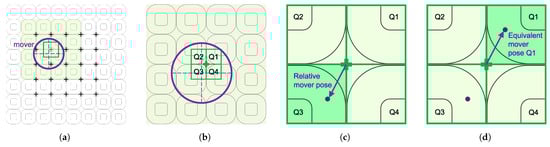
Figure 6.
Wrench–current decoupling strategy for long-range planar motion. (a) Find 4 × 4 active coils. (b) Find relative mover quadrant. (c) Find relative mover pose. (d) Find equivalent mover pose in Q1.
For rotation, both roll and pitch rotation range for both movers are from −10 degrees to 10 degrees with an increment of 10 degrees. For a multiple-disc magnet mover, the mover can rotate with the yaw angle. The yaw rotation data range is from 0 degrees to 90 degrees with a 15-degree increment step. In the lookup process, the reading yaw angle is calculated to find the equivalent yaw angle in the range of 0 to 90 degrees.
A multivariate linear interpolation was used to solve the discrete lookup data. For a single-disc magnet mover, 5-DOF linear interpolation can be formulated by determining the related indices from the mover pose: (, , , , ). The decoupling matrices are looked up using five state pairs , , , , , , , , and , . Therefore, 5-DOF interpolation requires = 32 matrices. For 6-DOF linear interpolation, the yaw angle is considered to determine a yaw state pair , . As a result, the number of lookup data becomes = 64 matrices.
4.4. Extended Wrench–Current Decoupling Data Using Quadrant Symmetry Transformation for Long-Range Planar Motion
The problem of the lookup table method with discrete lookup data was solved by multivariate linear interpolation to estimate the wrench–current decoupling matrix in the previous section. However, another remaining limitation of the lookup table method is a limited range of data, which limits the levitation range.
Since the memory used to store the lookup table data is directly proportional to the number of pose combinations, a larger range of levitation requires a larger size of lookup table. Therefore, a strategy to achieve long-range levitation with a small-range lookup table is needed for the efficient use of data memory.
In this research, the wrench–current decoupling technique for long-range motion using the minimum lookup data range is developed for the planar motor system. The number of active coils for levitation is 16 coils arranged in a four-by-four array. The lookup data are precomputed within the minimum planar range of the quarter coil area in the first quadrant of the coil array. Overall, the proposed strategy has four steps as follows:
STEP 1: Active coil array selection
Figure 6a depicts the concept of active coil array selection. The cross marks (+) represent the center of four-by-four active coils. The active coil array can be determined by the mover location. The 16 coils highlighted in green are the selected active coils for this mover pose since the center of this array is the nearest center to the mover.
For the planar maglev system in this work, the centers (, ) of all possible four-by-four active coil arrays in millimeter units are
The nearest active coil array center to the mover position (, ) can be determined by finding the coil center index (), which provides the minimum distance from
Once the active coil array center coordinate is determined from (, ) by the center index, all 16 active coils of the four-by-four coil array can be determined.
STEP 2: Pose transformation to the first quadrant (Q1)
From step 1, the relative mover pose (, ) to the relative quadrant (Qn) of the active coil array can be computed. Figure 6b represents that the mover is in the third quadrant (Q3) of the array. The relative mover pose to the coil array center is shown in Figure 6c.
Since the lookup data are only precomputed for Q1, the equivalent pose (, ) of the mover from other quadrants is transformed to Q1 via
where is the relationship between the x, y, and z components of another quadrant Qn to the first quadrant Q1. is a three-by-three zero matrix.
STEP 3: Lookup and interpolation for the wrench matrix
The lookup index can be computed via the equivalent pose in Q1 (, ) and looked up for the wrench matrix from the data table . An implementation of multivariate linear interpolation can be used to estimate the wrench matrix.
If multivariate linear interpolation is used, this step first computes all lookup indices and searches for all related states. Then, the estimated wrench matrix is computed as described in the previous section.
STEP 4: Wrench matrix transformation to the original quadrant (Qn)
Finally, the wrench matrix in the first quadrant is transformed back to the original quadrant. The wrench matrix in the original quadrant can be obtained by mapping the coil number or column number of the wrench matrix in Q1 to Qn and transforming the x, y, and z components of the wrench matrix by
The columns of are swapped by the column order for each original quadrant . The column order is obtained by rotating the coil number matrix degrees counter-clockwise and flattening the rotated matrix by row-major order as expressed by
Once the estimated wrench matrix is obtained, the estimated wrench–current decoupling matrix can be computed by using the Moore–Penrose pseudoinverse. An implementation of the developed algorithms on the controller has a computation time of less than 20 μs.
This section described the wrench–current decoupling strategy for long-range planar motion in the planar maglev system using short-range lookup data. This method is further evaluated on the planar maglev system in long-range levitation experiments.
5. System Setup and Experiment Results
5.1. System Setup
The system setup of the planar maglev system is shown in Figure 7a. Two power supply units with 80 and 24 VDC are connected to the system. Four optical cameras are set above the coil array to capture the mover pose. Each camera is 30 cm away from the corners of the coil array with different heights. All cameras connect to the Ethernet switch and motion tracking computer. The motion tracking system has a 1 kHz update rate with a resolution of ±10 μm and ±0.2 mrad. The controller operates the control algorithm and developed strategies with a 1 kHz sampling frequency. The current command is computed and sent out to the current amplifiers over the EtherCAT protocol.
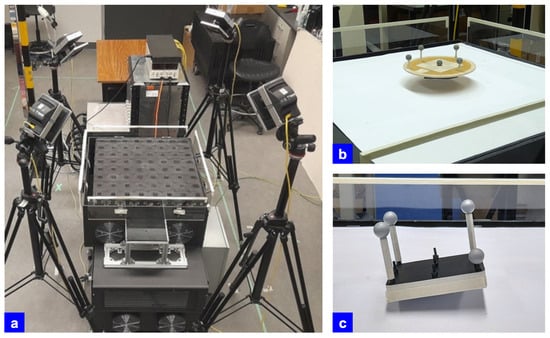
Figure 7.
Overall system setup and levitation. (a) System setup. (b) Single 4-inch disc mover levitation. (c) Four 2-inch disc mover levitation.
5.2. Experiment Results: Single 4-Inch Disc Magnet Mover
The experiment results on the planar maglev system with a single 4-inch disc magnet mover are presented in this section. The experiments consist of long-range motion in both translation and rotation. Figure 7b represents the mover levitating above the system. To demonstrate long-range levitation, the proposed long-range decoupling strategy was implemented. Two experiments were conducted. The first experiment is translation. The second experiment is rotations in both roll and pitch.
5.2.1. Long-Range Planar Motion
For translation, the planar motion stroke is ±190 mm with two levitation air gaps of 20 mm (26.35 mm) and 30 mm (36.35 mm). Figure 8a demonstrates the 3-D long-range translation over the coil array. The motions of other axes are plotted in Figure 8b. The 3-D translations are moved with ramp commands.
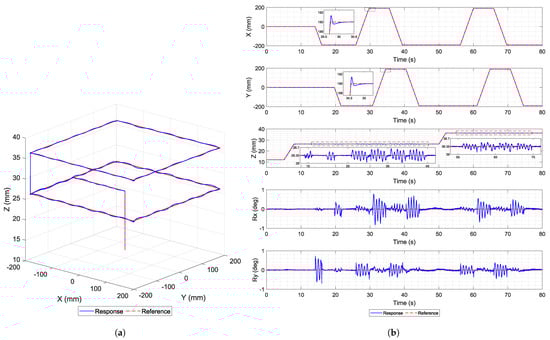
Figure 8.
Single 4-inch disc magnet mover: long-range translation. (a) 3-D. (b) All axis motion.
Meanwhile, the cross-coupling effect during the experiment in roll and pitch rotations can be observed with an error range of ±1 degree. For example, large oscillations in roll (Rx) motion occur when the mover moves along the y axis and vice versa.
5.2.2. Full-Range Rotation: Roll and Pitch
For rotation, the mover must be levitated with its center at z = 30 mm to avoid collision with the top surface of the coil array when the mover rotates at a large angle.
Then, the mover is rotated in place with roll and pitch angles of ±10 degrees, as shown in Figure 9. The trajectory tracking results in rotation demonstrate good tracking performance. However, the oscillations in the x, y, and z axes are ±0.07 mm. The cross-coupling effect between x–pitch and y–roll can still be observed in this experiment.
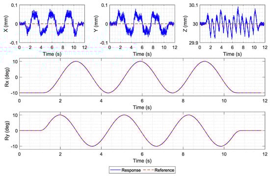
Figure 9.
Single 4-inch disc magnet mover: full-range roll and pitch 10-degree in-place rotation.
This section demonstrates the levitation performance of a single-disc magnet mover on a planar maglev system. With interpolation, large oscillations were suppressed when the mover levitated in the middle of lookup states, especially in rotations. By implementing a 5-DOF linear interpolation and decoupling strategy, the mover can move with smooth responses and be able to hover over the entire area of the coil array.
However, the remaining downside is yaw rotation. Uncontrolled yaw rotation can disturb the motion responses in other degrees of freedom. Levitation experiments using a multiple-disc magnet mover with yaw rotation are examined in the next section.
5.3. Experiment Results: Four 2-Inch Disc Magnet Mover
The experiment results on the planar maglev system with a four 2-inch disc magnet mover are presented in this section. Similar to a single-disc magnet, the experiments consist of long-range motion in both translation and rotation, including yaw rotation. Figure 7c represents the mover levitating above the system with roll and pitch angles.
To demonstrate the performance of long-range levitation and the implementation of the developed technique, two experiments were conducted. The first experiment is long-range translation. The second experiment is full-range rotation.
5.3.1. Long-Range Planar Motion
For trajectory tracking in translation, two motion paths are defined for experiments. The first long-range translation path is a planar motion of ±75 mm at z = 20 mm, as shown in Figure 10. The second long-range translation path is a planar motion of ±150 mm at z = 20 mm, as shown in Figure 11.
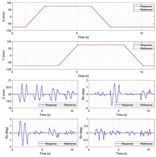
Figure 10.
Four 2-inch disc magnet mover: long-range translation, 150 mm.
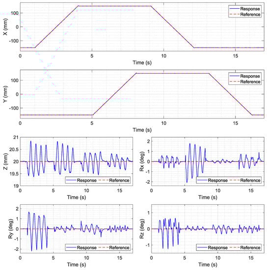
Figure 11.
Four 2-inch disc magnet mover: long-range translation, 300 mm.
For both long-range motions, the motion in the x and y axes can follow the ramp command. However, large oscillations occur on other axes when the mover is moving along the path. For z motion, the mover oscillates within the range of ±0.75 mm. The roll and pitch motions have large oscillations of ±2 degrees, and the range of the yaw motion is within ±0.5 degrees, except for the first part in the ±150 mm path. Most large oscillations emerge in the first half of the motion when the mover moves from −75 mm to 75 mm and from −150 mm to 150 mm along the x axis.
5.3.2. Full-Range Rotation: Roll and Pitch
To avoid the mover colliding with the top surface of the coil array when it rotates at the maximum roll or pitch angle, the mover center is levitated to z = 30 mm before rotation. For roll and pitch rotation, the experiment was conducted on in-place rotation.
The mover is rotated in place with ±10 degrees in both roll and pitch, as shown in Figure 12. The command tracking results demonstrate good tracking performance. The responses in other DOF are larger than those of the ramp command experiment. The errors in the x and y axes are ±0.06 mm, ±0.125 mm for the z axis, and ±0.2 deg for yaw rotation.
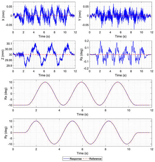
Figure 12.
Four 2-inch disc magnet mover: full-range roll and pitch 10-degree in-place rotation.
5.3.3. Full-Range Rotation: Yaw
For yaw rotation, the mover can become unstable when the mover rotates at the central region of the coil array, which consumes a high current. In this experiment, the mover is moved to (x, y) = (38.1, 0) at z = 16 mm before rotation. Then, the mover is controlled to rotate about the vertical axis from 0 to 360 degrees with an angular speed of 180 deg/s.
The full-range yaw rotation experiment was conducted with an angular speed of 180 deg/s. Figure 13a represents the yaw rotation result and error. Even though the mover was not rotated at the central region of the active coil array, large periodic errors of ±4 degrees in yaw motion can be observed at certain yaw angles.
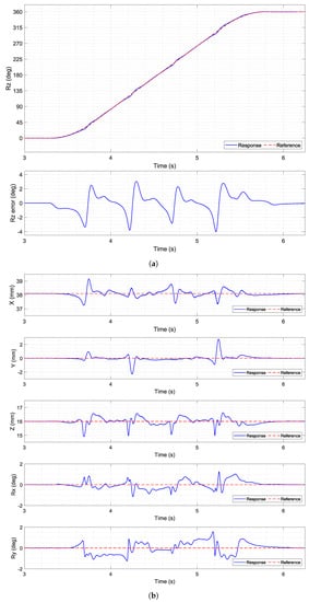
Figure 13.
Four 2-inch disc magnet mover: yaw rotation. (a) Yaw with error. (b) Other axes’ responses.
Meanwhile, large errors in other DOF during full-range yaw rotation can be observed in Figure 13b. In translation, several spikes occur in all axes periodically. For roll and pitch rotation, the error range is within ±1.5 degrees.
This section presents implementation and levitation experiments on the planar maglev system with a single 4-inch magnet mover and a four 2-inch magnet mover. By using the lookup table method, we can study decoupling performance when the mover is levitated at the middle of the lookup data, especially roll and pitch rotations. With an implementation of multivariate linear interpolation, the decoupling performance was significantly enhanced. The decoupling strategy using the quadrant symmetry transformation for long-range levitation was successfully implemented for both movers.
6. Discussion
The discussions of the proposed decoupling strategy and levitation experiment results are provided in this section.
The proposed technique for wrench–current decoupling in long-range motion utilizes minimally repetitive wrench data and quadrant symmetry transformation. The wrench data in this work are computed on a 40 mm-by-40 mm or a quarter area of a single coil in the first quadrant of a 16-coil array. By using the quadrant symmetry transformation, the data can be extended for unlimited planar translation. Even though the height, roll, and pitch angles are still limited, the maximum range can be determined from the levitation specifications. However, the minimally repetitive area depends on the pattern of the coil array. Therefore, the minimally repetitive area must be determined for different coil arrays.
The developed wrench–current decoupling technique was implemented on the planar maglev system and demonstrated through the experiment results. In long-range levitation experiments, the technique successfully enables the mover to hover over the coil array, although the levitation performance still needs improvement. Since the wrench data were computed from an ideal coil array arrangement, the real-time wrench–current decoupling in levitation can deteriorate due to arrangement errors throughout the array.
The results demonstrated better levitation performance of a single-disc magnet mover compared to that of a multiple-disc magnet mover. The single-disc magnet mover can only have 5-DOF motion with uncontrollable yaw. This undesired yaw can disturb overall performance. The multiple-disc magnet mover can have 6-DOF motion; however, the coil current computation at some poses may result in a high current on some coils. This may cause current saturation and disturb the levitation performance.
As discussed above, there are several research opportunities to improve the planar maglev system in this work, for example, a real-time solution to improve wrench–current decoupling in uncertain environments. The advanced control algorithm can be developed to handle the over-current problem, maintain stability, and improve levitation performance [32]. For precision motion, the system also has the capability to perform high-precision tasks. With the review in [33], the motion sensing system should be redesigned to provide precise motion data. Magnetic sensors such as Hall effect sensors can be embedded in the coil array for motion sensing [34].
7. Conclusions and Future Works
In this work, the wrench–current decoupling technique using the quadrant symmetry transformation was developed to extend the use of the lookup data on the minimally repetitive area for long-range planar motion. The lookup data have a horizontal range of 40 mm by 40 mm or the quarter area of the coil in the first quadrant of the coil array. The quadrant symmetry transformation was used to estimate the wrench matrix in other areas. Multivariate linear interpolation was used to solve the discrete data problem. The experiment results demonstrated the accomplishment of the developed technique for long-range motion with a maximum motion stroke of 380 mm. The mover can levitate with a large air gap of 30 mm for a single-disc magnet mover and 15 mm for a multiple-disc magnet mover. The rotation range for roll and pitch was ±10 degrees for both movers and 360 degrees yaw for the multiple-disc magnet mover.
Future work with this research will continue to improve the levitation performance in long-range motion for both translation and rotation. Analysis of multiple-magnet movers could be conducted to achieve better 6-DOF motion. The implementation of advanced control algorithms can be applied to the system to demonstrate real-world applications such as precision stages or multidirectional conveyor systems.
Author Contributions
Conceptualization, C.T. and M.B.K.; methodology, C.T.; software, C.T.; validation, C.T. and M.B.K.; formal analysis, C.T.; investigation, C.T.; resources, C.T.; data curation, C.T.; writing—original draft preparation, C.T.; writing—review and editing, M.B.K.; visualization, C.T.; supervision, M.B.K.; project administration, M.B.K.; funding acquisition, M.B.K. All authors have read and agreed to the published version of the manuscript.
Funding
This work was supported by the Canada Foundation for Innovation (CFI) and the Natural Sciences and Engineering Research Council of Canada (NSERC).
Institutional Review Board Statement
Not applicable.
Informed Consent Statement
Not applicable.
Data Availability Statement
Data are available from the authors upon request.
Conflicts of Interest
The authors declare no conflict of interest.
References
- Lee, H.W.; Kim, K.C.; Lee, J. Review of maglev train technologies. IEEE Trans. Magn. 2006, 42, 1917–1925. [Google Scholar] [CrossRef]
- Nøland, J.K. Prospects and challenges of the hyperloop transportation system: A systematic technology review. IEEE Access 2021, 9, 28439–28458. [Google Scholar] [CrossRef]
- Abbott, J.J.; Diller, E.; Petruska, A.J. Magnetic Methods in Robotics. Annu. Rev. Control Robot. Auton. Syst. 2020, 3, 57–90. [Google Scholar] [CrossRef]
- Kummer, M.P.; Abbott, J.J.; Kratochvil, B.E.; Borer, R.; Sengul, A.; Nelson, B.J. OctoMag: An electromagnetic system for 5-DOF wireless micromanipulation. IEEE Trans. Robot. 2010, 26, 1006–1017. [Google Scholar] [CrossRef]
- Xu, T.; Zhang, J.; Salehizadeh, M.; Onaizah, O.; Diller, E. Millimeter-scale flexible robots with programmable three-dimensional magnetization and motions. Sci. Robot. 2019, 4, eaav4494. [Google Scholar] [CrossRef]
- Lim, A.; Schonewille, A.; Forbrigger, C.; Looi, T.; Drake, J.; Diller, E. Design and Comparison of Magnetically-Actuated Dexterous Forceps Instruments for Neuroendoscopy. IEEE Trans. Biomed. Eng. 2021, 68, 846–856. [Google Scholar] [CrossRef]
- Pedram, S.A.; Klatzky, R.L.; Berkelman, P. Torque Contribution to Haptic Rendering of Virtual Textures. IEEE Trans. Haptics 2017, 10, 567–579. [Google Scholar] [CrossRef]
- Smirnov, A.; Uzhegov, N.; Sillanpää, T.; Pyrhönen, J.; Pyrhönen, O. High-speed electrical machine with active magnetic bearing system optimization. IEEE Trans. Ind. Electron. 2017, 64, 9876–9885. [Google Scholar] [CrossRef]
- Pisetskiy, S.; Kermani, M. High-Performance Magneto-Rheological Clutches for Direct-Drive Actuation: Design and Development. J. Intell. Mater. Syst. Struct. 2021, 32, 2582–2600. [Google Scholar] [CrossRef]
- Wang, S.; Li, H.; Yuan, D.; Wang, S.; Wang, S.; Zhu, T.; Zhu, J. Oscillations and size control of Titanium droplet for electromagnetic levitation melting. IEEE Trans. Magn. 2018, 54, 1–4. [Google Scholar] [CrossRef]
- Kumar, P.; Ansari, M.; Toyserkani, E.; Khamesee, M.B. Experimental implementation of a magnetic levitation system for laser-directed energy deposition via powder feeding additive manufacturing applications. Actuators 2023, 12, 244. [Google Scholar] [CrossRef]
- Kim, W.J.; Trumper, D.L. High-precision magnetic levitation stage for photolithography. Precis. Eng. 1998, 22, 66–77. [Google Scholar] [CrossRef]
- Verma, S.; Kim, W.J.; Shakir, H. Multi-axis maglev nanopositioner for precision manufacturing and manipulation applications. IEEE Trans. Ind. Appl. 2005, 41, 1159–1167. [Google Scholar] [CrossRef]
- Kim, W.J.; Verma, S.; Shakir, H. Design and precision construction of novel magnetic-levitation-based multi-axis nanoscale positioning systems. Precis. Eng. 2007, 31, 337–350. [Google Scholar] [CrossRef]
- Schaeffel, C.; Katzschmann, M.; Mohr, H.; Gloess, R.; Rudolf, C.; Mock, C.; Walenda, C. 6D planar magnetic levitation system - PIMag 6D. Mech. Eng. J. 2016, 3, 15-00111. [Google Scholar] [CrossRef][Green Version]
- Zhu, H.; Teo, T.J.; Pang, C.K. Design and modeling of a six-degree-of-freedom magnetically levitated positioner using square coils and 1-D Halbach arrays. IEEE Trans. Ind. Electron. 2017, 64, 440–450. [Google Scholar] [CrossRef]
- Zhu, H.; Teo, T.J.; Pang, C.K. Magnetically levitated parallel actuated dual-Stage (Maglev-PAD) system for six-axis precision positioning. IEEE/ASME Trans. Mechatron. 2019, 24, 1829–1838. [Google Scholar] [CrossRef]
- Dyck, M.; Lu, X.; Altintas, Y. Magnetically Levitated Rotary Table With Six Degrees of Freedom. IEEE/ASME Trans. Mechatron. 2017, 22, 530–540. [Google Scholar] [CrossRef]
- Xu, F.; Zhang, K.; Xu, X. Development of magnetically levitated rotary table for repetitive trajectory tracking. Sensors 2022, 22, 4270. [Google Scholar] [CrossRef]
- Lu, X.; Usman, I. 6D direct-drive technology for planar motion stages. CIRP Ann. Manuf. Technol. 2012, 61, 359–362. [Google Scholar] [CrossRef]
- Gloess, R. Mag-6D a new mechatronics design of a levitation stage with nanometer resolution. In Proceedings of the 31st ASPE Annual Meeting 2016, Portland, OR, USA, 23–28 October 2016; pp. 423–427. [Google Scholar]
- Jansen, J.W.; van Lierop, C.M.M.; Lomonova, E.A.; Vandenput, A.J.A. Magnetically levitated planar actuator with moving magnets. IEEE Trans. Ind. Appl. 2008, 44, 1108–1115. [Google Scholar] [CrossRef]
- Berkelman, P.; Dzadovsky, M. Single magnet levitation by repulsion using a planar coil array. In Proceedings of the 2008 IEEE International Conference on Control Applications, San Antonio, TX, USA, 3–5 September 2008; pp. 108–113. [Google Scholar] [CrossRef]
- Berkelman, P.; Dzadovsky, M. Magnetic levitation over large translation and rotation ranges in all directions. IEEE/ASME Trans. Mechatron. 2013, 18, 44–52. [Google Scholar] [CrossRef]
- Miyasaka, M.; Berkelman, P. Magnetic levitation with unlimited omnidirectional rotation range. Mechatronics 2014, 24, 252–264. [Google Scholar] [CrossRef]
- Hollis, R.L.; Salcudean, S.E. Lorentz levitation technology: A new approach to fine motion robotics, teleoperation, haptic interfaces, and vibration isolation. In Proceedings of the International Symposium on Robotics Research, Kyoto, Japan, 28–30 October 1993. [Google Scholar]
- Bancel, F. Magnetic nodes. J. Phys. Appl. Phys. 1999, 32, 2155–2161. [Google Scholar] [CrossRef]
- Xu, Z.; Zhang, X.; Khamesee, M.B. Real-time data-driven force and torque modeling on a 2-D Halbach array by a symmetric coil considering end effect. IEEE Trans. Magn. 2022, 58, 1–10. [Google Scholar] [CrossRef]
- Zhang, X.; Trakarnchaiyo, C.; Zhang, H.; Khamesee, M.B. MagTable: A tabletop system for 6-DOF large range and completely contactless operation using magnetic levitation. Mechatronics 2021, 77, 102600. [Google Scholar] [CrossRef]
- Xu, F.; Lv, Y.; Xu, X.; Dinavahi, V. FPGA-based real-time wrench model of direct current driven magnetic levitation actuator. IEEE Trans. Ind. Electron. 2018, 65, 9635–9645. [Google Scholar] [CrossRef]
- Trakarnchaiyo, C.; Wang, Y.; Khamesee, M.B. Design of a Compact Planar Magnetic Levitation System with Wrench–Current Decoupling Enhancement. Appl. Sci. 2023, 13, 2370. [Google Scholar] [CrossRef]
- Li, X.; Zhu, H.; Ma, J.; Teo, T.J.; Teo, C.S.; Tomizuka, M.; Lee, T.H. Data-Driven Multiobjective Controller Optimization for a Magnetically Levitated Nanopositioning System. IEEE/ASME Trans. Mechatron. 2020, 25, 1961–1970. [Google Scholar] [CrossRef]
- Zhou, L.; Wu, J. Magnetic Levitation Technology for Precision Motion Systems: A Review and Future Perspectives. Int. J. Autom. Technol. 2022, 16, 386–402. [Google Scholar] [CrossRef]
- Yu, H.; Kim, W.J. A Compact Hall-Effect-Sensing 6-DOF Precision Positioner. IEEE/ASME Trans. Mechatron. 2010, 15, 982–985. [Google Scholar] [CrossRef]
Disclaimer/Publisher’s Note: The statements, opinions and data contained in all publications are solely those of the individual author(s) and contributor(s) and not of MDPI and/or the editor(s). MDPI and/or the editor(s) disclaim responsibility for any injury to people or property resulting from any ideas, methods, instructions or products referred to in the content. |
© 2023 by the authors. Licensee MDPI, Basel, Switzerland. This article is an open access article distributed under the terms and conditions of the Creative Commons Attribution (CC BY) license (https://creativecommons.org/licenses/by/4.0/).