An Efficient and High-Precision Electromagnetic–Thermal Bidirectional Coupling Reduced-Order Solution Model for Permanent Magnet Synchronous Motors

Abstract

The traditional electromagnetic–thermal bidirectional coupling model (EMTBCM) of permanent magnet synchronous motors (PMSMs) requires a long time to solve, and the temperature-induced torque change is not accounted for in the finite element (FE) numerical calculation of the EM field. This paper presents a precise and efficient EMTBC reduced-order solution model. The specific methods are as follows: First, a torque control technology based on the current injection method is proposed for determining the effect of temperature on the properties of EM materials and EM torque in an EM field, and the accuracy of the FE numerical calculation model is improved. Second, we use the improved EM field finite element numerical calculation model (FEMNCM) to analyze the correlation between the EM loss, the temperature, and the load, and we replace the FEMNCM with the EM field reduction model using the least-squares method. Then, we analyze the law of the PMSM’s internal temperature distribution. We choose the GA-BP algorithm with as few samples as possible and a high accuracy and stability to build the regression prediction model of the temperature field. We use this regression prediction model to replace the complex temperature field calculation. After analyzing the EMTBCM solution strategy, the original complex EMTBC numerical calculation model is substituted with iterations of the magnetic field reduction model and the temperature field regression prediction model. The FE numerical calculation is then used to validate the reduced-order model. The proposed model is validated through numerical simulations. The numerical results indicate that the proposed reduced-order EMTBC model in this paper is accurate and computationally efficient.

1. Introduction

As an electric drive permanent magnet synchronous motor (PMSM) has a small size, large torque, wide speed regulation range, high power density, and high efficiency, it has been extensively utilized [1,2] in a variety of applications. In the design of PMSMs, thermodynamic optimization is equally as essential as electromagnetic (EM) optimization, because the performance of the motor is not only determined by the EM performance but also strongly influenced by the temperature field [3]. Temperature increase is a significant factor that impedes motor miniaturization and high-power density, so it is essential to have temperature data for the motor’s overall design and online monitoring. Due to the aforementioned factors, it is crucial to develop an accurate and efficient thermal calculation model for the multi-physics design of PMSMs.

Various thermal analysis methodologies for electric motors have been proposed in recent years. The lumped parameter thermal network method concentrates the source of heat loss on each discrete node, connects the nodes through thermal resistance, and then establishes the network topology relationship according to the direction and path of heat transfer within the motor, which significantly reduces the computation time [4,5]. The adopted lumped parameter thermal network method analyzes the temperature field of the motor [6], and the lumped parameter thermal network method has a high calculation efficiency. However, it can only determine the average temperature of the motor and cannot determine the temperatures of individual components. Moreover, owing to the equivalence and approximation of the thermal resistance network construction procedure, the calculation results of the lumped parameter thermal loop lack precision, so the lumped parameter thermal network method is not considered in this paper.

For the calculation of motor temperature rise, there are two primary methods: the unidirectional coupling calculation method [7] and the bidirectional coupling calculation method [8]. The numerical calculation for unidirectional coupling directly couples the EM field loss to the temperature field. Since the electrical resistivity of the copper wire of the motor increases as the motor temperature rises and the remanence of the PM decreases as the temperature rises, the unidirectional coupling calculation method in the EM field does not account for the temperature characteristics of the EM material. Therefore, this motor temperature calculation procedure is inaccurate [9]. The EMTBC numerical calculation incorporates EM field loss data into the temperature field, while temperature field data are transferred to the EM field. This calculation method considers the effect of temperature on the properties of EM materials and enhances the precision of temperature rise calculations [10,11]. Comparing the temperature rise calculation results of the EM-thermal unidirectional coupling method and the EMTBC method, numerical calculations and experimental results demonstrate that the EMTBC method provides more accurate calculations [12].

Even though the PMSM method for solving the temperature field with EMTBC has a high level of accuracy, the iterative process of the EM field and temperature field requires a great deal of calculation time, which is clearly insufficient to meet the demand for high thermal calculation efficiency. Alternatively, during the actual operation of the motor, when the PM is demagnetized, the controller autonomously adjusts the power angle to maintain torque [13]. Nonetheless, in the process of the EMTBC numerical calculation, the increase in temperature reduces the remanence of the PM, but the power angle of the EM field does not change automatically, resulting in a reduction in accuracy; therefore, it is necessary to propose a new methodology to further consider the adaptive control of torque.

In this paper, a high-precision reduced-order EMTBC solution model is proposed to address the computational issue of the traditional EMTBC model. Our strategies include the following: First, the effect of temperature variations on the EM torque is considered. Then, the stability of the EM torque is regulated by temperature feedback, as well as control methods. (In this way, the temperature accuracy of the solution through the EMTBC will be greatly improved). Secondly, the EM field and temperature field are calculated, and their respective reduced-order calculation models are then established based on the results of the calculations. (The aim is to replace the calculation of EM and temperature fields with proxy modeling). Thirdly, the two established one-dimensional models are coupled iteratively in accordance with the bidirectional coupling solution strategy to simulate the bidirectional EM-thermal coupling solution process. (With the progress of the bidirectional coupling iteration, the obtained temperature value will be closer to the real value). Finally, a finite element analysis (FEA) is used to validate the results of our proposed method.

2. Theoretical Analysis

2.1. Theoretical Analysis of Demagnetization of PM

Since PMs have a high temperature coefficient, their remanence (B) and coercivity (Hci) vary as the temperature changes. The temperature coefficient α_Br quantifies the extent to which the residual magnetic induction intensity of PM materials can be reversibly altered by temperature, and the unit is K⁻¹ [14].

$${\alpha }_{Br}=\frac{B_1-B_0}{B_0(t_1-t_0)}\times 100$$

(1)

Similarly, α_Hci is also commonly used to represent the degree to which the intrinsic coercivity of PM materials changes reversibly with temperature, in K⁻¹ [14].

$${\alpha }_{Hci}=\frac{Hc{i}_1-Hc{i}_0}{Hc{i}_0(t_1-t_0)}\times 100$$

(2)

where B₀, B₁ and Hci₀, Hci₁ are the values at temperatures t₀ and t₁, respectively.

Equations (1) and (2) demonstrate that both the remanence and coercivity of the PM decrease as the temperature rises. Consequently, the influence of temperature rise on the properties of EM materials must be accounted for in the calculation of the motor temperature rise via the mutual coupling iteration of the EM field and temperature field.

As demonstrated in (3), for the irreversible magnetization loss of the PMSM, because the remanence (B) decreases, this leads to a decrease in B_r and B_ɵ, which further leads to a decrease in the motor drive torque [15].

$$T_{em}=\frac{L_{ef}}{{\mathsf{\mu }}_0}{\displaystyle \oint r^2{B}_r{B}_{\theta }d\theta }$$

(3)

where r is the radius of any circle located in the air gap; B_r and B_ɵ are the radial and tangential components of the magnetic density of the air gap at radius r. L_ef calculates the length of the armature.

When magnetic pole i loses magnetic K_i (K_i denotes the percentage of the ith pole demagnetization), the winding back electromotive force (Back-EMF) of the motor also changes [16].

$$\begin{array}{l}{e}_{si}{}_{,A1}(t)=E_s(1-\frac{K_i}{2p})\sin (2\pi f_{e}t-\frac{\pi }{6})-E_s{K}_i{\displaystyle {\sum }_{k=1}^{\infty }\frac{1}{k\pi }\sin (\frac{k\pi }{2p})}\cdot \\ \sin [2\pi f_{e}t(1\pm \frac{k}{p})\mp \frac{(3i-1)k\pi }{3p}-\frac{\pi }{6}]\end{array}$$

(4)

where e_si is the Back-EMF of a single-slot winding group during no-load operation at the rated motor speed, E_s is the no-load fundamental wave Back-EMF amplitude of a single slot, 2p is the number of poles, and A1 represents the first slot of the A-phase winding.

Equation (4) demonstrates that, when the magnetic pole is demagnetized, the value of the Back-EMF decreases, which causes the winding current to increase.

In summary, a reduction in the PM’s remanence further diminishes the motor’s torque. In order to maintain a constant EM torque, the closed-loop controller increases the winding current. Therefore, if the PM is demagnetized during actual motor operation, the winding current increases to compensate for the magnetic density amplitude of the PM. In the numerical calculation of the conventional EMTBC, however, only the influence of temperature on the EM material is considered; however, the torque variation due to the influence of temperature increase must also be considered.

2.2. Loss Analysis

2.2.1. Core Loss

Iron loss accounts for the majority of PMSM losses. The formula for calculating the iron core loss is as follows [17]:

$$p_{fe}=p_h+p_c+p_a=k_{h}f{B}_m^{\alpha }+k_c{f}^2{B}_m^2+k_a{f}^{1.5}{B}_m^{1.5}$$

(5)

Since the resistivity of ferromagnetic materials is affected by temperature and increases as the temperature rises, the resistivity of ferromagnetic materials increases [18,19].

$$\rho (T)=\rho (20)(1+k_t\cdot (T-20))$$

(6)

where T is the temperature, ρ(20) is the resistivity at room temperature, T = 20 °C, and, finally, k_t denotes the temperature coefficient.

Therefore, a temperature coefficient, k_t, is introduced to characterize the effect of temperature on the eddy current loss term. By substituting Equation (6) into the expression for the eddy current loss coefficient, it can be deduced [18,19]:

$$p_{fe}=p_h+p_c+p_a=k_{h}f{B}_m^{\alpha }+\frac{k_c}{1+k_t(T-20)}{f}^2{B}_m^2+k_a{f}^{1.5}{B}_m^{1.5}$$

(7)

where p_h is the hysteresis loss. p_c is the eddy current loss. p_a is the abnormal eddy current loss. B_m is the magnetic density amplitude of the iron core. f is the frequency. k_h is the hysteresis loss coefficient. k_c is the abnormal eddy current loss coefficient, k_a is the additional loss coefficient, and α is the Steinmetz coefficient. The standard electric steel loss factors (k_h, k_c, k_a) are used in this paper.

2.2.2. Copper Loss

The copper loss p_Cu of the PMSM can be expressed as follows [20]:

$$P_{cu}=m{I}^{2}R$$

(8)

where m is the number of phases, I is the effective value of the phase current, and R is the phase resistance.

The resistance of copper is shown in Equation (7):

$$R=\rho \frac{L}{S}$$

(9)

where ρ is the resistivity of copper.

Since the resistivity of copper varies with temperature, the following expression is valid [20]:

$$\rho ={\rho }_0[1+\alpha (t-t_0)]$$

(10)

where α is the resistance temperature coefficient of the material.

Because a low-speed motor is utilized in this study, the AC loss and mechanical loss are not taken into account in this work.

3. Methodologies

A high-power-density and compactly designed PMSM is extremely demanding, but these characteristics make motor heat dissipation difficult to design. An improper thermal design of a motor can result in an excessive internal temperature rise and failure. Obtaining accurate temperature field calculation results for motor thermal design, nevertheless, is a time-consuming process. Therefore, we proposed a method for EMTBC dimensionality reduction in order to develop an effective and high-precision model for the solution. The strategy is depicted in Figure 1.

3.1. Finite Element Model (FEM)

This article utilizes a 1.5 kW surface-mounted PMSM as its research subject. The motor’s specifications are listed in

Table 1. Specifications of the adopted motor.

Parameter	Value	Parameter	Value
Rated output power	1.5 KW	Rated speed	3000 r/min
Length	40 mm	Number of poles (2p)	8
Stator outer diameter	120 mm	Number of slots (Q)	12
Stator inner diameter	80 mm	Magnet thickness	4 mm
Rotor outer diameter	79 mm	air gap	0.5 mm
Rated frequency	50 Hz	PM material	N38H

. The motor’s PM type is N38H, its winding insulation is class B, its maximum operating temperature is 130 °C, and its cooling structure is air-cooled. Because the PMSM is a symmetrical structure, the 1/4 model is chosen to determine the transient magnetic field in order to reduce the calculation time. Figure 2a depicts the mesh partitioning for the simulation investigation. Figure 2b depicts the motor architecture.

3.2. Enhancement of EM Field FEM

Using the traditional EMTBC method to solve the temperature field, the remanence of the PM diminishes as the temperature increases, and the torque also decreases. Figure 3 displays the calculated motor torque at various temperatures. In the numerical calculation, one can see that an increase in temperature decreases the EM torque of the motor, and the higher the temperature, the greater the torque decrease.

To maintain a constant EM torque under the EMTBC solution model, a torque control method based on the current injection technique is proposed. The fundamental concept is to increase the input current as the temperature rises and to maintain a constant torque by increasing the magnetic field intensity. Consequently, this paper employs a numerical calculation method to ascertain the temperature and current change under a constant torque, and then it fits the corresponding relationship between the temperature and current under a varying torque. By controlling the change in the current value during the EMTBC procedure, it is intended to prevent the EM torque from varying with the temperature rise.

Table 2. Corresponding table of change in temperature and current under constant torque.

Temperature (℃)	Current at Different Temperatures at Rated Torque (A)	Current at Different Temperatures at 1.25 Times Torque (A)	Current at Different Temperatures at 1.5 Times Torque (A)	Current at Different Temperatures at 1.75 Times Torque (A)	Current at Different Temperatures at 2 Times Torque (A)
20	10	13.55	17.16	20.68	24.32
30	10.32	13.89	17.55	21.07	24.72
40	10.62	14.23	17.9	21.46	25.12
50	10.93	14.56	18.26	21.85	25.54
60	11.26	14.89	18.62	22.25	25.96
70	11.58	15.24	18.99	22.65	26.39
80		15.58	19.38	23.06	26.82
90			19.79	23.49	27.26
100				23.92	27.71
110					28.17

contains the numerical results. It is important to note that, as the output torque increases, the temperature of each motor component also increases. We determined the solution method of the intermediate gradient change in Table 2 by calculating the maximum temperature rise under various torques.

The data in

Table 3. Effect of load on EM loss.

Current (A)	Iron Loss (W)	Eddy Current Loss of PM (W)	Copper Loss (W)
13.89	64.19	6.30	8.27
17.55	65.53	6.62	23.94
21.07	65.71	7.05	34.47
24.72	66.15	7.63	47.45

are fitted using the least-squares method, with the current serving as the dependent variable and the temperature and torque serving as the independent variables. Figure 4 depicts the results, and the following equation can be used to calculate the current value under arbitrary torque and temperature conditions:

$$\mathrm{z}=\mathrm{z}0+a\mathrm{x}+b\mathrm{y}+c{\mathrm{x}}^2+d{\mathrm{y}}^2+f\mathrm{xy}$$

(11)

In the equation, z represents the current, x represents the temperature, y represents the torque, z0 = −4.6636, a = 0.01812, b = 3.13168, c = 0.0000314481, d = −0.0000902057, and f = 0.0023. When R² = 0.99999, this indicates that the fitting effect is good.

If the output torque is known, the feedback temperature value can be used to modify the current value during the EMTBC to maintain a constant torque. To verify the efficacy of the proposed control method, the FE numerical calculation was performed, as depicted in Figure 5.

Figure 5 is a comparison of torque simulations at various temperatures. Based on the comparison of the results, it is evident that the EMTBC temperature rise calculation after the control is implemented can keep the torque essentially constant (improving the accuracy of the temperature rise calculations), which further demonstrates the efficacy of the employed control method.

3.3. Solution of Reduced-Order Model of EM Loss

3.3.1. Influence of Load and Temperature on EM Loss

In the previous section, we proposed a new model to considerably improve the calculation efficiency of FEM in the EM field. This section employs this model for further analysis. PMSM has a wide operating load range, and the EM loss varies with varied loads. Alternatively, the temperature affects the remanence of the PM, which in turn modifies the load angle of the motor’s operation; consequently, the temperature also affects the loss. To numerically analyze the influence of the load and temperature rise on the EM loss of the motor, each parameter was sequentially altered within the predetermined range of the load and temperature. The effect of each parameter on the EM loss of the motor is illustrated in Table 3,

Table 4. Effect of temperature on EM loss.

Temperature (°C)	Iron Loss (W)	Eddy Current Loss of PM (W)	Copper Loss (W)
30	65.60	7.05	34.47
60	61.25	6.52	45.78
90	57.84	6.19	59.22
120	51.26	6.15	74.95

, and Figure 6.

As shown in Figure 6, the results show the following:

–

The iron loss increases with the increasing load current and decreases with the increasing temperature. This is because the increase in the current enhances the induced magnetic field of the stator, thus increasing the stator iron loss; however, the increase in the temperature reduces the remanent magnetic field of the PM, as well as the loss coefficient of the silicon steel sheet, thus decreasing the iron loss.

–

The copper loss increases with the increasing load current and temperature. However, the increasing temperature increasing the resistance of the copper wire leads to an increasing copper loss.

–

The eddy current loss of the PM increases with the increasing load current and decreases with the increasing temperature. The reason for this is that the increase in the load current enhances the working magnetic field of the PM, while the increase in the temperature reduces the remanent magnetic field of the PM. Therefore, the EM loss has a certain correlation with the load current and temperature.

3.3.2. The Specific Law of Load and Temperature Effects on EM Loss

In order to analyze the relationship between the EM loss, load current, and temperature, this section uses temperature and various load torques as independent simulation variables, and the iron loss and eddy current loss of the PM as dependent variables. Combined with the data in Table 2, the results of the FE simulation are shown in

Table 5. Influence of load and temperature on iron loss and eddy current loss of PM.

Temperature (°C)	Loss at Rated Torque (W)		Loss at 1.25 Times the Torque (W)		Loss at 1.5 Times the Torque (W)		Loss at 1.75 Times the Torque (W)		Loss at 2 Times the Torque (W)
	Iron Loss	PM Eddy Current Loss	Iron Loss	PM Eddy Current Loss	Iron Loss	PM Eddy Current	Iron Loss	PM Eddy Current Loss	Iron Loss	PM Eddy Current Loss
20	66.19	6.22	66.33	6.47	66.55	6.83	66.87	7.25	67.45	7.80
30	64.78	5.95	65.17	6.22	65.38	6.62	65.60	7.05	66.04	7.63
40	63.39	5.69	63.92	5.97	63.98	6.39	64.25	6.85	64.59	7.47
50	61.89	5.44	62.61	5.74	62.35	6.19	62.74	6.68	63.01	7.34
60	60.21	5.20	61.09	5.52	60.76	6.00	61.25	6.52	61.42	7.23
70	58.53	4.97	59.49	5.31	59.10	5.83	59.52	6.38	59.66	7.14
80			57.58	5.11	57.42	5.67	57.84	6.19	57.96	7.06
90					55.86	5.55	56.22	6.19	56.40	7.06
100							54.43	6.14	54.63	7.07
110									53.20	7.14

. In addition, since there is an error in the calculation of copper consumption in Maxwell (Maxwell calculates the resistance value from the cross-sectional area of the stator slots and the length of the stator, and it does not take into account the real winding structure), we manually compute the copper consumption of the windings.

In order to facilitate observation and acquire specific rules, polynomial fitting is performed using the least-squares method on Table 5 data. The effect of the fitting is illustrated in Figure 7. Equations (10)–(12) illustrate the specific principles of the load current, temperature, and iron consumption; the eddy current loss of the PM; and copper consumption. Consequently, the specific value of the EM loss can be calculated using the load current and temperature.

$$P_{iron\_loss}=\mathrm{z}0+a\mathrm{x}+b\mathrm{y}+c{\mathrm{x}}^2+d{\mathrm{y}}^2+f\mathrm{xy}$$

(12)

In the equation, x represents the current value, y represents the temperature, z0 = 68.02144, a = 0.08023, b = −0.1238, c = 0.00016522, d = −0.000251957, and f = −0.00026984. When R² = 0.9979, this indicates that the fitting effect is good.

$$P_{PM\_Loss}=\mathrm{z}0+a\mathrm{x}+b\mathrm{y}+c{\mathrm{x}}^2+d{\mathrm{y}}^2+f\mathrm{xy}$$

(13)

In the equation, x represents the current value, y represents the temperature, z0 = 7.14675, a = −0.06298, b = −0.0408, c = 0.00465, d = −0.0000818016, and f = 0.000481598. When R² = 0.9983, this indicates that the fitting effect is good.

Due to the inaccuracy of the Maxwell solution for winding copper consumption and the fact that the motor is a low-speed motor, only the DC winding loss is considered. The equation for copper winding consumption (14) can be derived from Equations (8)–(10):

$$P_{cu}=3\times I^2\times R\times [1+0.0044\times (T-20)]$$

(14)

In the Equation (14), R is the phase resistance. According to the structure of the winding, the resistance value of the winding is calculated as 0.03303 Ohm.

3.4. Regression Prediction Model of Temperature Field

3.4.1. Temperature Distribution Rule

Due to the different thermal conductivities of the materials within the motor, the temperature distribution within the motor is not uniform. In this paper, Fluent software is used to calculate the temperature of the motor, and the thermal conductivity of the materials used in this paper for each part of the motor is shown in

Table 6. Physical properties of the motor material.

Motor Components	Density (Kg/m3)	Thermal Conductivity (W/(m·K))	Specific Heat Capacity (J/(Kg·K))
Equivalent winding	8396	378	368
Equivalent insulation layer	804	0.15	885.5
PM	7700	8.95	465
Equivalent silicon steel sheet	7440	x–38.01 y–38.01 z–3.65	518
Shaft	7900	43	440
Equivalent air gap	1.225	0.024	1006
Shell	2719	202.4	871

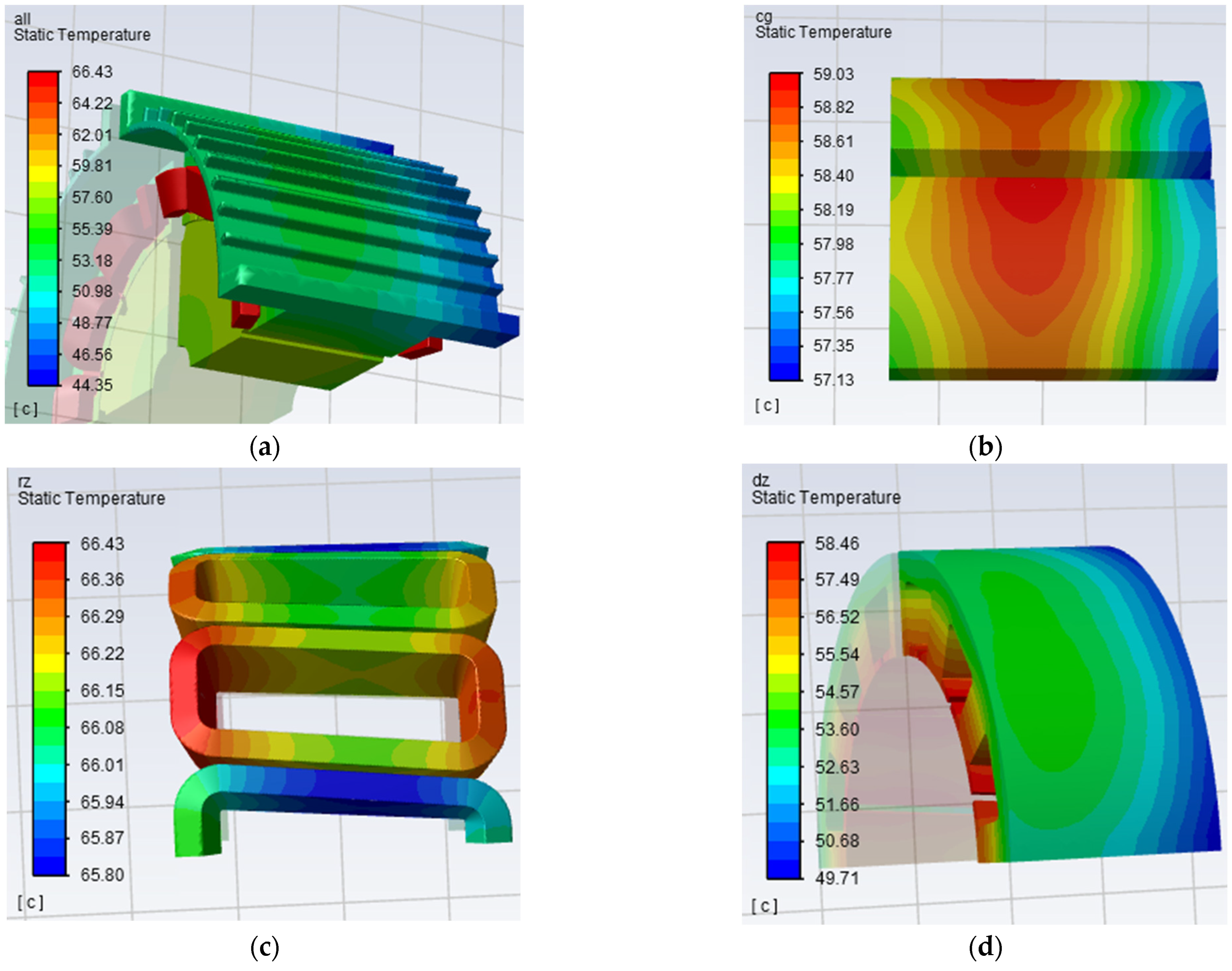
[20,21,22]. Figure 8 depicts the results of the EMTBC numerical calculation of the PMSM used to determine the temperature distribution field inside the motor.

To derive the specific temperature distribution rule within the motor, the temperatures of various components in Figure 8 were extracted, and the temperature gradients of the various components within the motor are depicted in Figure 9a. Because the high temperature of the permanent magnet (PM) causes demagnetization and the high insulation temperature of the winding causes a short-circuit defect, the temperature rise distribution of the PM and winding should be analyzed within a suitable range, as depicted in Figure 9b–d.

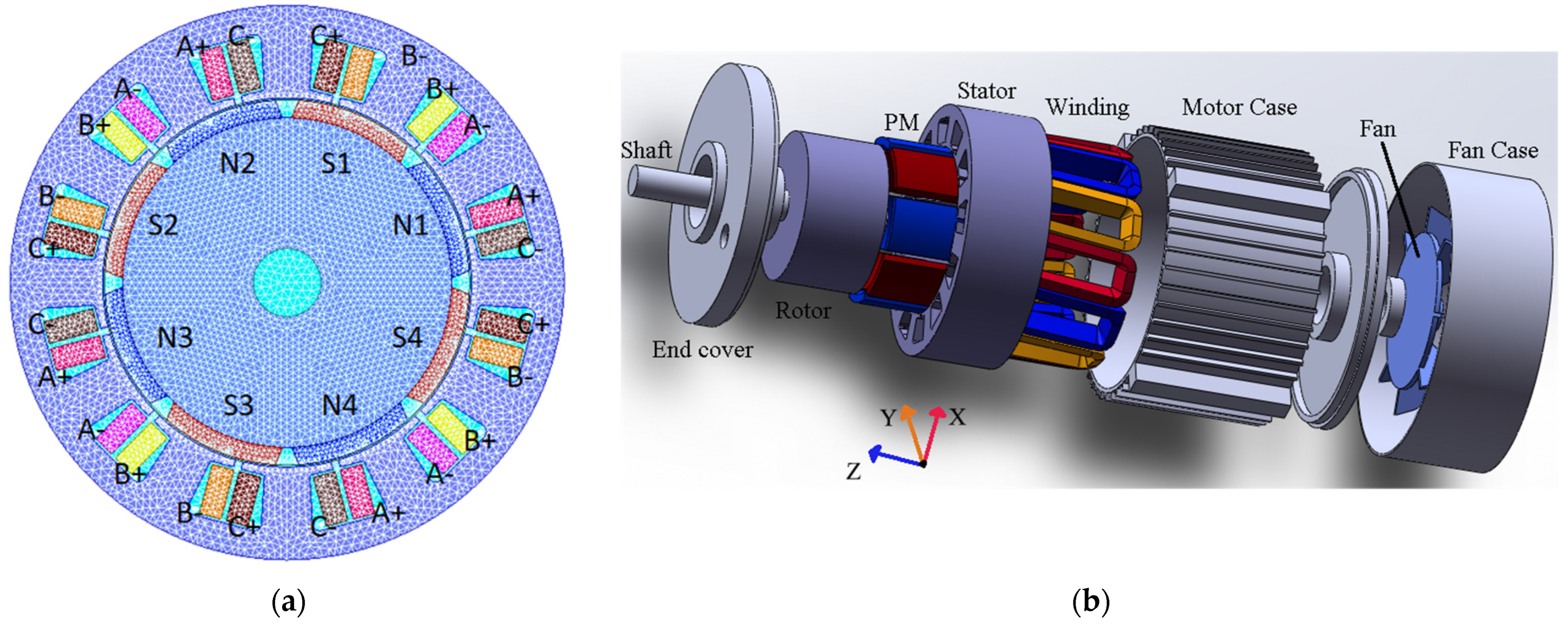
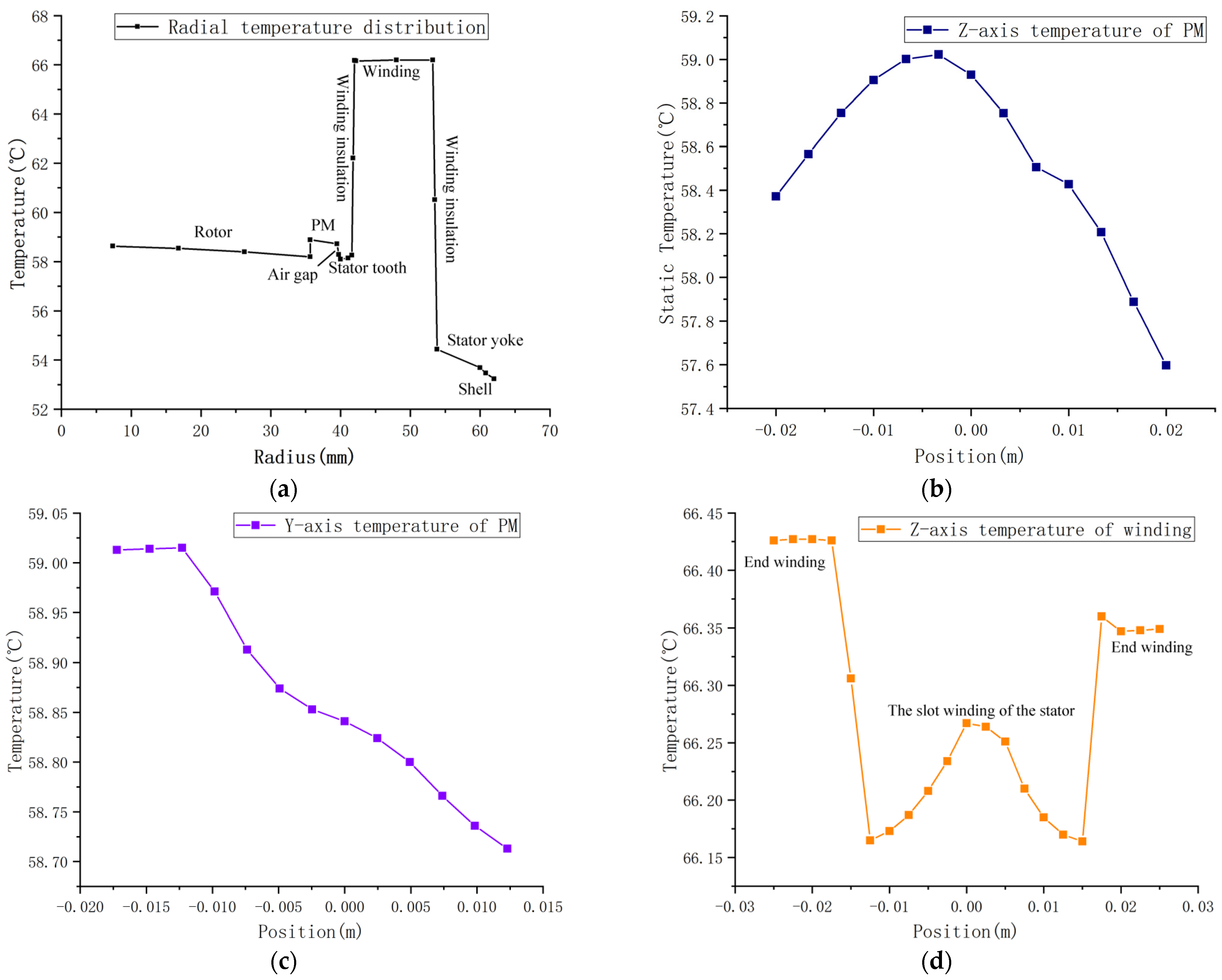
Figure 9a depicts the temperature gradient changes of the various motor components (where the orientation of the specific coordinate system is shown in Figure 2b). It indicates that the winding temperature is the highest, and the motor case temperature is the lowest. There are two protrusions: the temperature distribution of the PM and the temperature distribution of the winding. Since both the PM and the winding are heat sources, their temperatures are slightly higher than those of the surrounding contact portions. Figure 9b depicts the PM’s axial temperature distribution diagram. The PM temperature rise is higher in the middle and lower at both extremities, with the temperature on the right being lower than the temperature on the left. The following are the factors for this change:

• The axial middle section of the PM has poor heat dissipation;
• The motor is an axial air-cooled structure, and because the right side of the PM is near to the fan, its temperature is lower than that of the left side; Figure 9c is a diagram of the PM’s transverse temperature distribution.

The temperature near the middle border of the PM is the highest. The highest temperature of the PM is located in the axial middle of the PM and marginally near the edge of the middle of the two PMs, whereas the lowest temperature is located near the fan’s axial end. Figure 9d depicts the distribution of the winding’s axial temperature rise. Due to inadequate heat dissipation at the end of the winding, the temperature is the highest at both ends of the winding, and the temperature is the lowest near the fan and connected to the end of the winding.

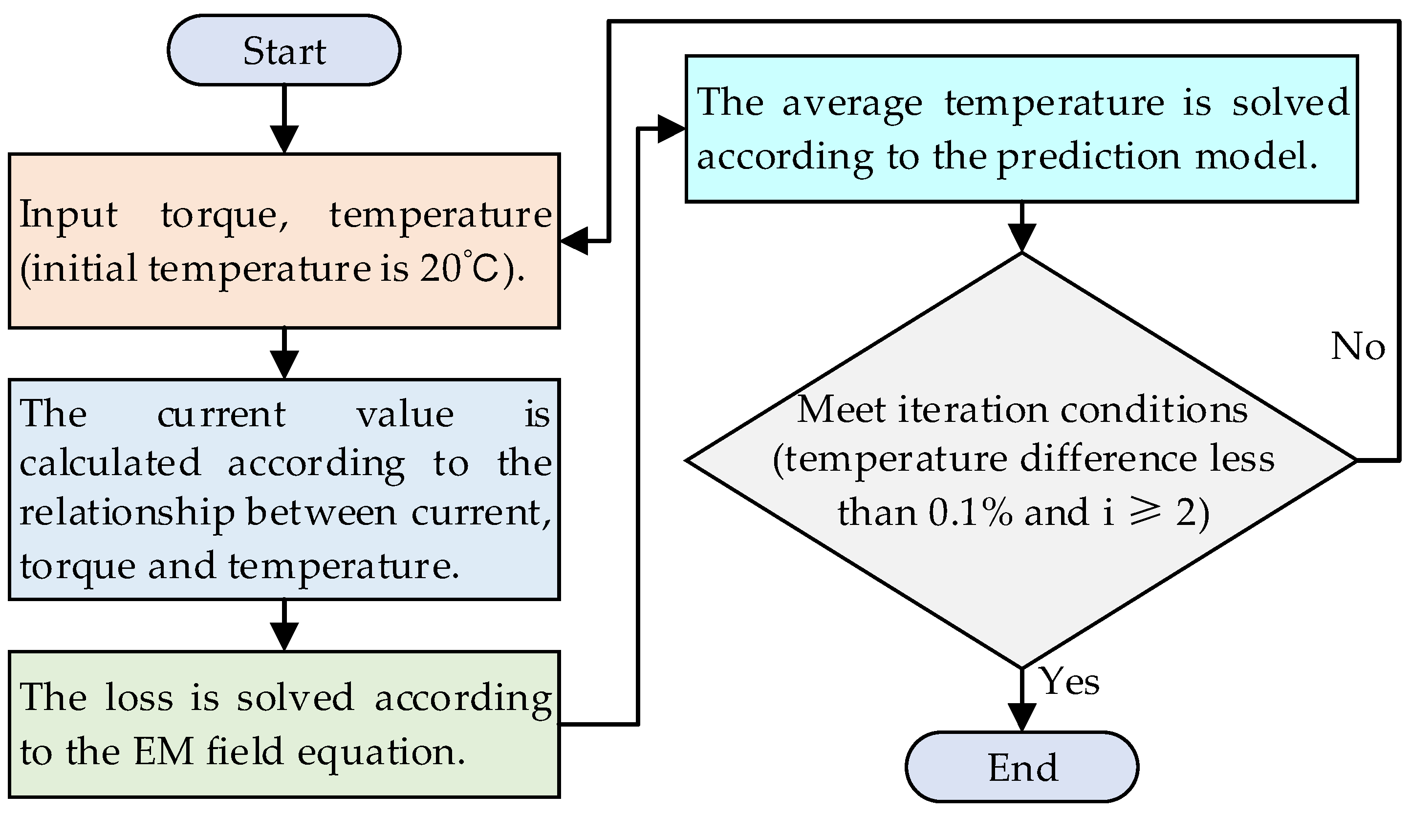
3.4.2. Establishment of Prediction of Regression Temperature Field Model

In the process of solving the internal temperature field of the PMSM using FEA, on the one hand, a large number of grids are required to simulate the real heat transfer process inside the PMSM; on the other hand, to account for the influence of temperature on the properties of EM materials, the temperature field and the EM field must constantly reverse iterate in order to achieve a certain level of calculation accuracy. Therefore, the traditional EMTBC method for solving temperature fields requires a great deal of calculation effort. To address this issue, we use the EM field loss data as the input to the temperature field and the highest and lowest winding and PM temperatures as the output. By constructing a high-precision proxy model to fit the mapping relationship between the input and output, it is possible to obtain a high-precision regression prediction model without an excessive amount of data samples, which significantly improves the computational efficiency of the temperature field.

To establish a high-precision regression prediction model, the sample point selection must satisfy the following criteria:

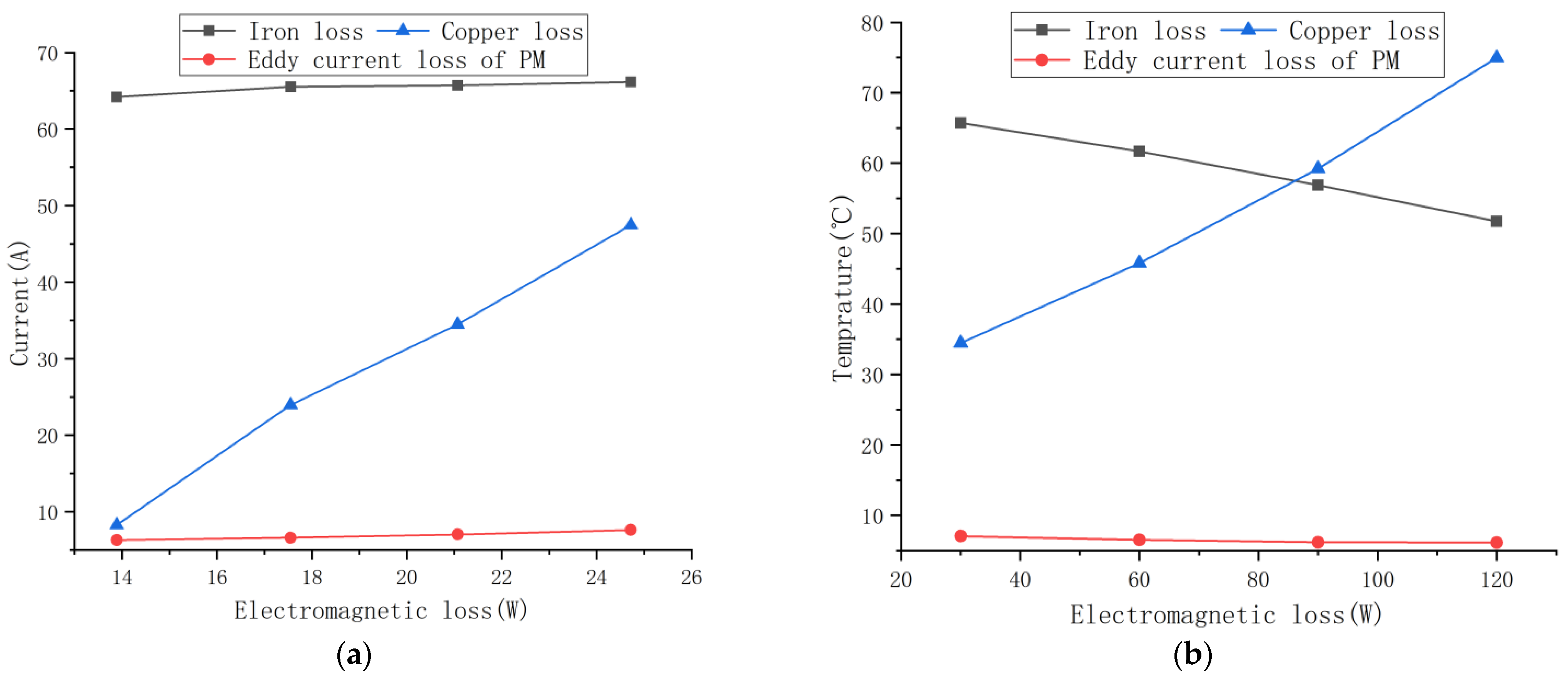
• The iron loss, eddy current loss of the PM loss, and copper loss input data have a certain correlation and cannot be combined at random.
• The PMSM load torque and operating temperature are two factors that influence the EM loss; consequently, the operating point should be evenly selected within the torque and temperature range of the motor.
• Since the solution of the temperature field is time-consuming, a regression prediction model with a higher accuracy should be obtained with fewer sample points than those of a traditional FEM.

In conclusion, based on the numerical calculation data of the EM field in Table 5, we selected 20 °C, 40 °C, 60 °C, 70 °C, 80 °C, 90 °C, 100 °C, and 110 °C and the rated EM torque, 1.25 times EM torque, 1.5 times EM torque, 1.75 times EM torque, and 2 times EM torque, and we conducted a numerical calculation of the temperature field at a total of 24 operating points.

This paper compares five common regression prediction models, which are as follows: (1) BP (Back Propagation), (2) SVR (support vector regression), (3) CNN (Convolutional Neural Network), (4) RF (Random Forest), and (5) LSTM (Long Short-Term Memory). First, the five regression prediction algorithms were used to build a proxy model for the input variable (loss) and the output target (temperature). Then, the accuracy of the proxy model was compared by calculating the evaluation index of the regression model. Finally, the one with the best evaluation index was selected as the regression prediction model in this paper. Commonly used regression model evaluation indexes include R² (the coefficient of determination), among which R² is the evaluation index that can best reflect the degree of fitting, and the closer the coefficient is to 1, the better the fitting degree. The calculation of this regression evaluation index can be expressed as follows [23]:

$$R^2=1-\frac{{\displaystyle {\sum }_{i=1}^n{(y_i-\stackrel{\wedge }{y_i})}^2}}{{\displaystyle {\sum }_{i=1}^n{(y_i-\overline{y_i})}^2}}$$

(15)

where n is the number of samples of the test set, y_i is the actual value of the test set sample, ŷ_i is the predicted value of the test set sample, and ӯ is the average value of the actual value of the test set sample. The specific evaluation indicators of each regression model after training are shown in

Table 7. Each agent model evaluation index.

Regression Prediction Method	Evaluating Indicator	Output Result
		Tmax-Winding (°C)	Tmin-Winding (°C)	Tmax-PM (°C)	Tmin-PM (°C)
BP	R2	0.996	0.996	0.994	0.996
SVR	R2	0.989	0.992	0.965	0.992
CNN	R2	0.944	0.954	0.960	0.922
RF	R2	0.731	0.762	0.727	0.823
LSTM	R2	0.996	0.986	0.998	0.991

.

In Table 6, it can be seen that both the BP neural network and LSTM models have a high level of prediction accuracy for the four output targets, but the BP neural network is superior. For each of the four output targets, the model developed by RF has a weak predictive accuracy. For all four output targets, the SVR- and CNN-constructed models provide more precise predictions. In conclusion, we propose the use of a BP neural network to build a regression prediction model.

Since the initial weight and threshold of a BP neural network are arbitrary, the network’s output is unstable [24]. If the initial weight and threshold are inadequate, the network will reach a local optimal state, resulting in a subpar prediction effect. To enhance the stability of the BP neural network’s prediction effect, we use a genetic algorithm to determine the optimal weight and threshold. 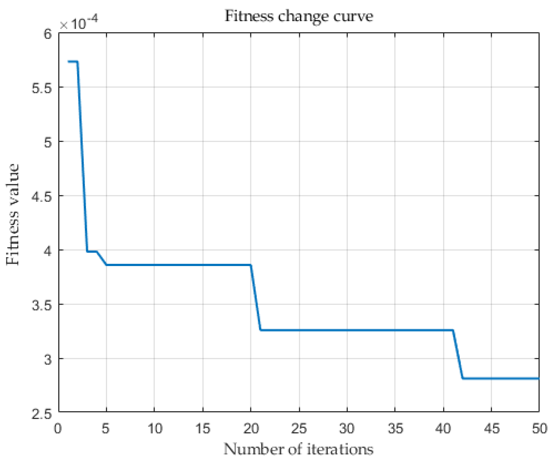Figure 10 depicts the iterative convergence process, while Table 6 depicts the final model effect.

Table 8. Model comparison before and after optimization.

Regression Prediction Method	Evaluating Indicator	Output Result
		Tmax-Winding (°C)	Tmin-Winding (°C)	Tmax-PM (°C)	Tmin-PM (°C)
BP	R2	0.996	0.996	0.994	0.996
GA-BP	R2	0.999	0.999	0.999	0.999

demonstrates that the genetic algorithm is used to determine the optimal weight and bias for BP, and that the enhanced GA-BP algorithm is more accurate and stable. Therefore, we propose the GA-BP model as the temperature field regression prediction model.

3.5. Bidirectional Coupling Solution Strategy Based on Reduced-Order Model

In Section 3.3 and 3.4, we establish the reduced-order solving models for the EM field and temperature, respectively. To simulate the iterative process of the EMTBC while taking into account the effect of the temperature field on EM materials, two reduced-order models are coupled and iterated to simulate the solution process of the EMTBC. The specific procedure is reported in the flow-chart in Figure 11.

This section is pre-programmed with two reduced-order models, so we only need to provide the initial load torque, and the model will solve the temperature distribution of the winding and PM automatically.

4. Results and Analysis

To verify the correctness of the efficient reduced-order EMTBC solution model and solution strategy proposed in this paper, the traditional EMTBC numerical temperature rise calculation, the traditional unidirectional EM thermal numerical temperature rise calculation, and the reduced-order EMTBC model temperature rise calculation were performed, and the three solution results were compared and analyzed as shown in

Table 9. Comparison of three calculation methods of temperature rise.

	Tmax-Winding (°C)	Tmin-Winding (°C)	Tmax-PM (°C)	Tmin-PM (°C)	Solution Time (Minute)
Traditional EMTBC numerical temperature rise calculation	61.85	61.27	56.17	54.75	160
Traditional unidirectional EM-thermal numer-ical temperature rise calculation	58.40	57.85	56.05	54.60	41
Difference (%)	5.56	5.58	0.21	0.27
Reduced-order EMTBC numerical temperature rise calculation	61.90	61.30	56.25	54.77	1
Difference (%)	0.081	0.049	0.14	0.036

.

Compared to the unidirectional EM-thermal numerical temperature rise calculation, the maximum temperature rise of the winding in the EMTBC numerical temperature rise calculation increases by 5.56 percent; the minimum temperature rise of the winding increases by 5.58 percent; and the maximum and minimum temperature rises of the PM increase by 0.21 percent and 0.27 percent, respectively. This also demonstrates that the EMTBC numerical temperature rise calculation is more precise. In the process of the EMTBC iteration, however, the solution time also increases significantly; the solution time is approximately 3 h, which is 2.9 times longer than the calculation time for the unidirectional EM-thermal numerical temperature rise. Moreover, by comparing the numerical temperature rise calculation results and solution time of our proposed reduced-order EMTBC model and the traditional EMTBC, it can be seen that there is a small difference in the numerical temperature rise calculation results between these two strategies, but the solving time is reduced by 159 times. Our proposed EMTBC dimensionality reduction model is therefore precise and effective.

5. Conclusions

This paper analyzes the effect of temperature on EM materials and concludes that temperature can reduce the EM performance of PMs in conventional electromagnetic FEA, resulting in a reduction in the EM torque. To keep the EM torque constant, the EMTBC injects an additional control current to enhance the precision of the results. However, the adopted EMTBC’s numerical calculation is time-consuming. To increase the computational efficiency, we propose a reduced-order EMTBC. The proposed model has been validated numerically, demonstrating high precision and efficiency. Nonetheless, the model proposed in this paper is intended to compute the temperature distribution under steady-state conditions. In future work, we will investigate and analyze the rise in temperature of the temperature field in real time under conditions of flux variation.

References

1. Zheng, J.Q.; Zhao, W.X.; Ji, J.H.; Li, H.T. Review on Design Methods of Low Harmonics of Fractional-slot Concentrated-windings Permanent-magnet Machine. Proc. CSEE 2020, 40, 272–280. [Google Scholar]
2. Cai, X.; Cheng, M.; Zhu, S.; Zhang, J. Thermal modeling of flux-switching permanent-magnet machines considering anisotropic conductivity and thermal contact resistance. IEEE Trans. Ind. Electron. 2016, 63, 3355–3365. [Google Scholar] [CrossRef]
3. Wang, Y.F.; Zhao, J.; Huang, J.B.; Wang, F. Impedence Parameters Analysis of Permanent Magnet Synchronous Motor under Inter-Turn Short Circuit Fault. Electr. Mach. Control. Appl. 2017, 44, 105–109. [Google Scholar]
4. Ding, S.Y.; Jiang, X.; Zhu, M.; Liu, W. Starting and steady temperature rise investigation for permanent magnet synchronous motor based on lumped-parameter thermal-network. Electr. Mach. Control 2020, 24, 143–150. [Google Scholar]
5. Mo, L.; Zhu, X.; Zhang, T.; Quan, L.; Wang, Y.; Huang, J. Temperature Rise Calculation of a Flux-Switching Permanent-Magnet Double-Rotor Machine Using Electromagnetic-Thermal Coupling Analysis. IEEE Trans. Magn. 2018, 54, 1–4. [Google Scholar] [CrossRef]
6. Yu, W.; Hua, W.; Qi, J.; Zhang, H.; Zhang, G.; Xiao, H.; Xu, S.; Ma, G. Coupled Magnetic Field-Thermal Network Analysis of Modular-Spoke-Type Permanent-Magnet Machine for Electric Motorcycle. IEEE Trans. Energy Convers. 2020, 99, 120–130. [Google Scholar] [CrossRef]
7. Wang, Z.P.; Wang, M.; Ding, S. Analysis on Correlated Sensitivity Factors of Temperature Rise for Surface Permanent Magnet Synchronous Motors. Proc. CSEE 2014, 34, 5888–5894. [Google Scholar]
8. Alberti, L.; Bianchi, N. A Coupled Thermal–Electromagnetic Analysis for a Rapid and Accurate Prediction of IM Performance. IEEE Trans. Ind. Electron. 2008, 55, 3575–3582. [Google Scholar] [CrossRef]
9. Ding, S.Y.; Shen, S.F.; Yang, Z.; Chen, S.X.; Dai, Y. Fluid-solid coupling simulation and performance analysis of high-speed permanent magnet synchronous motor. Electr. Mach. Control 2021, 25, 112–121. [Google Scholar]
10. Zhang, G.; Hua, W.; Cheng, M.; Zhang, B.; Guo, X. Coupled Magnetic-Thermal Fields Analysis of Water-Cooling Flux-Switching Permanent Magnet Motors by an Axially Segmented Model. IEEE Trans. Magn. 2017, 53, 1–4. [Google Scholar] [CrossRef]
11. Li, Y.; Zhang, C.; Xu, X. Bidirectional electromagnetic–thermal coupling analysis for permanent magnet traction motors under complex operating conditions. Trans. Can. Soc. Mech. Eng. 2022, 46, 541–560. [Google Scholar] [CrossRef]
12. Jia, M.; Hu, J.; Xiao, F.; Yang, Y.; Deng, C. Modeling and Analysis of Electromagnetic Field and Temperature Field of Permanent-Magnet Synchronous Motor for Automobiles. Electronics 2021, 10, 2173. [Google Scholar] [CrossRef]
13. Zhao, P.; Yu, Y. Analysis of Influence of Permanent Magnet Demagnetization on Motor Temperature Rise. J. Phys. Conf. Ser. 2022, 2395, 012022. [Google Scholar] [CrossRef]
14. Tang, R.Y. Modern Permanent Magnet Machines Theory and Design; China Machine Press: Beijing, China, 2015. [Google Scholar]
15. Qi, G. Research on Dual Three-Phase Permanent Magnet Brushless AC Motors Accounting for Cross-Coupling Magnetic Saturation. Ph.D. Thesis, Huazhong University of Science and Technology, Wuhan, China, 2010. [Google Scholar]
16. Zhong, Q.; Ma, H.Z.; Liang, W.M.; Chen, C. Preliminary Analysis of Demagnetization Fault Mathmatical Model for Permanent Magnet Synchronous Motor of Electric Vehicles. Micromotors 2013, 46, 9–12+18. [Google Scholar]
17. Zhang, Y.; McLoone, S.; Cao, W. Electromagnetic loss modeling and demagnetization analysis for high-speed permanent magnet machine. IEEE Trans. Magn. 2017, 54, 1–5. [Google Scholar] [CrossRef]
18. Liu, M.Y. Research on Iron Loss Model of High-Speed Permanent Magnet Motor Considering Multiphysics Factors. Master’s Thesis, Shenyang University of Technology, Shenyang, China, 2019. [Google Scholar]
19. Kuczmann, M.; Orosz, T. Temperature-Dependent Ferromagnetic Loss Approximation of an Induction Machine Stator Core Material Based on Laboratory Test Measurements. Energies 2023, 16, 1116. [Google Scholar] [CrossRef]
20. Shao, H. Research on Vibration and Temperature Rise of In-Wheel Motor For Electric Vehicle. Master’s Thesis, East China Jiaotong University, Nanchang, China, 2022. [Google Scholar]
21. Yao, H.Y. Simulation Study on Temperature Rise and Cooling Characteristics of Electric Vehicle In-Wheel Motor. Master’s Thesis, Jilin University, Changchun, China, 2019. [Google Scholar]
22. Wu, Y.H.; Liu, X.M. Research on Thermal Conductivity of Small Motor Windings. Micromotors 2015, 48, 27–29+37. [Google Scholar]
23. Yu, Y.; Pan, Y.; Chen, Q.; Hu, Y.; Gao, J.; Zhao, Z.; Niu, S.; Zhou, S. Multi-Objective Optimization Strategy for Permanent Magnet Synchronous Motor Based on Combined Surrogate Model and Optimization Algorithm. Energies 2023, 16, 1630. [Google Scholar] [CrossRef]
24. Li, W.H.; Niu, G.B.; Liu, Y.J. Hydraulic System Fault Diagnosis Based on Genetic Algorithm Optimized BP Neural Network. Mach. Tool Hydraul. 2023, 51, 159–164. [Google Scholar]
Figure 1. The steps of constructing a reduced-order solution model.
Actuators 12 00336 g001
Figure 2. Model of PMSM: (a) FEM; (b) Geometric Model.
Actuators 12 00336 g002
Figure 3. The influence of temperature on torque under the traditional model is solved.
Actuators 12 00336 g003
Figure 4. Temperature−torque−current fitting.
Actuators 12 00336 g004
Figure 5. Torque comparison based on the improved solution model.
Actuators 12 00336 g005
Figure 6. EM loss with load and temperature rise change relationship. (a) Effect of load on EM loss. (b) Effect of temperature on EM loss.
Actuators 12 00336 g006
Figure 7. The influence of load and temperature on EM loss: (a) the influence of load and temperature on iron loss; (b) the influence of load and temperature on eddy current loss of PM.
Actuators 12 00336 g007
Figure 8. The temperature distribution diagram of each part of the motor: (a) the temperature distribution diagram of the whole motor; (b) the temperature distribution diagram of the PM; (c) the temperature distribution diagram of the winding; (d) the temperature distribution diagram of the stator.
Actuators 12 00336 g008
Figure 9. Temperature gradients of various parts inside the motor; (a) radial temperature distribution of the motor; (b) axial temperature distribution of the PM; (c) lateral temperature distribution diagram of PM; (d) winding axial temperature distribution.
Actuators 12 00336 g009
Figure 10. Iterative process of genetic algorithm.
Actuators 12 00336 g010
Figure 11. Bidirectional coupling solution strategy based on reduced-order model.
Actuators 12 00336 g011