Balancing Control of an Absolute Pressure Piston Manometer Based on Fuzzy Linear Active Disturbance Rejection Control

Abstract

As an international standard pressure-measuring instrument, the absolute pressure piston manometer’s working medium is gas, so the actual working process will be affected by many internal uncertainties and external disturbances, leading to its long stability time and poor performance. In this paper, a fuzzy linear active disturbance rejection control strategy (FLADRC) for absolute pressure piston manometers is proposed to address these problems. First, the characteristics of the main components are analyzed according to the actual working principle of the system to establish a theoretical model of the controlled system. Second, the corresponding linear active disturbance rejection controller (LADRC) is designed according to the model. The principle of fuzzy control is introduced to adaptively adjust the controller parameters of the LADRC in real time, which improves the disadvantages of the LADRC parameters, which are difficult to rectify and have poor immunity to disturbances due to fixed parameters, and the stability of the control method is subsequently demonstrated. Finally, a simulation model is built in the Simulink environment in MATLAB, and three different pressure operating points are selected for the corresponding experiments to make a comparative analysis with Kp, PID, and LADRC. The results show that FLADRC enables the absolute pressure piston manometer to achieve better stability and greater immunity to disturbances. This also verifies the effectiveness and feasibility of the control strategy in practical engineering applications.

1. Introduction

In recent years, absolute pressure measurement technology has become one of the important symbols to measure the degree of industrial technology development of a country and is also an important evaluation indicator of industrial safety [1,2,3]. As an international standard pressure measurement instrument with high accuracy and stability, the absolute pressure piston manometer is based on the hydrostatic equilibrium principle and Pascal’s law for pressure measurement. As the working medium is a gas, the adiabatic manometer is subject to many nonlinear and time-varying factors, which results in relatively long stabilization times and unsatisfactory stability performance. Therefore, it is crucial to design a high-quality control system to address these issues.

Relatively few scholars at home and abroad have studied piston manometer balancing control methods, but for quadrotors [4,5], inverted pendulums [6,7,8], balancing vehicles [9,10], permanent-magnet synchronous motors [11,12], and other such similar balancing systems, there are many modern control algorithms currently applied, such as proportional-integral-derivative (PID) control [13,14,15], linear quadratic regulator control (LQR) [16,17], robust control [18,19], fuzzy control [20,21,22,23], adaptive control [24,25], sliding mode control [26,27,28], etc. Theoretically, the control methods applied to these equilibrium systems can also be applied to piston manometers. The authors in [29] introduced the relaxation factor into model predictive control (MPC), on which it was combined with hybrid PID control theory for applied control to improve the control performance of smart car path tracking across the board. The authors in [30] proposed a Udwadia–Kalaba theory-based adaptive robust control (UKBARC), applied to a permanent-magnet linear synchronous motor, which can both transform the control task with the desired trajectory as the desired constraint and deal effectively with system uncertainty. The authors in [31] proposed a sliding mode control method incorporating an adaptive strategy to achieve altitude tracking of a quadrotor under strong external disturbances, but the method requires high accuracy of the model and a relatively complex controller structure. The authors in [32] proposed an improved fuzzy logic controller based on Lyapunov’s criterion for the real-time oscillation and stability control of a coupled two-arm inverted pendulum, which improved the transient and steady-state response speed of the system to a certain extent, but the amount of operations in this controller is large and more difficult to implement in practical engineering. The authors in [33] combined the quantum particle swarm algorithm (QPSO) with the LQR control method. It used the former to search for the optimal values of the Q matrix as well as the weighting coefficients in the controller, improving the overall control performance of the balancing vehicle, but the time for the algorithm to perform the optimal search still needs to be improved.

Active disturbance rejection control (ADRC) is an “observation + compensation” nonlinear control method proposed by Professor Jingqing Han et al. [34] to preserve the advantages of PID and overcome its shortcomings. However, the internal parameters are too many, and the rectification process is tedious. Gao [35] then introduced the concepts of linearization and bandwidth based on the advantages of active disturbance suppression techniques and proposed linear active disturbance rejection control (LADRC) for the first time, making the controller parameters more intuitive and simpler to rectify. In addition, to further improve the control performance of LADRC, many researchers have made further improvements. An improved third-order LADRC controller was proposed by the authors in [36], introducing the total disturbance differential signal in the LESO and applying a series of first-order inertial links, which improves the system’s ability to suppress high-frequency noise. The authors in [37] combined robust sliding mode control (SMC) theory with LADRC control to overcome the bandwidth limitation of LADRC itself and improve the control accuracy for the system. The authors in [38] proposed an improved linear active disturbance suppression control (MLADC) method to compensate the system model into a linear state observer (LESO) to improve its observation accuracy, reduce its state error and enhance the robustness of the system.

However, it is easy to see that most improvements have a common limitation, namely that the controller parameters can only be adjusted manually by trial and error, which is complex and time-consuming, and the fixed parameters also lead to a less robust system, which cannot be applied to specific practical engineering problems. As a nonlinear system, absolute pressure piston manometers cannot be modeled with absolute accuracy. Moreover, when implementing control, uncertainties within the system and external disturbances are inevitable, which can reduce the efficiency of the system [39], and the stability performance of the system needs to be improved. Fuzzy control is considered to be a control scheme to improve the robustness and adaptability of the system and has been widely used in industry. It can dynamically adjust the parameters of the controller according to the output of the system, thus enabling the controller to track the input signal faster. Therefore, to improve the anti-disturbance capability of the controlled system and make it achieve equilibrium quickly and stably, this paper proposes a FLADRC-based equilibrium control strategy for the adiabatic piston manometer, which introduces the idea of fuzzy control for adaptive parameter adjustment based on LADRC. The feasibility and effectiveness of the control scheme are verified by simulations in MATLAB.

The other sections of the article are organized as follows: In Section 2, the theoretical modeling of the adiabatic piston manometer is presented. In Section 3, the specific design and stability analysis of the FLADRC controller is carried out for the controlled system model. In Section 4, the simulation results of the four control schemes, FLADRC, LADRC, PID, and Kp, are compared and analyzed to verify the performance advantages of the proposed control scheme. Finally, the summary of the research work in this paper is discussed in Section 5.

2. Theoretical Modeling of an Absolute Pressure Piston Manometer

2.1. The Working Principle of the Absolute Pressure Piston Manometer

The mechanical structure of the absolute pressure piston manometer as a nonlinear time-varying system is shown in Figure 1. Before the system starts to work, the corresponding weights are automatically configured according to the measured pressure. The pure gas in the cylinder, which is the working medium for pressurizing the system, is first added quickly to the originally vacuumed piston cylinder through the inlet valve until the weights and the piston is jacked up. Immediately afterward, the piston is subjected to constant changes in height due to the pressure in the piston cylinder and other uncertainties. The gas flow from the inlet and outlet valves is then adjusted in turn according to the actual situation so that the piston is finally stabilized at the preset height. At this point, the weights and piston are then mechanically balanced as a whole, thus completing the measurement and calibration of the pressure.

Based on the above working principle, it can be seen that the most important part of the system is the piston, followed by the electromagnetic switching valve. Therefore, to build a theoretical model for an absolute pressure piston manometer, it is necessary to start with these two parts and carry out the corresponding characteristic analysis.

2.2. Kinetic Analysis of the Weight Combination Section

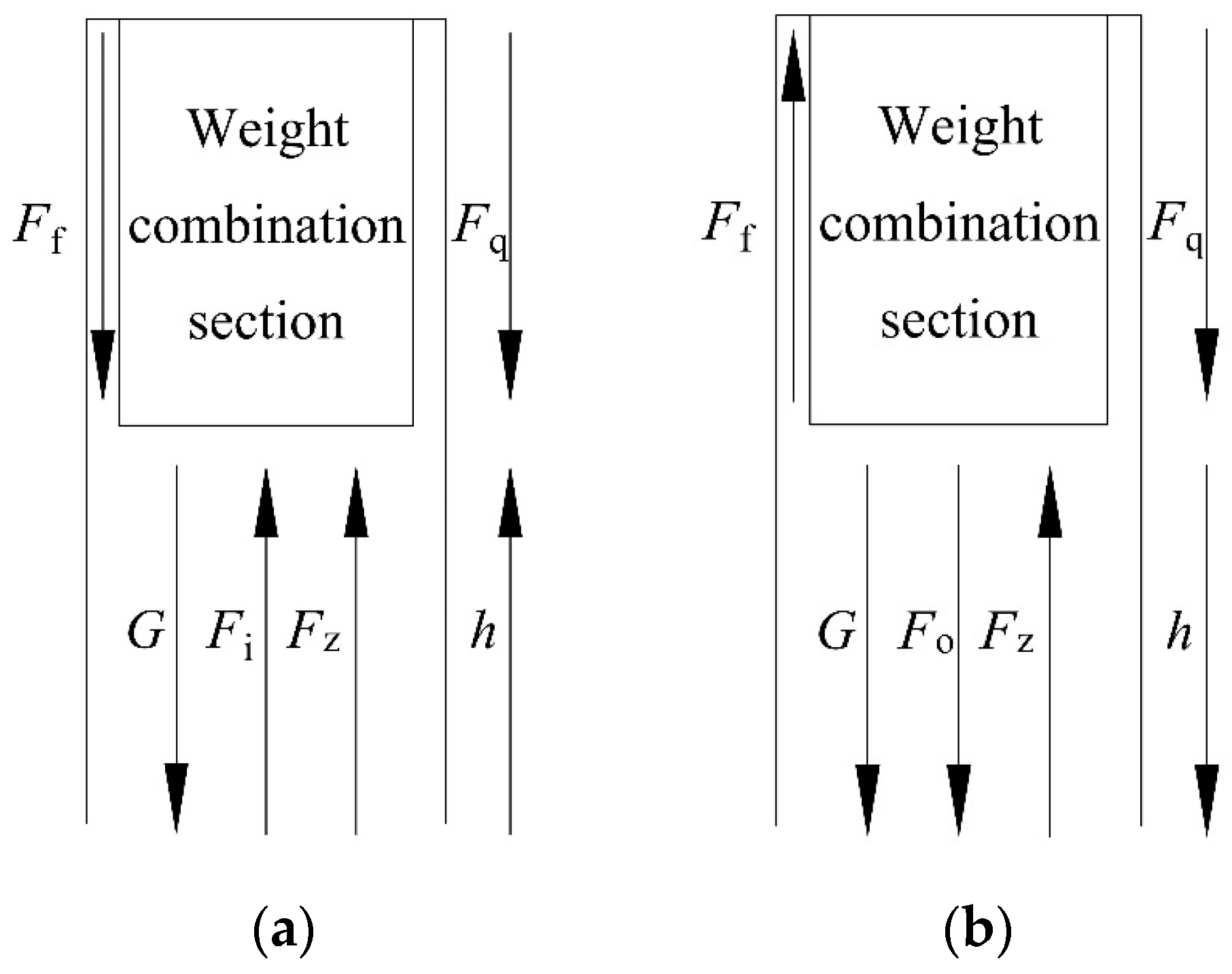
Throughout the actual working of the system, the weight, the weight plate, and the check piston can be seen as a whole, collectively referred to as the weight combination part. In the force analysis of this whole, the weight combination is subjected to its own gravity G, the pressure F_v resulting from the change in mass of the gas in the piston cylinder (F_i and F_o depending on the inlet and outlet processes), the resistance F_f of the gas preventing the change in the height of the piston, the pressure F_q lost by the gas leakage and the elastic force F_z resulting from the compression of the gas in the cylinder. Take vertical upwards as the positive direction.

As can be seen from Figure 2, the weight combination part is subjected to different magnitudes and directions of partial forces in the two different working processes of rising and falling, which have to be analyzed separately, thus listing the kinetic equilibrium equations of the weight combination part in in the two states of motion according to Newton’s second law, as in Equation (1).

$$\left\{\begin{array}{l}{F}_i-G-F_f-F_q+F_z=m_w\ddot{h}\\ -F_o-G+F_f-F_q+F_z=-m_w\ddot{h}\end{array}\right.$$

(1)

where m_w is the total mass of the combined portion of weights and h is the real-time height at which the piston rises. The process by which the gas is compressed and thus expands is similar to that of a spring, and the process by which the gas in the gap in the side of the piston prevents the piston from rising is similar to that of a damping system, so the resistance F_f can be calculated using Equation (2) and the elastic force F_z can be calculated using Equation (3).

$$F_f=c\dot{h}$$

(2)

$$F_z=kx$$

(3)

where c is the dynamic viscosity of the gas medium, k is the coefficient of elasticity after the compression and expansion of the gas in the cylinder is equivalent to a spring system, and x is the actual compression of the gas in the cylinder. Taking the process of gas intake as an example, the process of calculating the elasticity coefficient after equivalence is as follows: the instantaneous moment when the intake valve has been fed once is analyzed and calculated, at which time the gas volume is compressed and reduced by ΔV, and the pressure is increased by ΔP. According to the basic principles of elasticity, there is Equation (4).

$$\Delta P=-E(\Delta V/V_0)$$

(4)

where V₀ is the cylinder volume corresponding to the primary gas intake and is a fixed value that can be calculated from the flow rate of the intake valve, and E is the modulus of elasticity of the gas media. At this point, according to the calculation Equation of the elastic force generated by the compression of the gas (5), the calculation Equation of the piston cylinder volume (6), and Equation (3), the calculation formula of the elasticity coefficient (7) can be deduced.

$$F=-\Delta P·A=E(\Delta V/V_0)A$$

(5)

$$\Delta V=x·A$$

(6)

$$k=(E{A}^2)/V_0$$

(7)

The relationship between the gas compression and the actual rise of the piston is x = h_n − h, where h_n is the ideal height of the piston rise after n gas inlets without taking into account the gas compression, which needs to be determined according to the actual mass of the intake gas.

In summary, the elastic force F_z in Equation (1) can be expressed by Equation (8).

$$F_z=(E{A}^2)(h_n-h)/V_0$$

(8)

The pressure F_v in Equation (1) is the driving force for the entire combined part of the piston and can be calculated using the actual gas state Equation (9) as well as the pressure Equation (10) in the closed vessel together.

$$P{V}_2=ZnRT$$

(9)

$$F_v=P·A=(ZnRTA)/V_2$$

(10)

where R is the molar constant of the gas media, T is the thermodynamic temperature, Z is the compression coefficient of the gas media, P is the real-time pressure in the piston cylinder, n is the number of moles of gas in the cylinder, and the formula is n = m_t/M. Taking the inlet process as an example, m_t is the mass of gas entering the piston cylinder through the inlet valve, and M is the molar mass of the gas media. V₂ is the volume in the cylinder after the piston has risen to an expected height and is a fixed value.

2.3. Flow Analysis of Switching Valves

Solenoid switching valves, as actuators in the controlled system, can be divided according to their actual function into inlet and outlet valves, the most important characteristic of which is the real-time gas flow through the valve body. The switching valve can be seen as a throttle plate with a regularly varying orifice diameter, each switch corresponding to a maximum opening and a zero opening. The equation for the gas mass flow rate of the solenoid switch valve is obtained as follows [40].

$$m_{in}=C_d{A}_1\sqrt{2\Delta P_1\rho }$$

(11)

$$m_{out}=C_d{A}_1\sqrt{2\Delta P_2\rho }$$

(12)

where m_in is the gas inlet mass of the single switch of the inlet valve body, m_out is the outlet mass of the single switch of the gas outlet valve body, C_d is the flow coefficient, A₁ is the flow area of the valve opening, ΔP₁ is the pressure difference between the left and right of the inlet valve body, ΔP₂ is the pressure difference between the left and right of the inlet valve body, and ρ is the density of the gas medium in the gas cylinder.

Remark 1. 

The nonlinear factors in the controlled system are linearized, assuming that the control command u and the actual mass flow rate in and out of the valve are equal, i.e., the actuator can fully satisfy the control force command. However, in practical engineering, due to the limitations of the physical mechanism, the frequency of the number of times the solenoid valve can be switched on and off is limited, and therefore the inlet and outlet flow rates per unit of time are also bounded, so they are converted into an inequality form constraint, which is reflected in Equation (13).

$$\left\{\begin{array}{l}{m}_{1t}\le m_1=15m_{in} Gas in\\ m_{2t}\le m_2=15m_{out} Gas out\end{array}\right.$$

(13)

2.4. Analytical Correction of Other Uncertainties

In the process of theoretical modeling, the internal uncertainties of the controlled system should be considered to be comprehensively as possible to obtain a higher accuracy of the system modeling. Compensating these factors into the controller can also, to some extent, improve the control performance of the system [41].

2.4.1. Analytical Correction of Piston Effective Area

During the operation of the manometer, as the temperature, as well as the pressure, continues to rise, the piston will produce a certain elastic deformation, and its effective working area will then change. Assuming that the influence of external factors is not taken into account, the effective area of the piston can be calculated by Equation (14).

$$A=\pi r^2+\pi r\delta$$

(14)

where r is the piston rod radius, and δ is the clearance between the piston rod and the piston cylinder.

However, in the actual operation of the manometer, the effective area of the piston is affected by the temperature and pressure when the effective area of the piston is calculated by Equation (15):

$$A_0=A\left[1+\left({\alpha }_c+{\alpha }_e\right)\left(\theta -20\right)\right]\left(1+\lambda P\right)$$

(15)

where a_c is the thermal deformation coefficient of the piston cylinder, a_e is the thermal deformation coefficient of the piston, θ is the temperature of the piston system during actual operation, λ is the elastic deformation coefficient of the piston at the bottom of the piston, and P is the working pressure at the bottom of the piston rod.

2.4.2. Analytical Correction of Gas Leakage Volumes

During the operation of the system, there is a gap between the checking piston and the cylinder. As the system pressure rises, some of the gas media will leak through the gap, resulting in pressure loss within the piston cylinder and affecting the rise height of the piston. According to engineering thermodynamics, knowledge can be known between the piston rod and the piston cylinder, in which the concentric annular gap flow can be approximated as a flat slit flow [42]; at this time, the formation of differential pressure flow leakage formula for Equation (16):

$$Q_t=\frac{\pi d{\delta }^3\Delta P_0}{12\mu L}$$

(16)

where Q_t is the real-time gas leakage, d is the diameter of the checking piston, ΔP₀ the pressure difference between the two ends of the piston gap leakage surface, L is the length of the flow path, and δ the width of the annular gap.

The value of the pressure loss due to gas leakage can be calculated according to Poiseuille’s law, as shown in Equation (17).

$$F_q=\frac{8\mu L{Q}_t}{\pi r^4}$$

(17)

2.5. Establishment of the Differential Equilibrium Equations of the System

Combined with the characterization of the two core components of the system and the analytical correction of some of the uncertainties inherent in the actual operation of the system, this leads to a specific mathematical theoretical model of the adiabatic piston manometer, i.e., the differential equilibrium equations of the system. Taking the kinetic equilibrium Equation (1) as the main body, Equations (2), (8), (10), (12), (13), (15) and (17) are substituted into it to supplement it, and finally, the overall differential equilibrium Equation (18) of the system is obtained.

$$\left\{\begin{array}{l}\frac{m_{1t}ZRT{A}_0}{M{V}_2}-a-m_{w}g-c\dot{h}-\frac{8\mu L{Q}_t}{\pi r^4}+(E{A}_0{}^2)(\frac{m_{1t}}{\rho A_0}-h)/V_0=m_w\ddot{h}\\ b-\frac{m_{2t}ZRT{A}_0}{M{V}_2}-m_{w}g+c\dot{h}-\frac{8\mu L{Q}_t}{\pi r^4}+(E{A}_0{}^2)(h-\frac{m_{1t}}{\rho A_0})/V_0=-m_w\ddot{h}\end{array}\right.$$

(18)

where m_1t is the real-time inlet mass flow rate of the inlet valve, and m_2t is the real-time inlet mass flow rate of the outlet valve, both of which are input signals to the system and the output signal is the real-time rise height h of the piston, the others are fixed system parameters.

According to the actual working principle of the system, it can be determined that the real-time height of the piston needs to be compared with the set value when realizing the system control, and based on the result, the switching of the working state equation is selected. Equation (18) from top to bottom is the differential balance equation for the inlet and outlet states of the system, respectively. Each switch is made based on the previous working state, so we add the outgoing gas factor a and incoming gas factor b to Equation (18). a is the effect of the total outgoing air volume on the driving pressure before the system is switched to the inlet state, and b is the effect of the total air intake on the driving pressure before the system switches to the outgoing air state, both of which are constants when in the differential equations of their respective states.

To make the differential equilibrium equation of the system more intuitive and concise and to facilitate the design of the corresponding controller, the author rearranges and simplifies Equation (18) to obtain Equation (19).

$$\begin{array}{c}\left\{\begin{array}{l}{K}_1{m}_{1t}=K_2\ddot{h}+K_3\dot{h}+K_{4}h+K_{51}\\ K_1{m}_{2t}=K_2\ddot{h}+K_3\dot{h}+K_{4}h+K_{52}\end{array}\right.\\ K_1=\frac{ZRT{A}_0}{M{V}_2}+\frac{E{A}_0}{\rho V_0}\\ K_2=m_w\\ K_3=c\\ K_4=\frac{E{A}_0{}^2}{V_0}\\ K_{51}=a+m_{w}g+\frac{8\mu L{Q}_t}{\pi r^4}\\ K_{52}=b-m_{w}g-\frac{8\mu L{Q}_t}{\pi r^4}\end{array}$$

(19)

As can be seen from Equation (19), the equilibrium equations for both the inlet and outlet conditions are very similar, with the same constant coefficients for all terms except for the constant term. In the design and simulation of the controller, the constant term only affects the initial point of the system and does not affect the control performance of the system or the simulation results, so the constant term can be ignored. To make the controller structure more simple and clear, combined with Remark 1, the two separate actuator outputs can be regarded as a positive and negative control quantity, with a positive value representing the inlet valve working alone and a negative value representing the outlet valve working alone, so that the final differential equilibrium equation of the system becomes Equation (20).

$$\left\{\begin{array}{l}{K}_1{m}_t=K_2\ddot{h}+K_3\dot{h}+K_{4}h\\ m_1<m_t<m_2\end{array}\right.$$

(20)

3. Design of the Controller

As the absolute pressure piston manometer is subject to many internal uncertainties during actual operation, the LADRC controller can effectively estimate the internal and external disturbances of the system in real time while compensating accordingly. The LADRC was therefore chosen for balanced control of the system, but given the fixed parameters, the controller lacked adaptability, poor control performance, and weak resistance to interference. Therefore, this section introduces the idea of fuzzy control to improve the traditional LADRC method and proposes a fuzzy linear self-anti-disturbance-based absolute pressure piston manometer controller. The details are as follows. Numbered lists can be added as follows:

3.1. Design of the LADRC

3.1.1. Structure of the LADRC

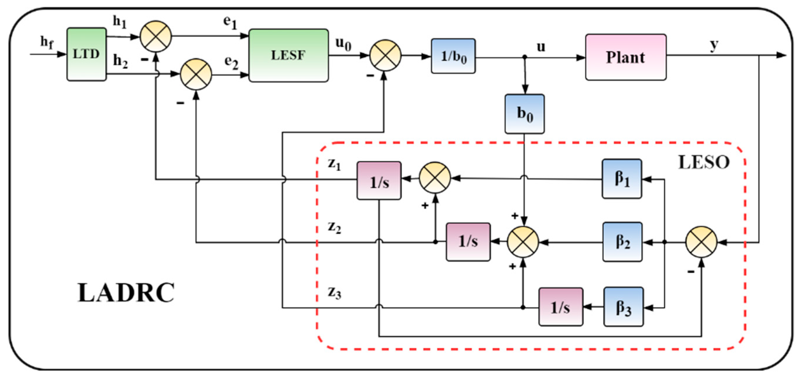
LADRC, as a modern control method, enables the system to maintain good dynamics and a steady state under disturbances such as noise, load disturbances, and changes in the mathematical model and process parameters. In this subsection, the corresponding LADRC controller is designed based on the theoretical model of the system developed, as shown in Figure 3. The components include a linear differential tracker (LTD), a linearly expansive state observer (LESO), and a linear error feedback control rate (LESF), with the specific design of each part as follows.

3.1.2. Design of the LTD

The LTD arranges the transition process for the input height signal and selects the appropriate parameters, which can make the output fast and overshoot-free, eliminating the contradiction between the amount of overshoot and the speed of control and also preventing sudden changes in the input signal, obtaining the differential signal and improving the robustness of the control system. The LTD design for the piston’s ideal height is as follows:

$$\left\{\begin{array}{l}{\dot{h}}_1=h_2\\ {\dot{h}}_2=-2r^2(h_1-h_f)-2r{h}_2\end{array}\right.$$

(21)

where: h_f is the given value input value, h₁ is the softened height given value, and h₂ is the differential signal of h₁, which are used later in the design of the state error feedback controller. r is the tracking speed factor.

3.1.3. Design of the LESO

LESO is the central part of the self-anti-disturbance control, which is capable of both tracking and estimating the height of the piston rise in the manometer and its differential signal in finite time when the system has an input signal, and estimating the total disturbance to the system in real time [43]. It can also be seen from Equation (20) that the adiabatic piston manometer is a second-order single-input, single-output system and, according to the operating principle of the LADRC, the system equation can be expressed as:

$$\left\{\begin{array}{l}\ddot{h}(t)=f(h(t),\dot{h}(t),t)+b_{0}u(t)\\ y(t)=h(t)\end{array}\right.$$

(22)

where u(t) is the input variable; y(t) is the output variable; b₀ is the system gain; $f(h\left(t\right),\dot{h}\left(t\right),t)$ is the generalized perturbation of the system, abbreviated as f() for neatness, expanding f() to a new state variable. The resulting state variables have been chosen as follows.

$$\left\{\begin{array}{l}{x}_1(t)=y(t)=h\\ x_2(t)=\dot{y}(t)=\dot{h}\\ x_3(t)=f()\end{array}\right.$$

(23)

The system equations can then be expressed in the form of an equation of state as follows:

$$\left\{\begin{array}{l}{\dot{x}}_1=x_2\\ {\dot{x}}_2=x_3+bu\\ {\dot{x}}_3=\dot{f}\end{array}\right.\Rightarrow \left\{\begin{array}{l}\dot{x}=Ax+Bu+C\dot{f}\hfill \\ y=Dx\hfill \end{array}\right.$$

(24)

Of which $x={\left[\begin{array}{ccc}{x}_1& x_2& x_3\end{array}\right]}^T$, $A=\left[\begin{array}{ccc}0& 1& 0\\ 0& 0& 1\\ 0& 0& 0\end{array}\right]$, $B={\left[\begin{array}{ccc}0& b& 0\end{array}\right]}^T$, $C={\left[\begin{array}{ccc}0& 1& 0\end{array}\right]}^T$, $D=\left[\begin{array}{ccc}1& 0& 0\end{array}\right]$.

As a result, the corresponding LESO is designed as:

$$\{\begin{array}{ll}\hfill \dot{z}& =Az+Bu+\beta (y-\hat{y})\hfill \\ & =Az+Bu+\beta (y-Dz)\hfill \\ \\ \hat{y}\hfill & =Dz\hfill \\ \end{array}\Rightarrow \left\{\begin{array}{l}{\dot{z}}_1={\mathrm{z}}_2+{\beta }_1(y-{\mathrm{z}}_1)\\ {\dot{z}}_2={\mathrm{z}}_3+{\beta }_2(y-{\mathrm{z}}_1)+b_{0}u\\ {\dot{z}}_3={\beta }_3(y-{\mathrm{z}}_1)\end{array}\right.$$

(25)

where $z_i={\left[\begin{array}{ccc}{z}_1& z_2& z_3\end{array}\right]}^T$ is the matrix of observer output estimates, z₁ tracks the estimated height of the piston rise in the actual manometer, z₂ tracks the estimated speed of the piston rise, and z₃ is the estimate of the total perturbation f(); and ${\beta }_i={\left[\begin{array}{ccc}{\beta }_1& {\beta }_2& {\beta }_3\end{array}\right]}^T$ is the observer gain matrix. The bandwidth method was proposed to rectify the observer gain parameters [35], let the bandwidth of the observer be ω₀ and try to configure all the eigenvalues of the observer as −ω₀, i.e.,

$${\lambda }_0(s)=\left|SI-(A-\beta D)\right|=s^3+{\beta }_1{s}^2+{\beta }_{2}s+{\beta }_3={(s+{\omega }_0)}^3$$

(26)

At this point, the above equation satisfies the Hurwitz condition, and β₁, β₂, and β₃ all become functions with respect to ω₀, i.e.,

$$\left\{\begin{array}{l}{\beta }_1=3{\omega }_0\\ {\beta }_2=3{\omega }_0^2\\ {\beta }_3={\omega }_0^3\end{array}\right.$$

(27)

Remark 2. 

Observability judgments are made according to Equation (24). Let N = (D, DA)^T, since rank(N) = 3, from which it follows that the expansion system is fully observable.

3.1.4. Design of the LESF

The LESF takes the error between the TD’s output and the estimated system state by linearly combining them to form the initial control quantity and then adding compensation for the total disturbance estimated by the LESO to obtain the final control quantity as in Equation (28).

$$\left\{\begin{array}{l}{e}_1=h_1-z_{i1}\\ e_2=h_2-z_{i2}\\ u_0=k_1{e}_1+k_2{e}_2\\ u=(u_0-z_3)/b_0\end{array}\right.$$

(28)

where: e₁ is the error between the LESO’s estimate of the piston rise height, and the preset height input value, e₂ is the error between the LESO’s estimate of the piston rise speed and the differential signal of the input value; k₁ and k₂ are the feedback control parameters; u₀ is the state error feedback control quantity. For the consideration of the dynamic performance of the LESF link, the same choice of the pole configuration method is used to rectify the two feedback control parameters so that the closed-loop transfer function has a pole of −ω_c and is solved as.

$$\left\{\begin{array}{l}{k}_1={\omega }_c^2\\ k_2=2{\omega }_c\end{array}\right.$$

(29)

where ω_c is the controller bandwidth, for most common engineering objects, ω_c and ω₀ have a multiplicative relationship, i.e., ω₀ = (3~5)ω_c [44], in this paper ω₀ = 4ω_c is taken.

3.2. Design of the FLADRC

3.2.1. Structure of the FLADRC

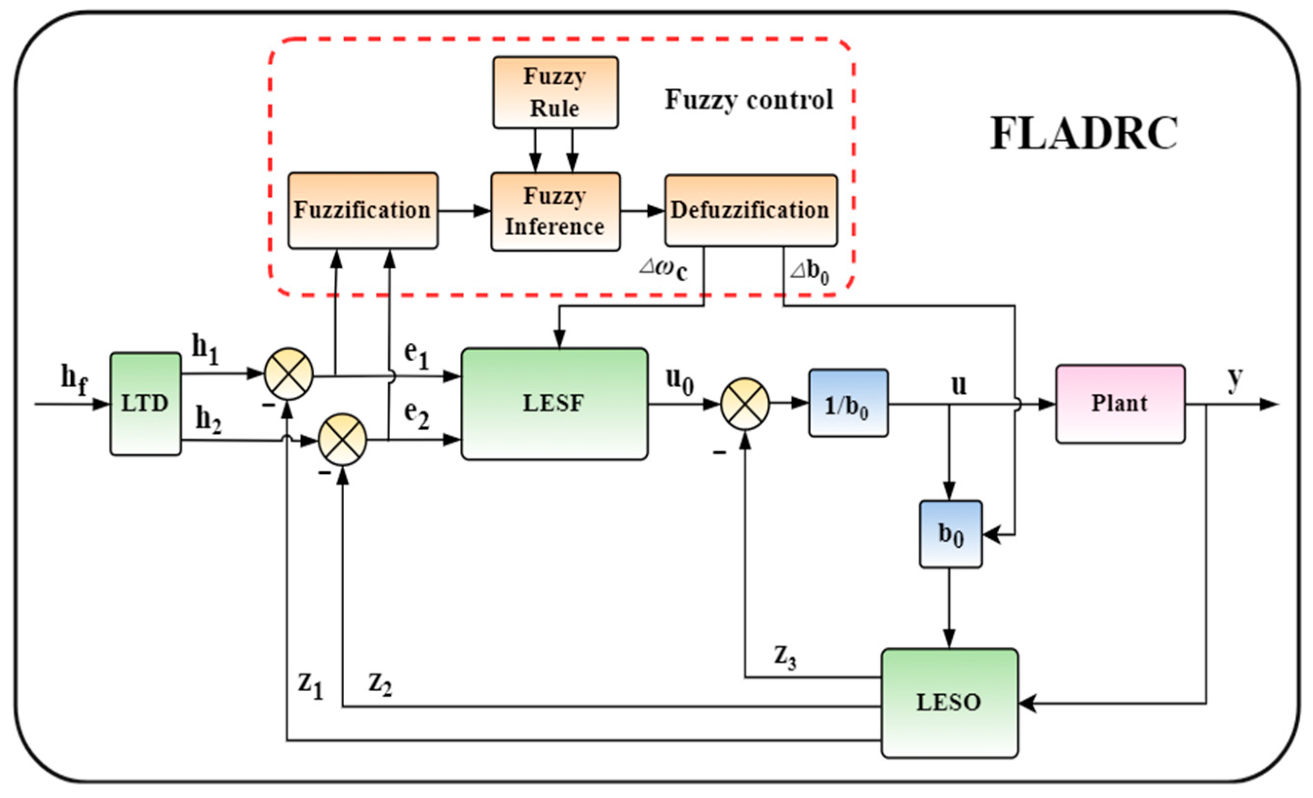
The application of LADRC to the control of an equilibrium system does reduce the pressure on the adjustment of the control parameters, but the fixed parameters do affect the stability and adaptability of the system to internal and external disturbances. In this paper, fuzzy control is introduced to adjust the parameters Δω_c and Δb₀ in the LADRC online and in real time so that the two parameters meet the requirements of the errors e₁ and e₂ at different times, thus improving the system’s immunity to disturbances and stability performance. The specific control structure of the fuzzy LADRC is shown in Figure 4.

3.2.2. Design of the Fuzzy Controller

The overall process of fuzzy control can be divided into four modules, namely fuzzy quantization processing, which converts precise inputs into fuzzy linguistic values; establishing fuzzy control rules, which establishes specific fuzzy control rules based on expert experience and the actual equilibrium requirements of a specific system; fuzzy inference, which inferred the output values of fuzzy control based on the input–output relationships embedded in the fuzzy inputs and rule base; and defuzzification processing The output values are defuzzified to obtain the actual parameters. The detailed design is as follows.

The fuzzy input linguistic variables selected in this paper are the error e₁ between h₁ and z₁ and its corresponding rate of change of deviation e₂, and the theoretical domains of both are selected to be [−2 × 10⁻³, 2 × 10⁻³] and [−1 × 10⁻³, 1 × 10⁻³], respectively. The outputs of the fuzzy controller are chosen to be Δω_c and Δb₀, where the theoretical domains of the two are assumed to be Range1 and Range2, respectively, the specific values of which are shown in the subsection on Experimental Parameter Settings later on. Seven subsets of the fuzzy language are defined on the respective theoretical domains of the inputs and outputs: {negative big (NB), negative medium (PM), negative small (NS), zero (ZO), positive small (PS), positive medium (NM), positive big (PB)}. Gaussian-type affiliation functions with smooth transitions are chosen for the inputs and high-sensitivity triangular affiliation functions for the outputs.

The traditional Mamdani inference method [45] was used for fuzzy reasoning. Based on the controllable performance of the adiabatic piston manometer and the parameter adjustment method of the LADRC, a table of fuzzy rules for Δω_c, Δb₀ was developed as in in

Table 1. Fuzzy rules for Δω_c.

e1	e2
	NB	NM	NS	ZO	PS	PM	PB
NB	PB	PB	PM	PM	PS	PS	ZO
NM	PB	PB	PM	PM	PS	ZO	ZO
NS	PM	PM	PM	PS	ZO	NS	NM
ZO	PM	PS	PS	ZO	NS	NM	NM
PS	PS	PS	ZO	NS	NS	NM	NM
PM	ZO	ZO	NS	NM	NM	NM	NB
PB	ZO	NS	NS	NM	NM	NB	NB

and

Table 2. Fuzzy rules for Δb₀.

e1	e2
	NB	NM	NS	ZO	PS	PM	PB
NB	NS	NS	ZO	ZO	PS	ZO	NB
NM	PS	PS	PS	PS	PS	ZO	PS
NS	PB	PB	PM	PS	PS	ZO	NS
ZO	PB	PM	PM	PS	ZO	ZO	NS
PS	PB	PM	PS	PS	NS	ZO	NS
PM	PM	PS	PS	PS	NS	ZO	NS
PB	NS	ZO	ZO	ZO	NS	ZO	NB

.

Based on the above control rules, the final control parameter equation for LADRC is derived using the center of gravity method for defuzzification as follows.

$$\left\{\begin{array}{l}{\omega }_c^{\prime }={\omega }_c+\Delta {\omega }_c\\ b_0^{\prime }=b_0+\Delta b_0\end{array}\right.$$

(30)

where ω_c and b₀ are the initial control parameters of the LADRC obtained by genetic algorithm search.

3.3. Stability Analysis

As shown in Figure 2, the linear self-anti-disturbance control algorithm is a closed loop and has stability issues. Therefore, this section has been chosen to analyze and demonstrate the stability of LADRC. According to the control rate Equation (28), the closed-loop system consisting of the controlled object (22) is as follows:

$$\ddot{h}=f-z_3+k_1(h-z_1)+k_2(\dot{h}-z_2)$$

(31)

Let $h=h_1$, $\dot{h}=h_2$, $\ddot{h}=h_2$, and combine with the equation $e_i=h_i-y_i$. The following equation can be obtained.

$$\left\{\begin{array}{l}{\dot{e}}_1={\dot{h}}_1-{\dot{y}}_1=h_2-y_2\\ {\dot{e}}_2={\dot{h}}_2-{\dot{y}}_2=h_3-\ddot{y}=-k_1{e}_1-k_2{e}_2-k_1{\epsilon }_1-k_2{\epsilon }_2-{\epsilon }_3\end{array}\right.$$

(32)

where ${\epsilon }_i=y_i-z_i$ (i = 1, 2, 3) is the estimation error of LESO. Writing Equation (30) in the form of a state matrix gives Equation (33).

$$\dot{e}=A_{e}e+A_{\epsilon }\epsilon$$

(33)

where $A_e=\left[\begin{array}{cc}0& 1\\ -k_1& -k_2\end{array}\right]$, $A_{\epsilon }=\left[\begin{array}{ccc}0& 0& 0\\ -k_1& -k_2& 1\end{array}\right]$.

Theorem 1. 

Assuming that the estimation error of LESO,$\underset{t\to \infty }{lim}{‖\epsilon ‖}_2=0$, there exist controller parameters k₁ > 0, k₂ > 0, such that the tracking error of the closed-loop system (33) tends to 0.

Proof of Theorem 1. 

Solving for Equation (33) yields

$$e(t)=e^{A_{e}t}e(0)+{\displaystyle {\int }_0^t{e}^{A_e(t-\tau )}}{A}_{\epsilon }\epsilon d\tau$$

(34)

Knowing the matrix Ae, one can choose suitable parameters so that it has two different eigenvalues λ₁ and λ₂, and diagonalize the matrix, then one obtains

$$A_e=pdiag\left\{-{\lambda }_1,-{\lambda }_2\right\}{p}^{-1}$$

(35)

For any t > 0, we obtain

$${{\displaystyle \Vert }{e}^{A_{e}t}{\displaystyle \Vert }}_2\le {‖p‖}_2{{\displaystyle \Vert }{p}^{-1}{\displaystyle \Vert }}_2{e}^{-{\lambda }_{1}t}$$

(36)

where p is determined by the eigenvalue of A_e, and when the eigenvalue has been determined, ${‖p‖}_2{‖p^{-1}‖}_2$ is a constant here, denoted by C. When $t\to \infty$, $e^{-{\lambda }_{1}t}\to 0$, then ${‖e^{A_{e}t}‖}_2\to 0$.

Since the estimation error of LESO $\underset{t\to \infty }{lim}{‖\epsilon ‖}_2=0$, then ${‖\epsilon ‖}_2$ there is an upper bound, denoted by U, and for any positive number a > 0, there exists a time t_a, when t > t_a, ${‖\epsilon ‖}_2<a$. Using Equation (36), then there is

$$\begin{array}{cc}\hfill {‖{\displaystyle {\int }_0^t{e}^{A_e(t-\tau )}}{A}_{\epsilon }\epsilon d\tau ‖}_2& ={‖{\displaystyle {\int }_0^{t_d}{e}^{A_e(t-\tau )}}{A}_{\epsilon }\epsilon d\tau ‖}_2+{‖{\displaystyle {\int }_{t_d}^t{e}^{A_e(t-\tau )}}{A}_{\epsilon }\epsilon d\tau ‖}_2\hfill \\ & \le C{‖A_{\epsilon }‖}_{2}U{\displaystyle {\int }_0^{t_d}{e}^{{\lambda }_1\tau }}d\tau e^{-{\lambda }_{1}t}+C{‖A_{\epsilon }‖}_2{e}^{-{\lambda }_{1}t}a\frac{e^{{\lambda }_1(t-t_d)}}{{\lambda }_1}\hfill \\ & \le C{‖A_{\epsilon }‖}_{2}U{\displaystyle {\int }_0^{t_d}{e}^{{\lambda }_1\tau }}d\tau e^{-{\lambda }_{1}t}+C{‖A_{\epsilon }‖}_2\frac{a}{{\lambda }_1}\hfill \\ & \le D_1{e}^{-{\lambda }_{1}t}+D_{2}a\hfill \end{array}$$

(37)

where $D_1=C{‖A_{\epsilon }‖}_{2}U{\int }_0^{t_d}{e}^{{\lambda }_1\tau }d\tau$, $D_2=\frac{C{‖A_{\epsilon }‖}_2}{{\lambda }_1}$, the first term on the right-hand side of Equation (37), has a limit of 0 when $t\to \infty$. The second term, due to the arbitrariness of a, gives

$$\underset{t\to \infty }{\mathit{lim}}{‖{\displaystyle {\int }_0^t{e}^{A_e(t-\tau )}}{A}_{\epsilon }\epsilon d\tau ‖}_2=0$$

(38)

From $\underset{t\to \infty }{lim}{‖e^{A_{e}t}‖}_2=0$ and Equation (38), it can be shown that $\underset{t\to \infty }{lim}{‖e\left(t\right)‖}_2=0$. Therefore, it is proved that LADRC can make the tracking error of the closed-loop system converge to zero. Following the proof procedure of Theorem 1, it is easy to conclude the following. Assuming that there exists a bounded f() that satisfies the inequality $\left|f\left(\right)\right|\le D,D>0$, since there are controller parameters k₁ > 0, and k₂ > 0, and ${\epsilon }_i=y_i-z_i$, then Equation (33) is bounded. This also means that for a bounded input h, the output of the system is also bounded, and the system satisfies BIBO stability. □

4. Simulation Results and Analysis

To verify the effectiveness and feasibility of the FLADRC control strategy proposed in this paper for absolute pressure piston manometers, it was decided to carry out simulation experiments using the Simulink module of MATLAB. Based on the theoretical model, four controllers, Kp, PID, LADRC, and FLADRC, are designed, and their corresponding control performance is compared.

4.1. Experimental Parameter Settings

As the working range of the controlled object selected in this paper is 0–6 MPa, which is a continuous range of values, to further demonstrate the Universal adaptability of FLADRC applied to the absolute pressure piston manometers, three working pressure points in the range are selected for the corresponding simulation analysis, which are low pressure (0.1 MPa), medium pressure (3 MPa) and high pressure (6 MPa). The main parameters of the absolute pressure piston manometer are shown in

Table 3. System fixed parameters.

Parameters	Value	Parameters	Value
Cd	0.9	ac	4.5 × 10−5 °C−1
ρ	1.25 kg/m3	ae	4.5 × 10−5 °C−1
λ	7.1 × 10−7 MPa−1	θ	21 °C
$\delta$	6 × 10−7 m	T	294 k
R	296.8 J/(kg∙K)	μ	1.741 × 10−2 N·s·m−2
Z	0.292	A1	7.85 × 10−9 m2
V0	3.7 × 10−7 m3	A0	5 × 10−5 m2

and

Table 4. System variable parameters.

Parameters	Value
	0.1 MPa	3 MPa	6 MPa
m1	2.94 × 10−9 kg	3.53 × 10−10 kg	1.12 × 10−9 kg
m2	2.23 × 10−9 kg	1.93 × 10−9 kg	2.73 × 10−9 kg
mw	0.5 kg	16 kg	32 kg

. The specific parameters of the controller are shown in

Table 5. Controller parameters.

Controllers	Value
	0.1 MPa	3 MPa	6 MPa
Kp	55	65	90
PID	Kp = 26, Ki = 0.55, K1d = 7.5	K1p = 30, K1i = 0.5, K1d = 7	K1p = 40, K1i = 0.9, K1d = 8
LADRC	r = 4, ωc = 46, b0 = 0.22	r = 4, ωc = 77, b0 = 0.37	r = 4, ωc = 65, b0 = 0.25
FLADRC	Range1 = [−4, 4] Range2 = [−0.022, 0.022]	Range1 = [−7, 7] Range2 = [−0.037, 0.037]	Range1 = [−6, 6] Range2 = [−0.025, 0.025]

, where the optimal parameters for Kp and PID are determined using the Ziegler–Nichols engineering correction method, and the initial optimal parameters for LADRC are determined using a genetic algorithm.

4.2. Experimental Analysis of Stability Performance

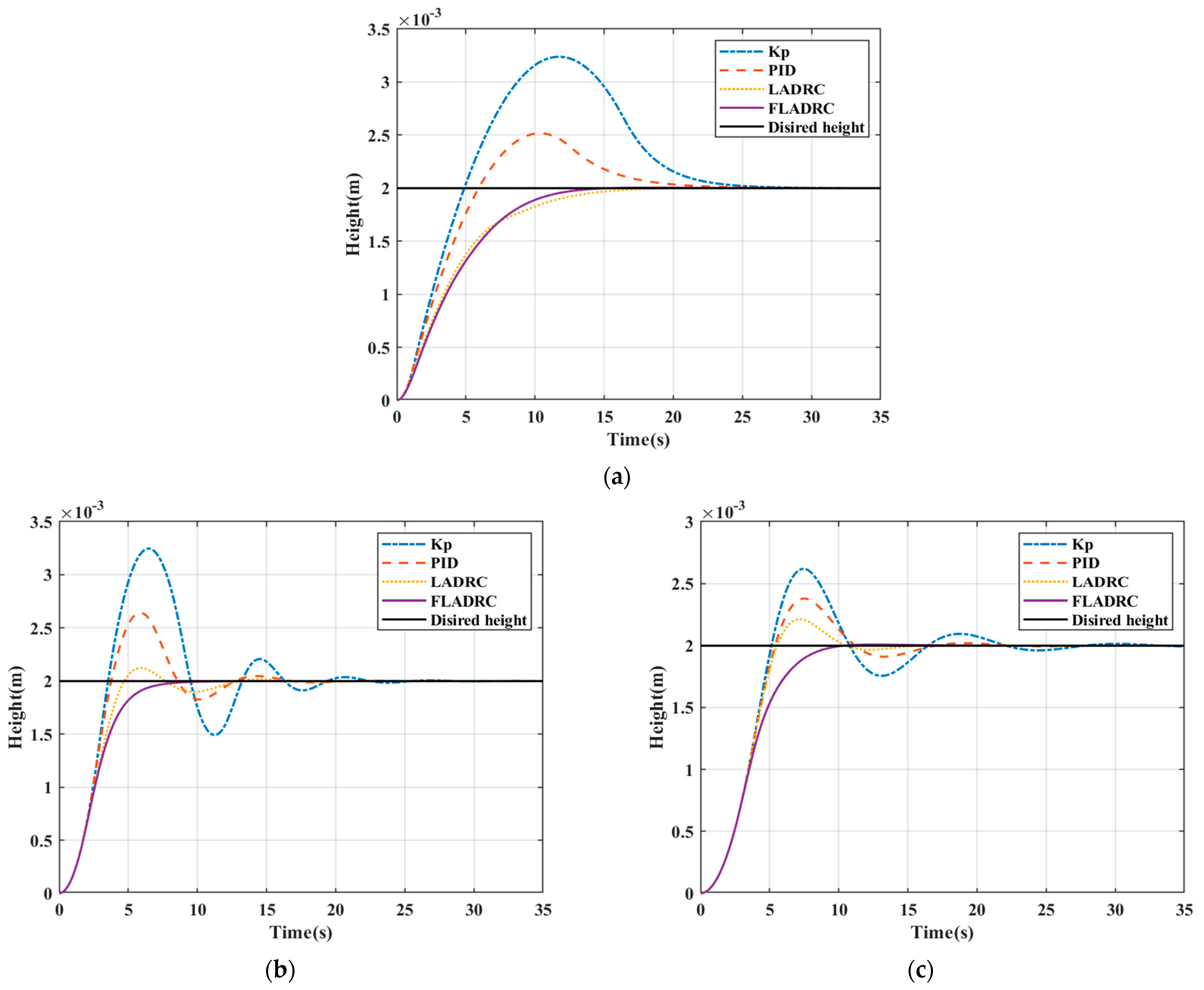
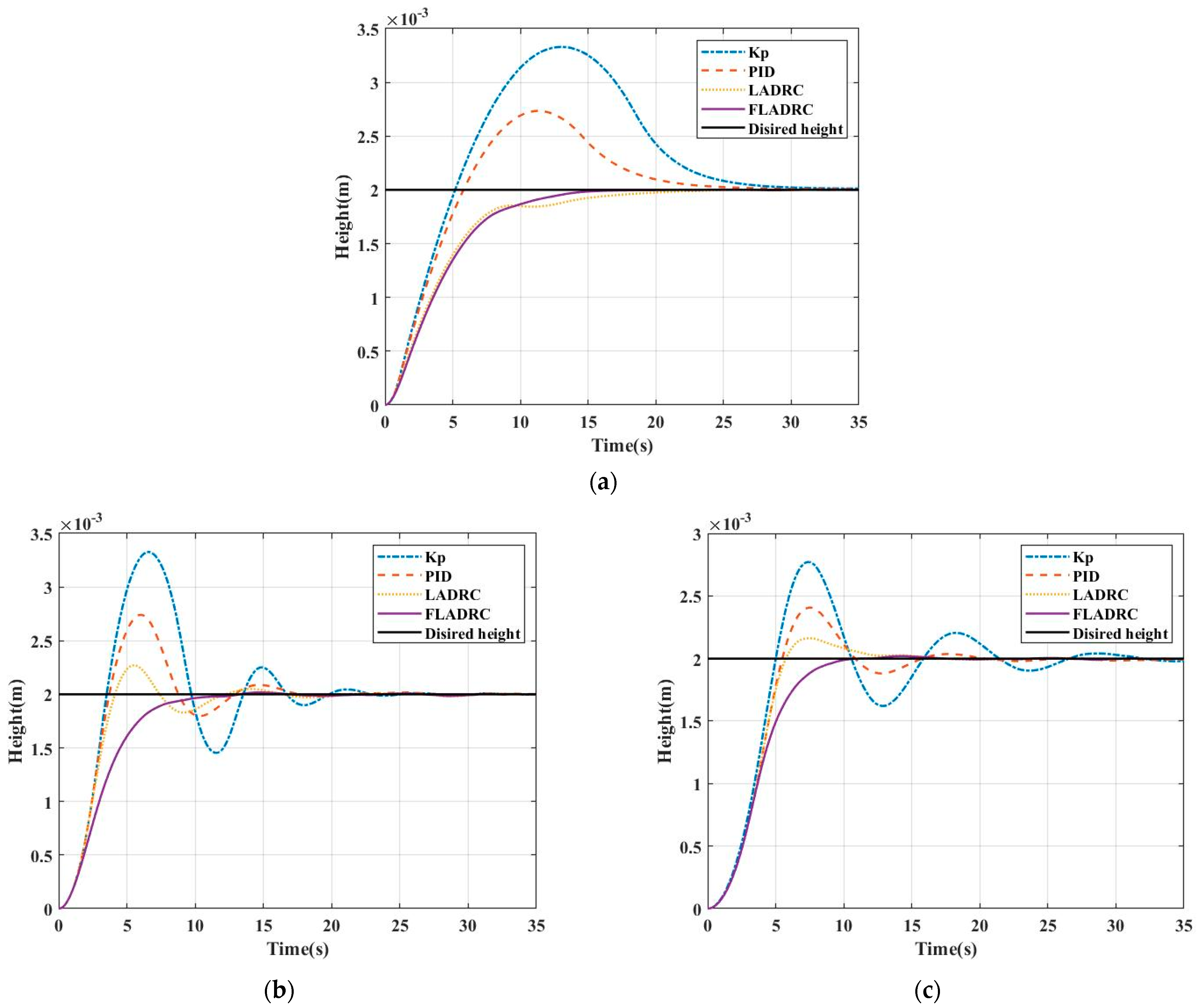
Considering that in the actual working process of an absolute pressure piston manometer, the piston has to rise as quickly as possible and be stabilized in the desired position, the desired value of the piston height of the system is taken as the input signal for the simulation, which is uniformly set to a 2 mm step signal, the output signal is the real-time piston height of the piston, the simulation time is set to 35 s, and the error band is taken to be $\pm 2\mathrm{\%}$ of the desired height. To facilitate visual analysis, the stable convergence time t_s, the integral IAE of the absolute value of the actual error, and the maximum overshoot rate 6% are chosen as performance indicators in this paper. The real-time height profile of the piston is shown in Figure 5, and the experimental results of the selected performance metrics are shown in Figure 6 and

Table 6. Stable convergence time t_s(s).

Conditions	Kp	PID	LADRC	FLADRC
0.1 MPa	23.36	19.58	14.87	12.37
3 MPa	18.72	14.76	11.84	8.54
6 MPa	20.98	15.79	12.04	8.67

.

As shown in Figure 5 the FLADRC-controlled pistons all rise at a rate less than Kp, PID, and LADRC, but it is clear from Table 6 that the FLADRC-controlled pistons have the shortest stabilization time, the LADRC has the second shortest stabilization time and the Kp and PID have a longer stabilization time. As can be seen from Figure 6a, the IAE of the FLADRC is not very different from the LADRC overall, with the smallest IAE for the FLADRC at the 0.1 MPa and 3 MPa operating points. At the 6 MPa pressure operating point, the IAE of FLADRC is slightly greater than that of LADRC, but in Figure 6b, it can be seen that FLADRC is the best at suppressing overshoot, with a maximum overshoot of zero at the 0.1 MPa operating point and far less at the 3 MPa and 6 MPa pressure operating points than the other three control strategies. It can be concluded that the FLADRC control strategy proposed in this paper has the best stability performance in the equilibrium control of absolute pressure piston manometers.

4.3. Experimental Analysis of Interference Immunity Performance

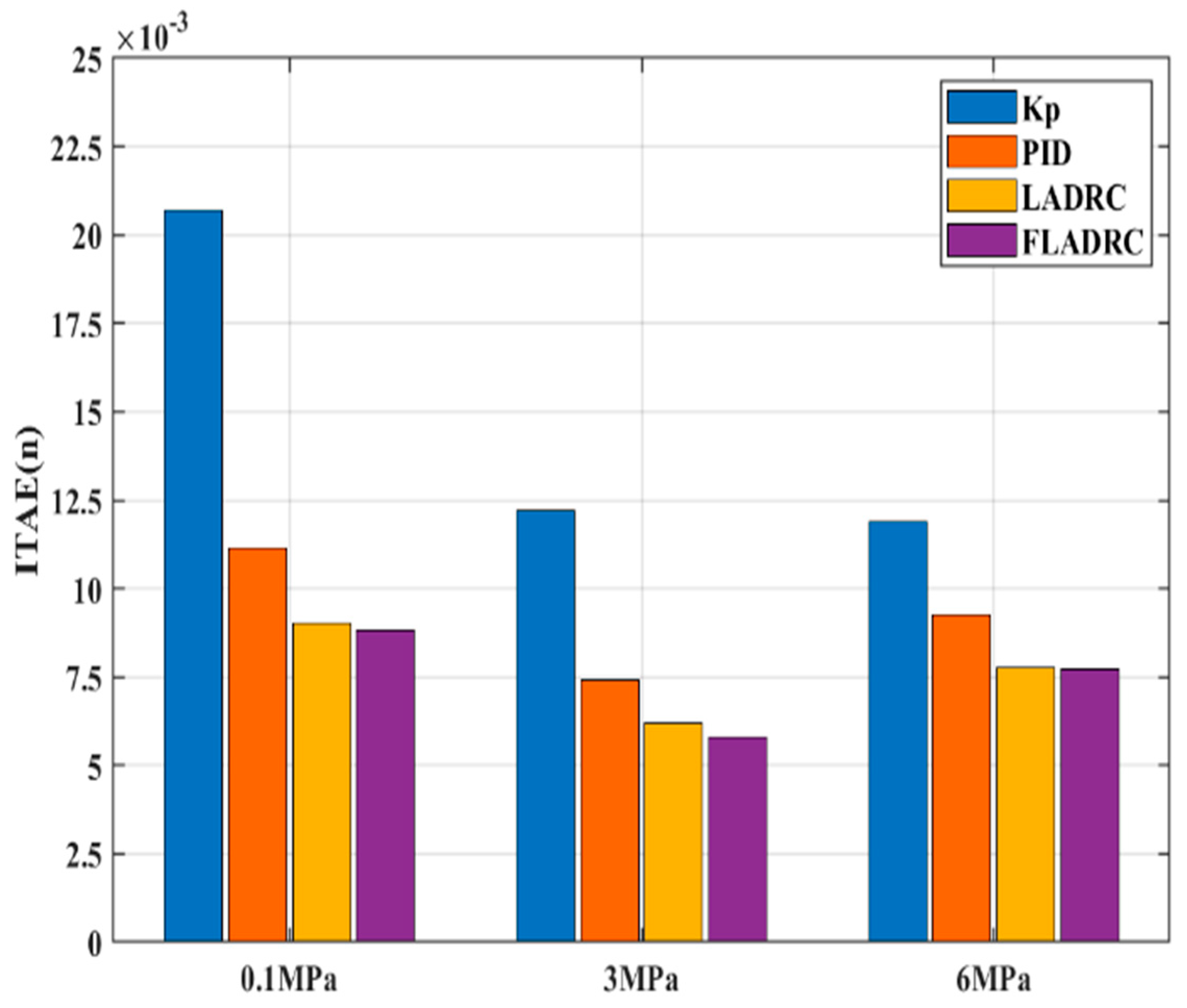
Absolute pressure piston manometers can be subject to many external disturbances during actual operation, such as temperature and humidity, atmospheric pressure, and electromagnetic fluctuations in the environment. Therefore, in the system interference immunity experiments, the system parameters, as well as the controller parameters, are kept constant, and the actual disturbance is assumed to be a time-varying white noise signal, which is added to the input flow of the system model, and its amplitude is set according to the gas incoming and outgoing flow limits at the specific pressure operating point. The corresponding simulation results are shown in Figure 7. The stability time t_s(n) and the integral IAE_(n) of the absolute value of the steady-state error are taken as the steady-state performance indicators so that they are compared with the experimental results in the previous section, and the corresponding rates of change ζ% and δ% of the two are derived, which are the system interference immunity performance indicators chosen in this paper. The specific results for t_s(n) and IAE_(n) are shown in

Table 7. Stable convergence time t_s(n) (s).

Conditions	Kp	PID	LADRC	FLADRC
0.1 MPa	27.62	22.48	17.09	13.26
3 MPa	21.67	16.28	14.85	9.87
6 MPa	25.33	22.03	13.07	10.41

and Figure 8, and the corresponding rates of change are calculated in

Table 8. Rate of change of t_s (ζ%).

Conditions	Kp	PID	LADRC	FLADRC
0.1 MPa	18.23%	18.95%	14.92%	7.19%
3 MPa	15.76%	12.06%	11.74%	10.77%
6 MPa	21.97%	13.29%	8.33%	6.22%

and

Table 9. The rate of change of IAE (δ%).

Conditions	Kp	PID	LADRC	FLADRC
0.1 MPa	19.21%	10.44%	3.35%	1.51%
3 MPa	15.34%	9.16%	7.63%	2.68%
6 MPa	16.47%	9.79%	4.44%	1.24%

.

It can be seen from Figure 7 that all control strategies stabilize within a certain time after the addition of time-varying disturbances. From Table 7 and Figure 8, it can be easily seen that the stabilization time and IAE(n) of all the control strategies increase to a greater or lesser extent due to the disturbance, but FLADRC still has the shortest stabilization time and the smallest IAE(n). This proves that the steady-state performance of FLADRC is still the best, even when disturbances are added.

The immunity performance index of each control strategy was obtained by calculation. As shown in Table 8, the rate of change of the steady-state time ζ is the smallest for FLADRC at all three different pressure operating points, followed by LADRC, while the steady-state times for PID and Kp are relatively more variable. As shown in Table 9, it is also evident that the FLADRC has the smallest rate of change of IAE, δ, followed by the LADRC, PID, and Kp, from largest to smallest. In summary, the steady-state performance of the FLADRC is least affected by time-varying disturbances, which means that the FLADRC has the relatively best interference immunity performance.

Remark 3. 

The immunity performance indicators ζ and δ are calculated as follows:

$$\left\{\begin{array}{l}\zeta =(t_{s(n)}-t_s)/t_s\\ \delta =(IA{E}_{(n)}-IAE)/IAE\end{array}\right.$$

(39)

4.4. Experimental Analysis of Engineering Energy Consumption

In the actual operation of the system, the inlet and outlet valves are the two actuators, respectively, and the corresponding instantaneous gas mass flow rate is the control quantity of the system. These two control quantities have been abstracted into a positive and negative input signal in Section 2 of the article, with a positive value representing the inlet valve working alone and vice versa for the outlet valve working alone. The control quantity input curves for the system in the steady-state performance experiments are shown in Figure 9.

As shown in Figure 9 at different pressure operating points, the FLADRC used in this paper has the smallest oscillation of the control quantity signal compared to the other three control strategies, which means that the switching frequency of the switching valve is lower. The number of switches between the two actuators, the inlet and outlet valves, is less. This reduces the energy consumption of the actuator operation, reduces the wear of the valve stems in the switching valves, increases the overall actuator life, and reduces the possibility of mechanical errors after long periods of system operation.

5. Conclusions

This paper takes into account the fact that absolute pressure piston manometers are subject to many internal uncertainties and non-linearities during actual operation and that the control performance of the system equilibrium needs to be improved urgently. Therefore, this paper proposes a FLADRC-based equilibrium control method for absolute pressure piston gauges. The control method combines the advantages of LADRC and fuzzy control to effectively estimate and compensate for real-time internal and external disturbances in the system and to achieve adaptive online adjustment of the control parameters. In the contemporary field of control, very little research has been carried out on the controlled systems mentioned in this paper, so a linearized theoretical model of the absolute pressure piston manometer was first developed. Furthermore, the FLADRC controller was designed according to the model, and the initialization parameters were determined by a search for merit. In addition, the stability of the control system was also analyzed. Finally, the simulation is verified in MATLAB’s Simulink environment, and its experimental results are compared and analyzed with Kp, PID, and LADRC. The results show that the FLADRC control strategy proposed in this paper has the advantages of short stability time, small overshoot, strong anti-interference capability, and low input energy consumption, verifying that it has important engineering application value for absolute pressure piston manometers.

In future work, it is intended to further commercialize the absolute pressure piston manometer by designing an automatic matching system for the pressure operating point and the corresponding control parameters. An attempt is also made to apply the FLADRC strategy to a piston manometer with a liquid as the working medium and to carry out the corresponding performance verification.

References

1. Yang, Y.; Driver, R.G.; Quintavalle, J.S.; Scherschligt, J.; Schlatter, K.; Ricker, J.E.; Strouse, G.F.; Olson, D.A.; Hendricks, J.H. An integrated and automated calibration system for pneumatic piston gauges. Measurement 2018, 134, 1–5. [Google Scholar] [CrossRef]
2. Schmidt, J.W.; A Tison, S.; Ehrlich, C.D. Model for drag forces in the crevice of piston gauges in the viscous-flow and molecular-flow regimes. Metrologia 1999, 36, 565–570. [Google Scholar] [CrossRef] [Green Version]
3. Welch, B.; Edsinger, R.; Bean, V.; Ehrlich, C. The reduction of uncertainties for absolute piston gauge pressure measurements in the atmospheric pressure range. J. Res. Natl. Inst. Stand. Technol. 1989, 94, 343–346. [Google Scholar] [CrossRef] [PubMed]
4. Li, C.; Jing, H.; Bao, J.; Sun, S.; Wang, R. Robust H fault tolerant control for quadrotor attitude regulation. Proc. Inst. Mech. Eng. Part I J. Syst. Control Eng. 2018, 232, 1302–1313. [Google Scholar] [CrossRef]
5. Romero, A.; Sun, S.; Foehn, P.; Scaramuzza, D. Model Predictive Contouring Control for Time-Optimal Quadrotor Flight. IEEE Trans. Robot. 2022, 38, 3340–3356. [Google Scholar] [CrossRef]
6. Wang, X.; Dong, H.; Sun, X.; Yao, X. PD control of inverted pendulum based on adaptive fuzzy compensation. J. Intell. Fuzzy Syst. 2016, 31, 3013–3019. [Google Scholar] [CrossRef]
7. Sharma, A.K.; Bhushan, B. Comparison of various fuzzy sliding mode based controller on single link inverted pendulum. J. Intell. Fuzzy Syst. 2022, 42, 679–688. [Google Scholar] [CrossRef]
8. Semenov, M.E.; Solovyov, A.M.; Popov, M.A.; Meleshenko, P.A. Coupled inverted pendulums: Stabilization problem. Arch. Appl. Mech. 2017, 88, 517–524. [Google Scholar] [CrossRef]
9. Liu, Y.; Huang, X.; Wang, T.; Zhang, Y.; Li, X. Nonlinear dynamics modeling and simulation of two-wheeled self-balancing vehicle. Int. J. Adv. Robot. Syst. 2016, 13, 156–171. [Google Scholar] [CrossRef] [Green Version]
10. Huang, C.-N. The Development of Self-Balancing Controller for One-Wheeled Vehicles. Engineering 2010, 2, 212–219. [Google Scholar] [CrossRef] [Green Version]
11. Qu, L.; Qiao, W.; Qu, L. Active-Disturbance-Rejection-Based Sliding-Mode Current Control for Permanent-Magnet Synchronous Motors. IEEE Trans. Power Electron. 2020, 36, 751–760. [Google Scholar] [CrossRef]
12. Tarczewski, T.; Grzesiak, L.M. Constrained State Feedback Speed Control of PMSM Based on Model Predictive Approach. IEEE Trans. Ind. Electron. 2015, 63, 3867–3875. [Google Scholar] [CrossRef]
13. Lee, D.; Cheon, Y.; Ryu, J.-H.; Lee, I.-B. An MCFC operation optimization strategy based on PID auto-tuning control. Int. J. Hydrogen Energy 2017, 42, 25518–25530. [Google Scholar] [CrossRef]
14. Rakhtala, S.; Roudbari, E.S. Fuzzy PID control of a stand-alone system based on PEM fuel cell. Int. J. Electr. Power Energy Syst. 2016, 78, 576–590. [Google Scholar] [CrossRef]
15. Gün, A. Attitude control of a quadrotor using PID controller based on differential evolution algorithm. Expert Syst. Appl. 2023, 229, 412–424. [Google Scholar] [CrossRef]
16. Nocoń, Ł.; Koruba, Z. Modified linear-quadratic regulator used for controlling anti-tank guided missile in vertical plane. J. Theor. Appl. Mech. 2020, 58, 723–732. [Google Scholar] [CrossRef]
17. Borrelli, F.; Keviczky, T. Distributed LQR Design for Identical Dynamically Decoupled Systems. IEEE Trans. Autom. Control 2008, 53, 1901–1912. [Google Scholar] [CrossRef]
18. Tingting, Y.; Aijun, L.; Taimoor, M.; Amin, R.U. High AOA short landing robust control for an aircraft. Aircr. Eng. Aerosp. Technol. 2018, 91, 38–49. [Google Scholar] [CrossRef]
19. Pan, S. Robust control of gyro stabilized platform driven by ultrasonic motor. Sens. Actuators A Phys. 2017, 261, 280–287. [Google Scholar] [CrossRef]
20. Abbasi, S.M.M.; Jalali, A. Fuzzy tracking control of fuzzy linear dynamical systems. ISA Trans. 2020, 97, 102–115. [Google Scholar] [CrossRef]
21. Yoon, J.H.; Bak, G.-M.; Bae, Y. Fuzzy Control for Chaotic Confliction Model. Int. J. Fuzzy Syst. 2020, 22, 1961–1971. [Google Scholar] [CrossRef]
22. Lu, Y. Adaptive-fuzzy control compensation design for direct adaptive fuzzy control. IEEE Trans. Fuzzy Syst. 2018, 26, 3222–3231. [Google Scholar] [CrossRef]
23. Canciello, G.; Cavallo, A.; Cucuzzella, M.; Ferrara, A. Fuzzy scheduling of robust controllers for islanded DC microgrids applications. Int. J. Dyn. Control. 2019, 7, 690–700. [Google Scholar] [CrossRef] [Green Version]
24. Zhao, Z.; Liu, Z.; He, W.; Hong, K.-S.; Li, H.-X. Boundary adaptive fault-tolerant control for a flexible Timoshenko arm with backlash-like hysteresis. Automatica 2021, 130, 109690. [Google Scholar] [CrossRef]
25. Sang, H.; Zhou, Y.; Sun, X.; Yang, S. Heading tracking control with an adaptive hybrid control for under actuated underwater glider. ISA Trans. 2018, 80, 554–563. [Google Scholar] [CrossRef] [PubMed]
26. Muñoz-Vázquez, A.J.; Fernández-Anaya, G.; Meléndez-Vázquez, F.; Torres, J.D.S. Generalised conformable sliding mode control. Math. Methods Appl. Sci. 2021, 45, 1687–1699. [Google Scholar] [CrossRef]
27. Ma, H.; Wu, J.; Xiong, Z. Discrete-time sliding-mode control with improved quasi-sliding-mode domain. IEEE Trans. Ind. Electron. 2016, 63, 6292–6304. [Google Scholar] [CrossRef]
28. Canciello, G.; Cavallo, A.; Schiavo, A.L.; Russo, A. Multi-objective adaptive sliding manifold control for More Electric Aircraft. ISA Trans. 2020, 107, 316–328. [Google Scholar] [CrossRef]
29. Nichols, G.P.; Fontenot, J.D.; Gibbons, J.P.; Sanders, M. Evaluation of volumetric modulated Arc therapy for postmastectomy treatment. Radiat. Oncol. 2014, 9, 66. [Google Scholar] [CrossRef] [Green Version]
30. Wang, F.; Chen, K.; Zhen, S.; Zheng, H.; Chen, X.; Chen, F. Optimal design of Udwadia–Kalaba theory-based adaptive robust control for permanent magnet linear synchronous motor. J. Vib. Control 2023, 10775463221149086. [Google Scholar] [CrossRef]
31. Nadda, S.; Swarup, A. On adaptive sliding mode control for improved quadrotor tracking. J. Vib. Control 2017, 24, 3219–3230. [Google Scholar] [CrossRef]
32. Jain, A.; Sharma, A.; Jately, V.; Azzopardi, B.; Choudhury, S. Real-Time Swing-Up Control of Non-Linear Inverted Pendulum Using Lyapunov Based Optimized Fuzzy Logic Control. IEEE Access 2021, 9, 50715–50726. [Google Scholar] [CrossRef]
33. Luo, Z.; Xu, L. Research on LQR controller of control torque gyro self-balancing vehicle based on QPSO optimization. J. Phys. Conf. Ser. 2022, 2258, 012071. [Google Scholar] [CrossRef]
34. Han, J. From PID to Active Disturbance Rejection Control. IEEE Trans. Ind. Electron. 2009, 56, 900–906. [Google Scholar] [CrossRef]
35. Gao, Z. Scaling and bandwidth-parameterization based controller tuning. In Proceedings of the 2003 American Control Conference, Denver, CO, USA, 4–6 June 2003; pp. 4989–4996. [Google Scholar] [CrossRef]
36. Yuan, C.; Zhou, X.; Ma, Y.; Gao, Z.; Zhou, Y.; Wang, C. Improved Application of Third-Order LADRC in Wind Power Inverter. Energies 2020, 13, 4412. [Google Scholar] [CrossRef]
37. Wang, Z.; Zhao, T. Based on robust sliding mode and linear active disturbance rejection control for attitude of quadrotor load UAV. Nonlinear Dyn. 2022, 108, 3485–3503. [Google Scholar] [CrossRef]
38. Zeng, J.; Huang, Z.; Huang, Y.; Qiu, G.; Li, Z.; Yang, L.; Yu, T.; Yang, B. Modified linear active disturbance rejection control for microgrid inverters: Design, analysis, and hardware implementation. Int. Trans. Electr. Energy Syst. 2019, 29, e12060. [Google Scholar] [CrossRef]
39. Ramasamy, K.; Rathinasamy, S.; Kwon, O.M.; Palanisamy, S. Robust tracking control design for fractional-order interval type-2 fuzzy systems. Nonlinear Dyn. 2021, 107, 3611–3628. [Google Scholar] [CrossRef]
40. Qiu, T.; Dai, H.; Lei, Y.; Liu, Y. Effects of valve needle speed on flow characteristics in control valve for unit pump fuel system. Adv. Mech. Eng. 2018, 10, 378–389. [Google Scholar] [CrossRef] [Green Version]
41. Kavikumar, R.; Kwon, O.-M.; Kaviarasan, B.; Sakthivel, R. Antidisturbance Control Design for Interval Type-2 Fuzzy Stochastic Systems with Input Quantization. IEEE Trans. Fuzzy Syst. 2022, 31, 1806–1818. [Google Scholar] [CrossRef]
42. Bobovnik, G.; Kutin, J. Correlation of the leakage flow rate with pressure changes in a clearance-sealed piston prover. Flow Meas. Instrum. 2020, 74, 101785. [Google Scholar] [CrossRef]
43. Yu, B.; Shen, A.; Chen, B.; Luo, X.; Tang, Q.; Xu, J.; Zhu, M. A Compensation Strategy of Flux Linkage Observer in SPMSM Sensorless Drives Based on Linear Extended State Observer. IEEE Trans. Energy Convers. 2021, 37, 824–831. [Google Scholar] [CrossRef]
44. Liang, Q.; Wang, C.; Pan, J.; Wei, Y.; Wang, Y. Identification of linear self-adjoint control parameters b0 and parameter tuning laws. Control Decis. Mak. 2015, 30, 1691–1695. [Google Scholar]
45. Ren, Q.; Bigras, P. A Highly Accurate Model-Free Motion Control System with a Mamdani Fuzzy Feedback Controller combined with a TSK Fuzzy Feed-forward Controller. J. Intell. Robot. Syst. 2017, 86, 367–379. [Google Scholar] [CrossRef]
Figure 1. Schematic diagram of the structure of an absolute pressure piston manometer.
Actuators 12 00275 g001
Figure 2. Analysis of the forces on the combined weight section under different working conditions. (a) Piston rise; (b) Piston drop.
Actuators 12 00275 g002
Figure 3. Schematic diagram of the second-order LADRC structure.
Actuators 12 00275 g003
Figure 4. Schematic diagram of the FLADRC structure.
Actuators 12 00275 g004
Figure 5. Real-time piston height curves at three different pressure operating points. (a) 0.1 MPa; (b) 3 MPa; (c) 6 MPa.
Actuators 12 00275 g005
Figure 6. Comparison of the two performance indicators. (a) IAE; (b) σ%.
Actuators 12 00275 g006
Figure 7. Real-time piston height curves after disturbance at three different pressure operating points. (a) 0.1 MPa; (b) 3 MPa; (c) 6 MPa.
Actuators 12 00275 g007
Figure 8. Comparison chart for performance indicator IAE(n).
Actuators 12 00275 g008
Figure 9. Control volume input curves at three different pressure operating points. (a) 0.1 MPa; (b) 3 MPa; (c) 6 MPa.
Actuators 12 00275 g009