


LSTM-CNN Network-Based State-Dependent ARX Modeling and Predictive Control with Application to Water Tank System

Abstract
1. Introduction
- (1)
- The LSTM-ARX and LSTM-CNN-ARX models are proposed to describe the system’s nonlinear features.
- (2)
- The predictive controller was developed using the model’s pseudo-linear structure features.
- (3)
- Control comparison experiments were conducted on the water tank system, which is a commonly used industrial process control device, to validate the efficiency of the developed models and control algorithms. To our knowledge, there are currently no reports on using deep learning algorithms for nonlinear system modeling and the real-time control of actual industrial equipment. This study demonstrates how to establish deep learning-related models for nonlinear systems, design the MPC algorithms, and achieve real-time control rather than only doing a numerical simulation as in the relevant literature.
2. Related Work
2.1. SD-ARX Model
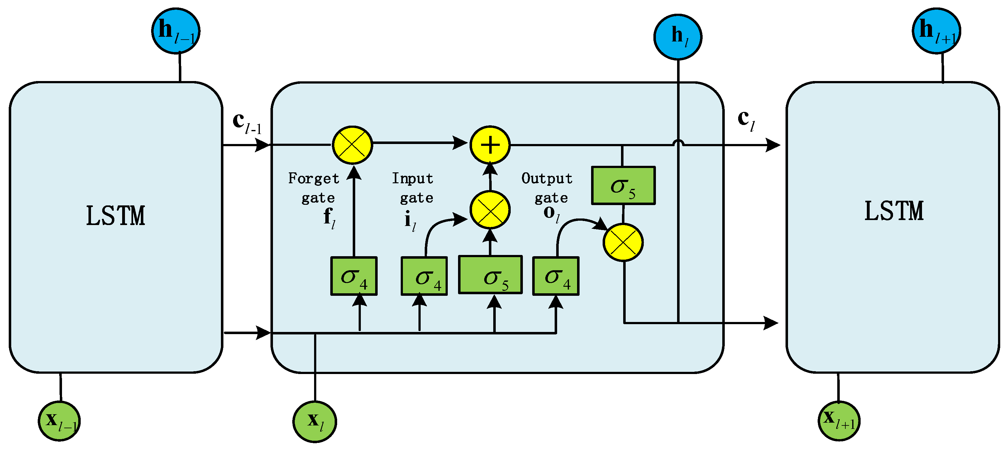
2.2. LSTM
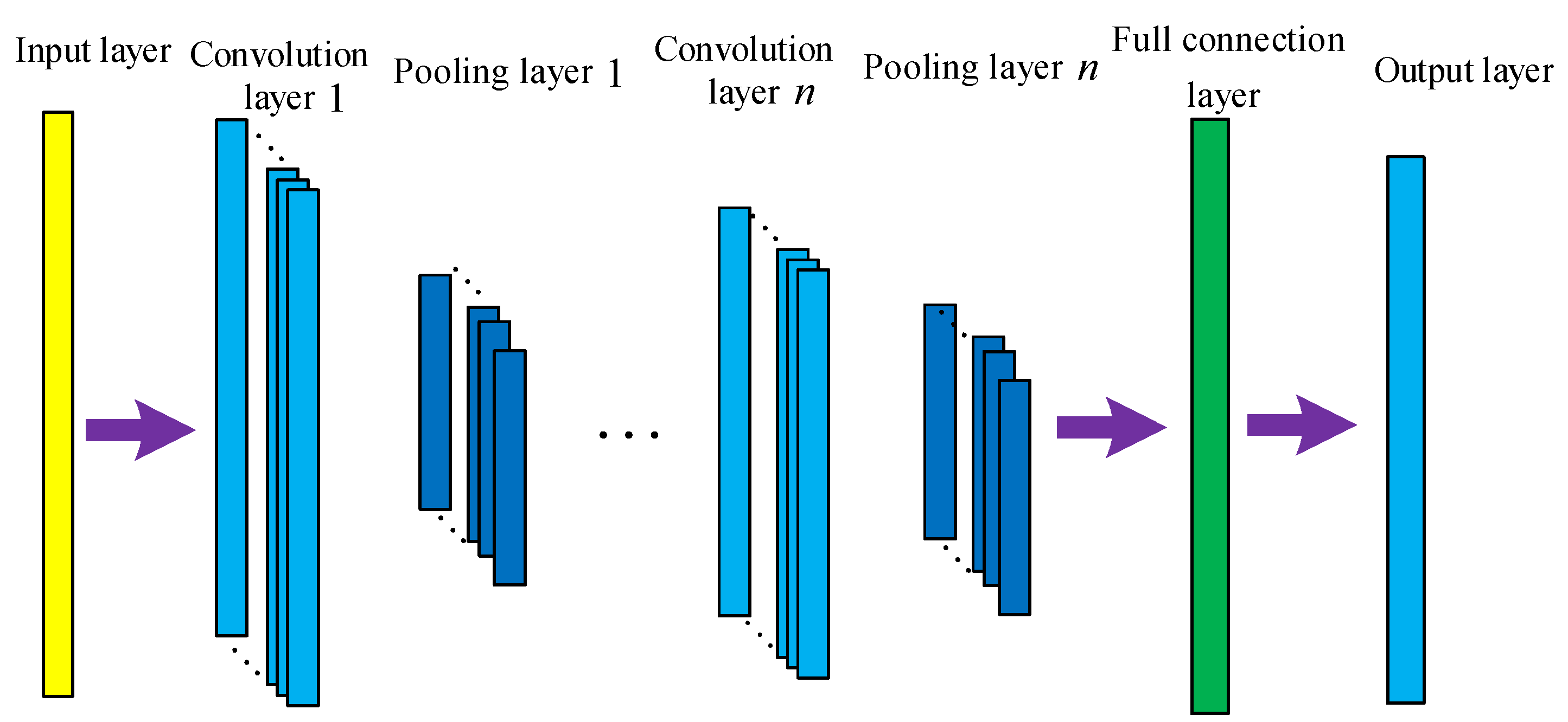
2.3. CNN
3. Hybrid Models
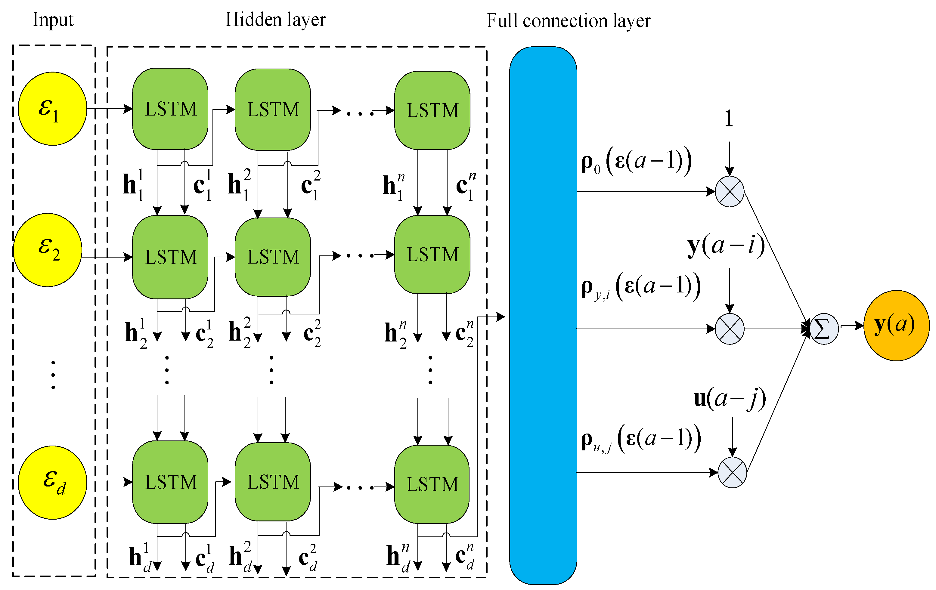
3.1. LSTM-ARX Model
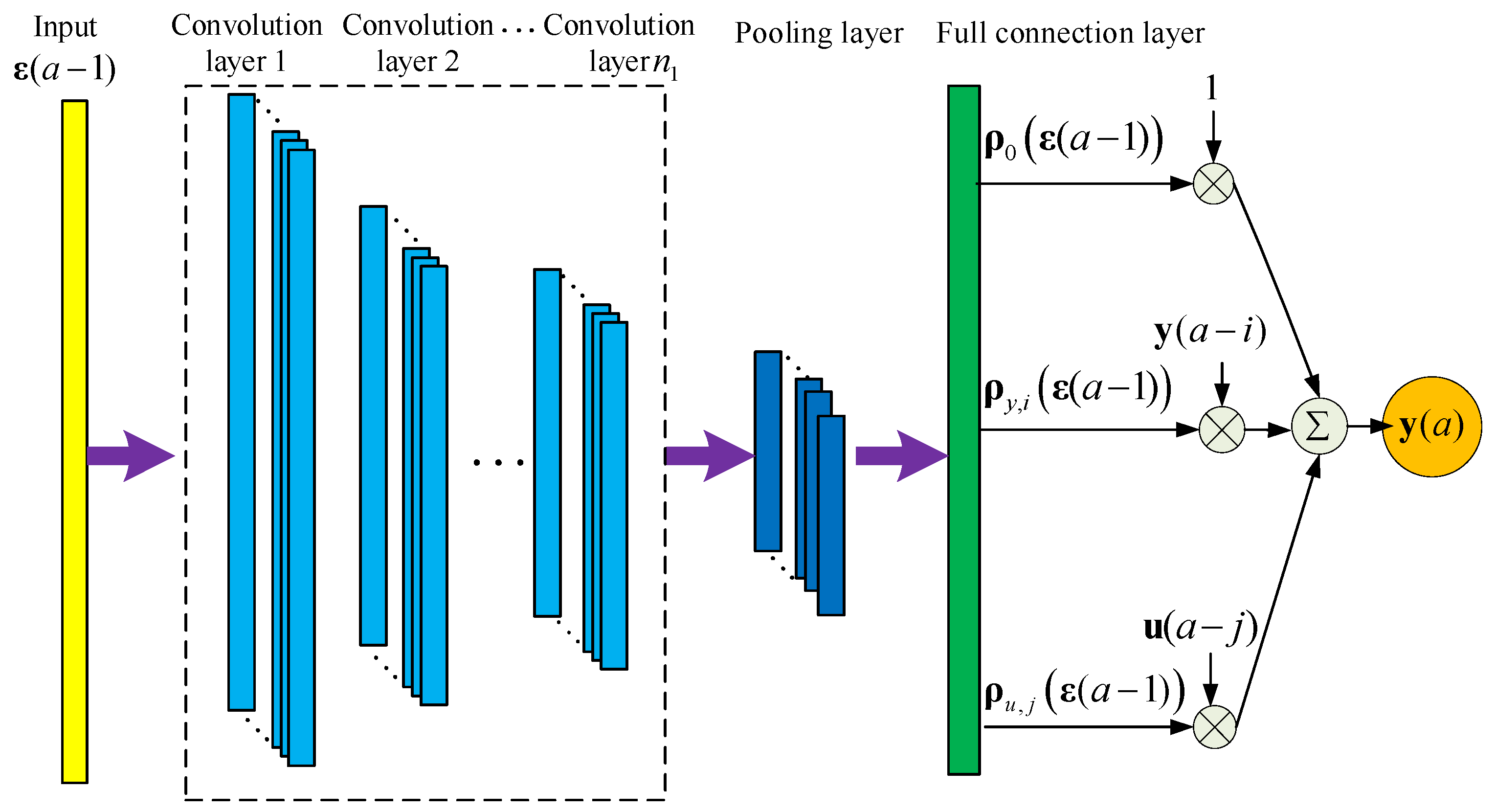
3.2. CNN-ARX Model
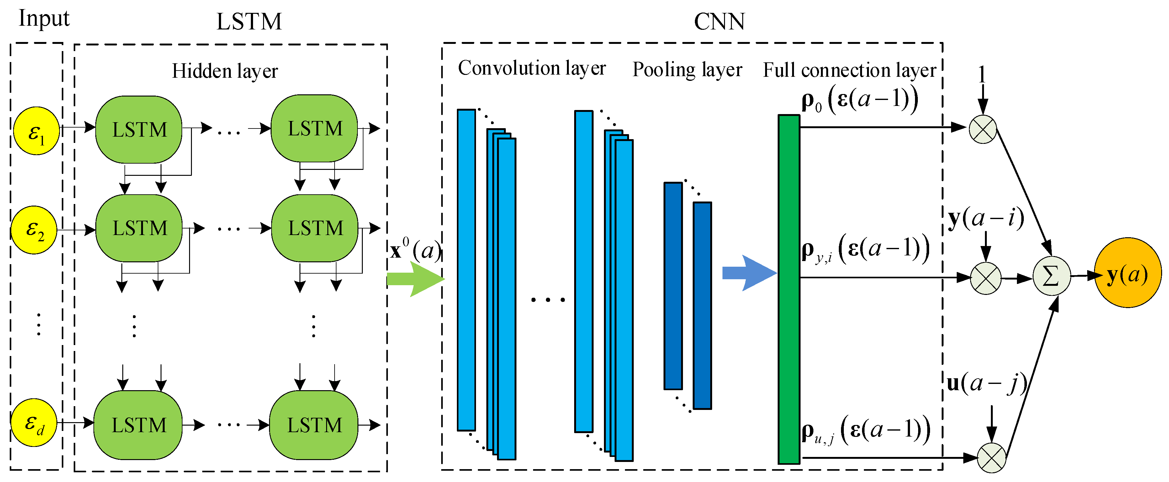
3.3. LSTM-CNN-ARX Model
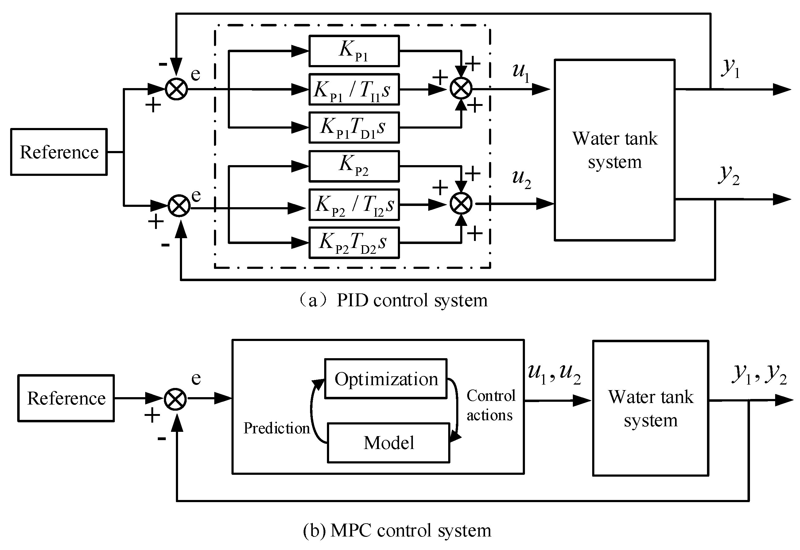
4. MPC Algorithm Design
5. Control Experiments
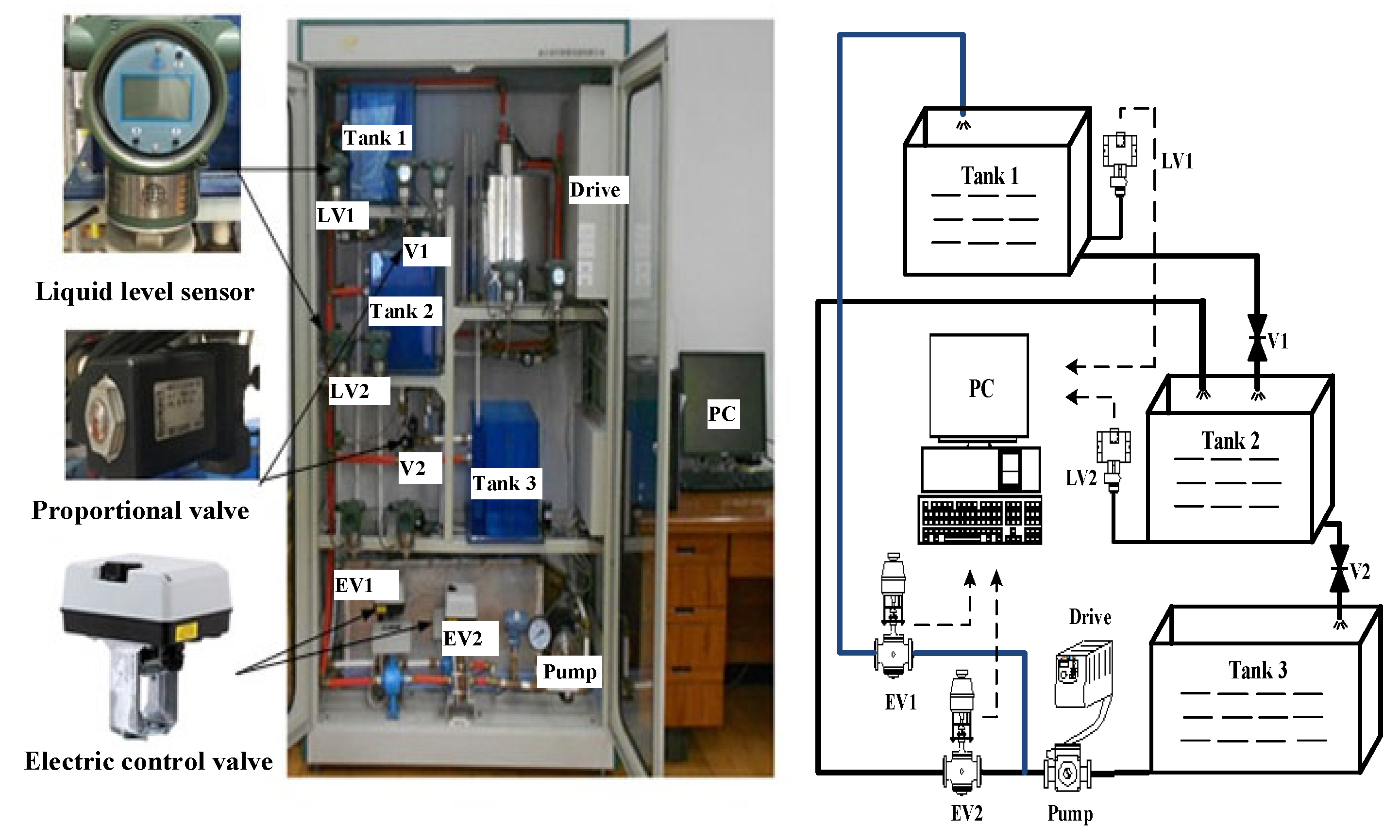
5.1. Water Tank System
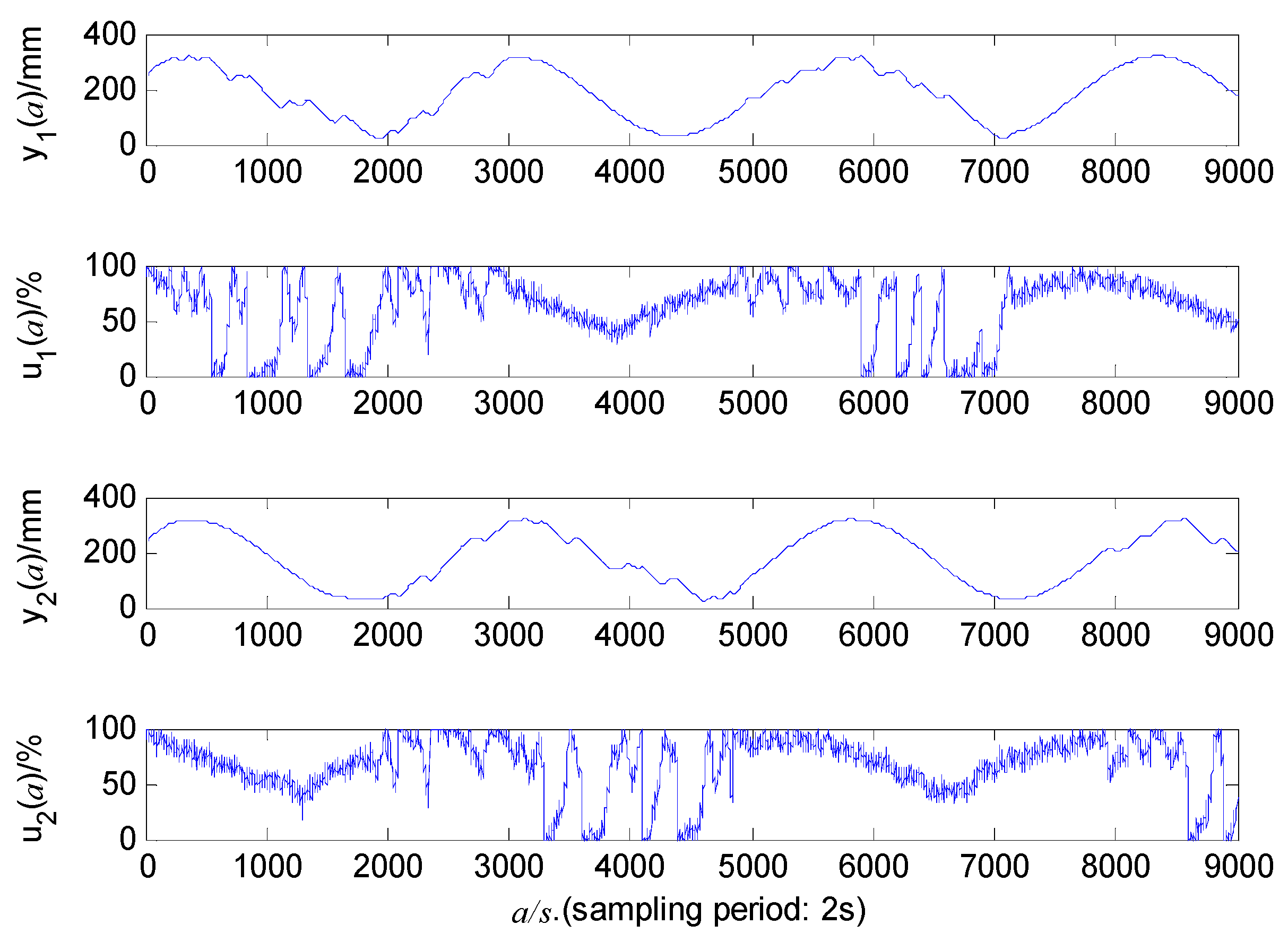
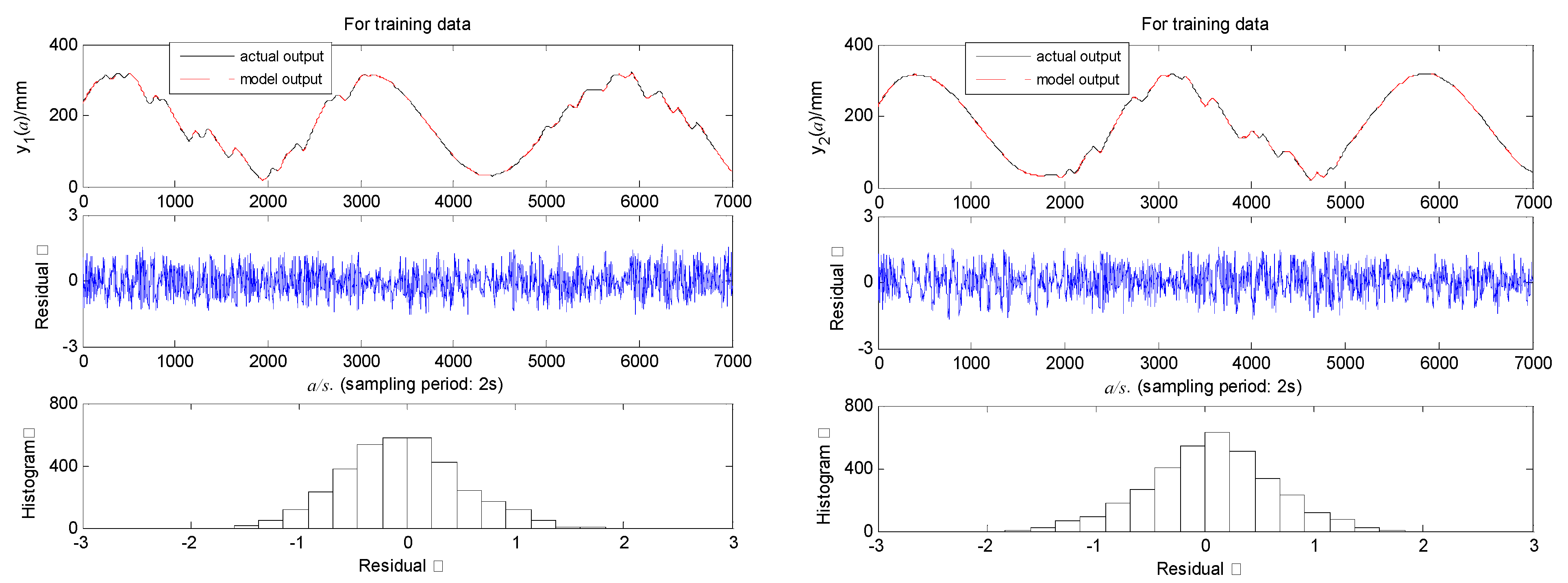
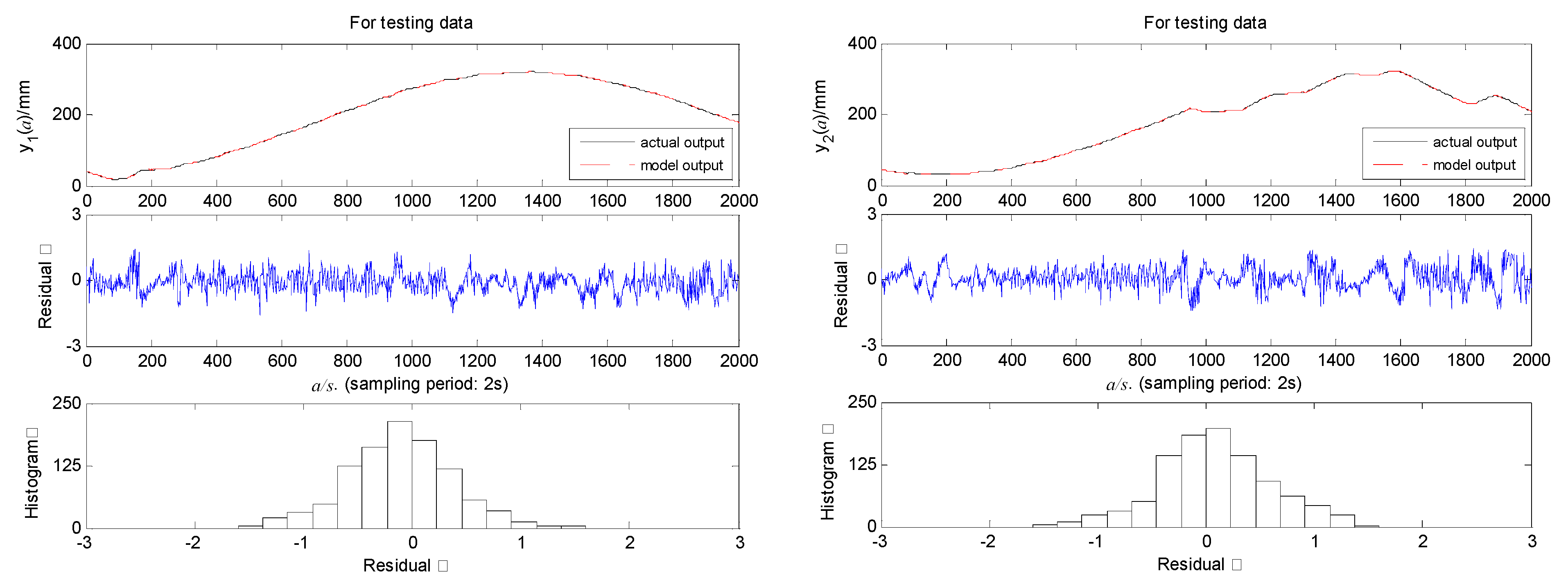
5.2. Estimation of Model
5.3. Real-Time Control Experiments
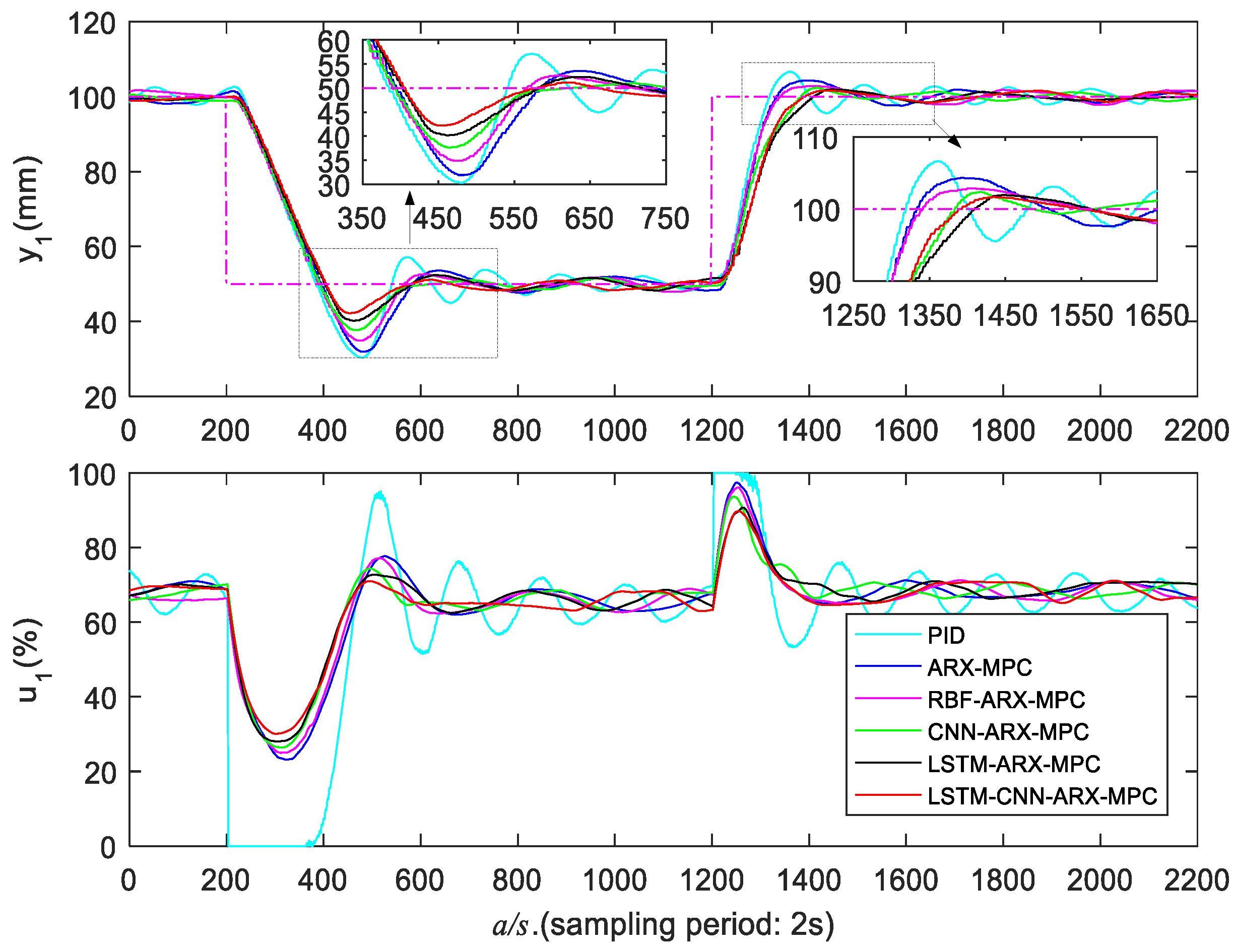
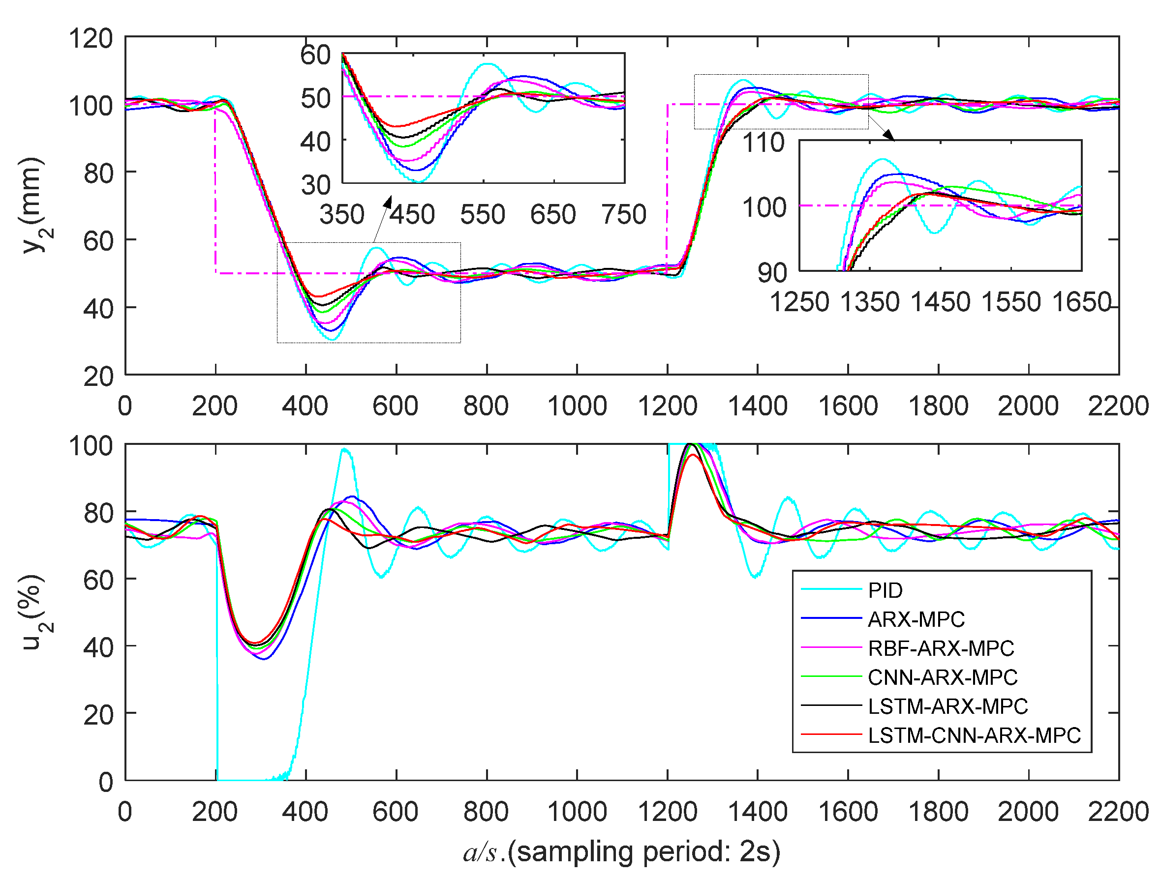
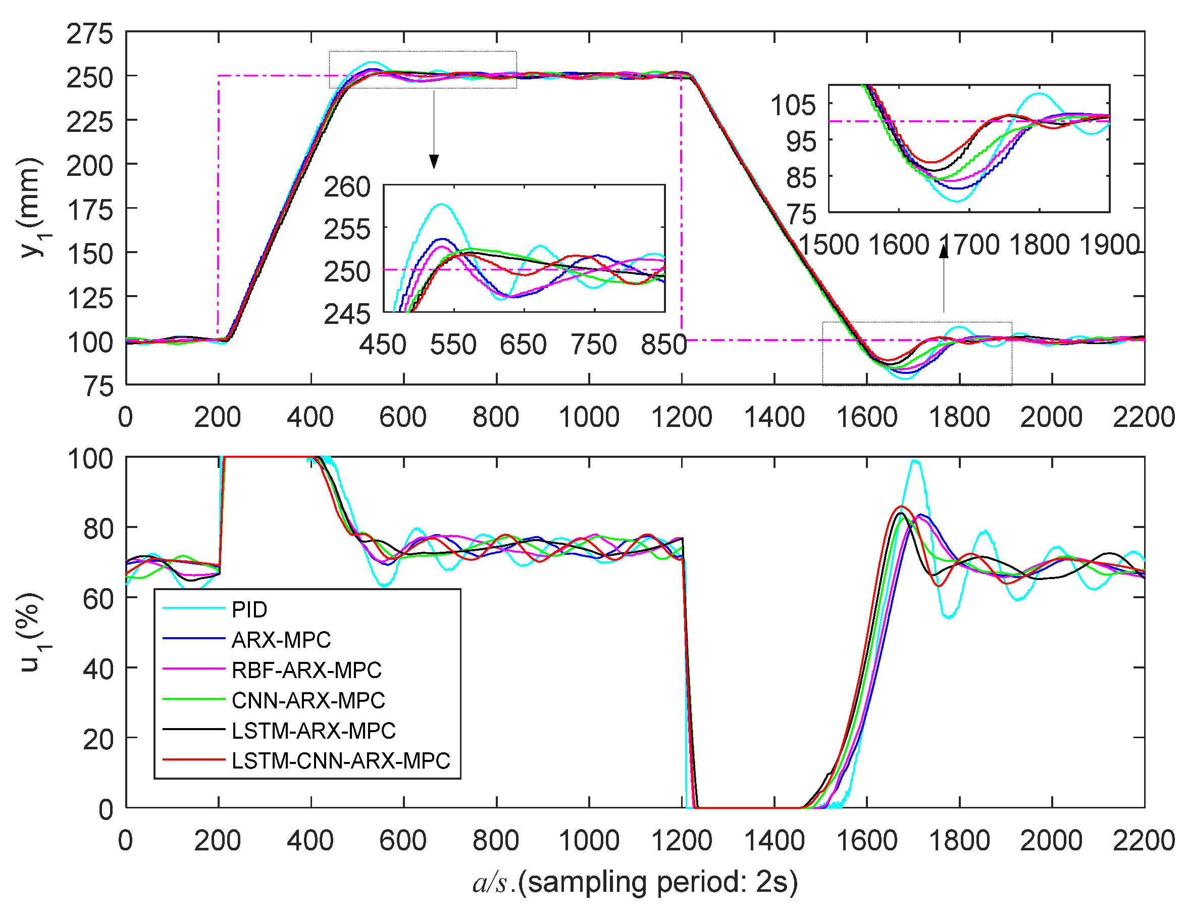
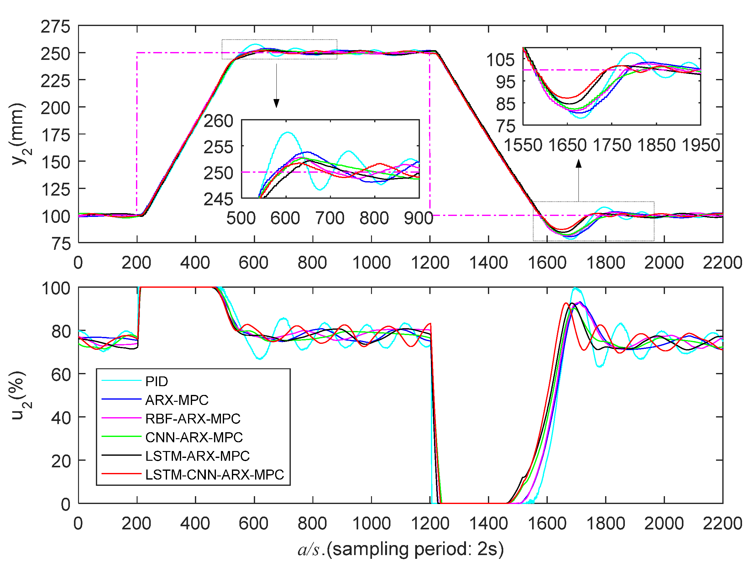
5.3.1. Low Liquid Level Zone Control Experiments
5.3.2. Medium Liquid Level Zone Control Experiments
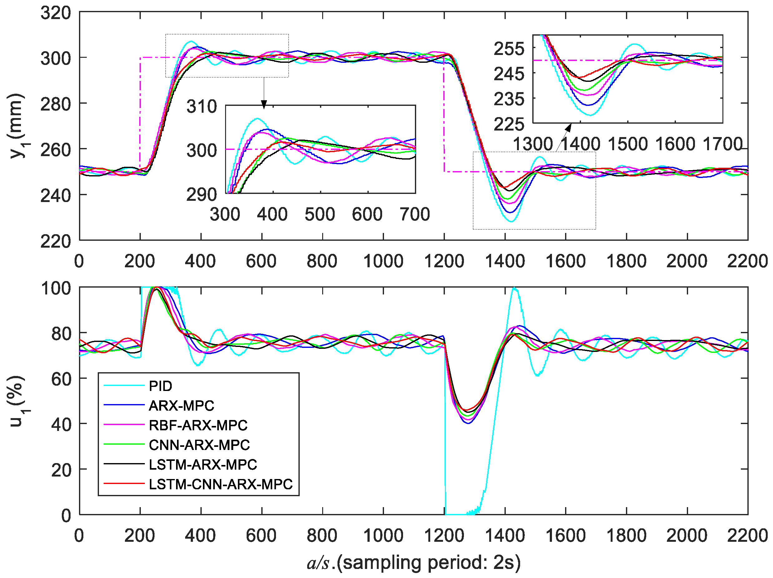
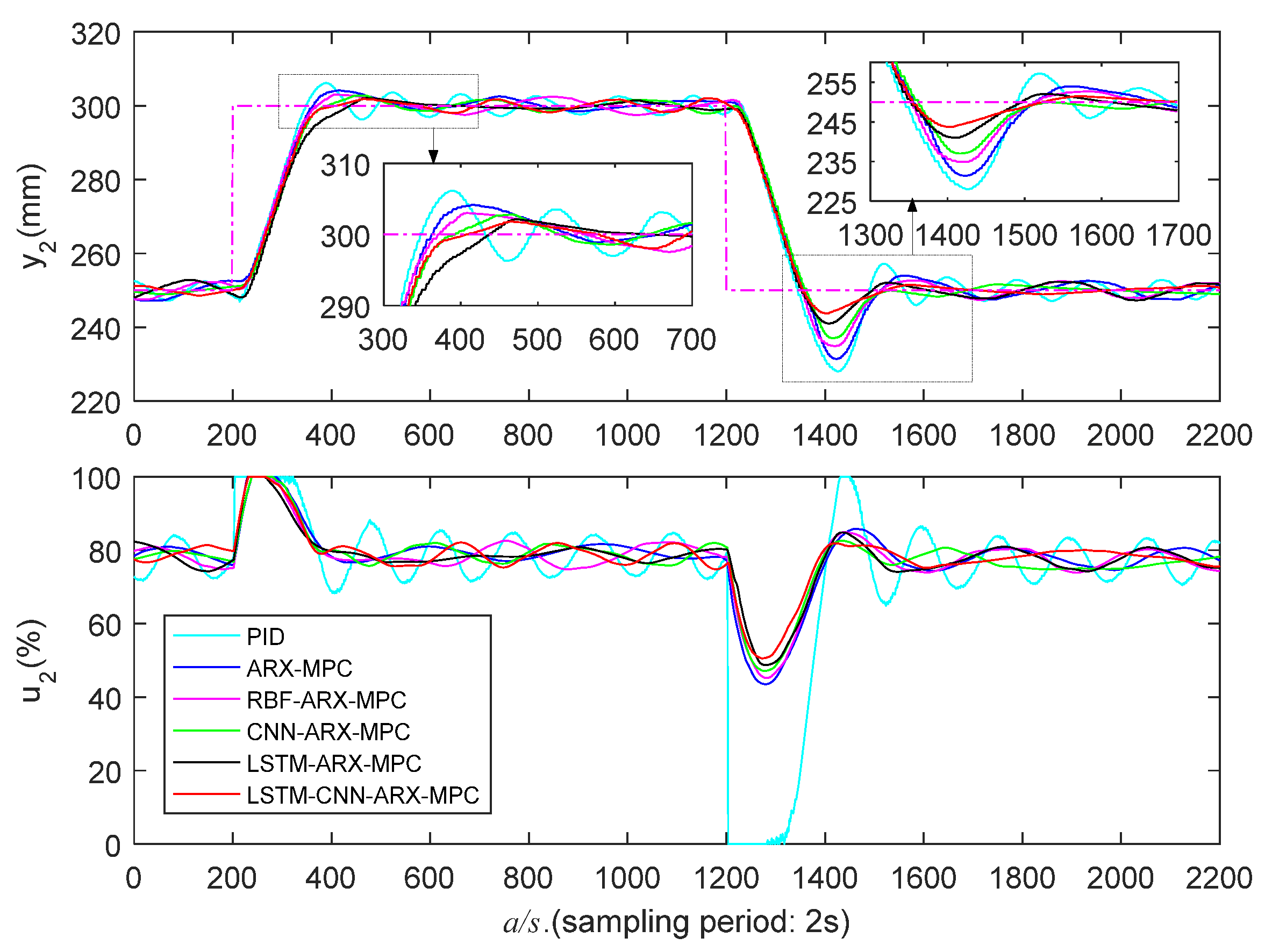
5.3.3. High Liquid Level Zone Control Experiments
6. Conclusions
Author Contributions
Funding
Institutional Review Board Statement
Informed Consent Statement
Data Availability Statement
Conflicts of Interest
References
- Mayne, D.Q. Model predictive control: Recent developments and future promise. Automatica 2014, 50, 2967–2986. [Google Scholar] [CrossRef]
- Elnawawi, S.; Siang, L.C.; O’Connor, D.L.; Gopaluni, R.B. Interactive visualization for diagnosis of industrial Model Predictive Controllers with steady-state optimizers. Control Eng. Pract. 2022, 121, 105056. [Google Scholar] [CrossRef]
- Kwapień, J.; Drożdż, S. Physical approach to complex systems. Phys. Rep. 2012, 515, 115–226. [Google Scholar] [CrossRef]
- Chen, H.; Jiang, B.; Ding, S.X.; Huang, B. Data-driven fault diagnosis for traction systems in high-speed trains: A survey, challenges, and perspectives. IEEE Trans. Intell. Transp. Syst. 2022, 23, 1700–1716. [Google Scholar] [CrossRef]
- Yu, W.; Wu, M.; Huang, B.; Lu, C. A generalized probabilistic monitoring model with both random and sequential data. Automatica 2022, 144, 110468. [Google Scholar] [CrossRef]
- Pareek, P.; Verma, A. Piecewise Linearization of Quadratic Branch Flow Limits by Irregular Polygon. IEEE Trans. Power Syst. 2018, 33, 7301–7304. [Google Scholar] [CrossRef]
- Ławryńczuk, M. Nonlinear predictive control of a boiler-turbine unit: A state-space approach with successive on-line model linearisation and quadratic optimisation. ISA Trans. 2017, 67, 476–495. [Google Scholar] [CrossRef] [PubMed]
- Qian, K.; Zhang, Y. Bilinear model predictive control of plasma keyhole pipe welding process. J. Manuf. Sci. Eng. 2014, 136, 31002. [Google Scholar] [CrossRef]
- Nie, Z.; Gao, F.; Yan, C.B. A multi-timescale bilinear model for optimization and control of HVAC systems with consistency. Energies 2021, 14, 400. [Google Scholar] [CrossRef]
- Shi, Y.; Yu, D.L.; Tian, Y.; Shi, Y. Air-fuel ratio prediction and NMPC for SI engines with modified Volterra model and RBF network. Eng. Appl. Artif. Intell. 2015, 45, 313–324. [Google Scholar] [CrossRef]
- Gruber, J.K.; Ramirez, D.R.; Limon, D.; Alamo, T. A convex approach for NMPC based on second order Volterra series models. Int. J. Robust Nonlinear Control 2015, 25, 3546–3571. [Google Scholar] [CrossRef]
- Chen, H.; Chen, Z.; Chai, Z.; Jiang, B.; Huang, B. A single-side neural network-aided canonical correlation analysis with applications to fault diagnosis. IEEE Trans. Cybern. 2021, 52, 9454–9466. [Google Scholar] [CrossRef]
- Chen, H.; Liu, Z.; Alippi, C.; Huang, B.; Liu, D. Explainable intelligent fault diagnosis for nonlinear dynamic systems: From unsupervised to supervised learning. IEEE Trans. Neural Netw. Learn. Syst. 2022. [Google Scholar] [CrossRef]
- Ding, B.; Wang, J.; Su, B. Output feedback model predictive control for Hammerstein model with bounded disturbance. IET Control. Theory Appl. 2022, 16, 1032–1041. [Google Scholar] [CrossRef]
- Raninga, D.; TK, R.; Velswamy, K. Explicit nonlinear predictive control algorithms for Laguerre filter and sparse least square support vector machine-based Wiener model. Trans. Inst. Meas. Control 2021, 43, 812–831. [Google Scholar] [CrossRef]
- Wang, Z.; Georgakis, C. Identification of Hammerstein-Weiner models for nonlinear MPC from infrequent measurements in batch processes. J. Process Control 2019, 82, 58–69. [Google Scholar] [CrossRef]
- Du, J.; Zhang, L.; Chen, J.; Li, J.; Zhu, C. Multi-model predictive control of Hammerstein-Wiener systems based on balanced multi-model partition. Math. Comput. Model. Dyn. Syst. 2019, 25, 333–353. [Google Scholar] [CrossRef]
- Peng, H.; Ozaki, T.; Haggan-Ozaki, V.; Toyoda, Y. A parameter optimization method for radial basis function type models. IEEE Trans. Neural Netw. 2003, 14, 432–438. [Google Scholar] [CrossRef]
- Zhou, F.; Peng, H.; Qin, Y.; Zeng, X.; Xie, W.; Wu, J. RBF-ARX model-based MPC strategies with application to a water tank system. J. Process Contr. 2015, 34, 97–116. [Google Scholar] [CrossRef]
- Peng, H.; Nakano, K.; Shioya, H. Nonlinear predictive control using neural nets-based local linearization ARX model—Stability and industrial application. IEEE Trans. Control Syst. Technol. 2006, 15, 130–143. [Google Scholar] [CrossRef]
- Kang, T.; Peng, H.; Zhou, F.; Tian, X.; Peng, X. Robust predictive control of coupled water tank plant. Appl. Intell. 2021, 51, 5726–5744. [Google Scholar] [CrossRef]
- Peng, H.; Ozaki, T.; Toyoda, Y.; Shioya, H.; Nakano, K.; Haggan-Ozaki, V.; Mori, M. RBF-ARX model-based nonlinear system modeling and predictive control with application to a NOx decomposition process. Control Eng. Pract. 2004, 12, 191–203. [Google Scholar] [CrossRef]
- Peng, H.; Wu, J.; Inoussa, G.; Deng, Q.; Nakano, K. Nonlinear system modeling and predictive control using the RBF nets-based quasi-linear ARX model. Control Eng. Pract. 2009, 17, 59–66. [Google Scholar] [CrossRef]
- Xu, W.; Peng, H.; Tian, X.; Peng, X. DBN based SD-ARX model for nonlinear time series prediction and analysis. Appl. Intell. 2020, 50, 4586–4601. [Google Scholar] [CrossRef]
- Inoussa, G.; Peng, H.; Wu, J. Nonlinear time series modeling and prediction using functional weights wavelet neural network-based state-dependent AR model. Neurocomputing 2012, 86, 59–74. [Google Scholar] [CrossRef]
- Mu, R.; Zeng, X. A review of deep learning research. KSII Trans. Internet Inf. Syst. 2019, 13, 1738–1764. [Google Scholar] [CrossRef]
- Lippi, M.; Montemurro, M.A.; Degli Esposti, M.; Cristadoro, G. Natural language statistical features of LSTM-generated texts. IEEE Trans. Neural Netw. Learn. Syst. 2019, 30, 3326–3337. [Google Scholar] [CrossRef]
- Shuang, K.; Tan, Y.; Cai, Z.; Sun, Y. Natural language modeling with syntactic structure dependency. Inf. Sci. 2020, 523, 220–233. [Google Scholar] [CrossRef]
- Shuang, K.; Li, R.; Gu, M.; Loo, J.; Su, S. Major-minor long short-term memory for word-level language model. IEEE Trans. Neural Netw. Learn. Syst. 2019, 31, 3932–3946. [Google Scholar] [CrossRef]
- Ying, W.; Zhang, L.; Deng, H. Sichuan dialect speech recognition with deep LSTM network. Front. Comput. Sci. 2020, 14, 378–387. [Google Scholar] [CrossRef]
- Jo, J.; Kung, J.; Lee, Y. Approximate LSTM computing for energy-efficient speech recognition. Electronics 2020, 9, 2004. [Google Scholar] [CrossRef]
- Oruh, J.; Viriri, S.; Adegun, A. Long short-term Memory Recurrent neural network for Automatic speech recognition. IEEE Access 2022, 10, 30069–30079. [Google Scholar] [CrossRef]
- Yang, B.; Yin, K.; Lacasse, S.; Liu, Z. Time series analysis and long short-term memory neural network to predict landslide displacement. Landslides 2019, 16, 677–694. [Google Scholar] [CrossRef]
- Hu, J.; Wang, X.; Zhang, Y.; Zhang, D.; Zhang, M.; Xue, J. Time series prediction method based on variant LSTM recurrent neural network. Neural Process. Lett. 2020, 52, 1485–1500. [Google Scholar] [CrossRef]
- Peng, L.; Zhu, Q.; Lv, S.X.; Wang, L. Effective long short-term memory with fruit fly optimization algorithm for time series forecasting. Soft Comput. 2020, 24, 15059–15079. [Google Scholar] [CrossRef]
- Langeroudi, M.K.; Yamaghani, M.R.; Khodaparast, S. FD-LSTM: A Fuzzy LSTM Model for Chaotic Time-Series Prediction. IEEE Intell. Syst. 2022, 37, 70–78. [Google Scholar] [CrossRef]
- Wu, Z.; Rincon, D.; Luo, J.; Christofides, P.D. Machine learning modeling and predictive control of nonlinear processes using noisy data. AICHE J. 2021, 67, e17164. [Google Scholar] [CrossRef]
- Terzi, E.; Bonassi, F.; Farina, M.; Scattolini, R. Learning model predictive control with long short-term memory networks. Int. J. Robust Nonlinear Control 2021, 31, 8877–8896. [Google Scholar] [CrossRef]
- Zarzycki, K.; Ławryńczuk, M. Advanced predictive control for GRU and LSTM networks. Inf. Sci. 2022, 616, 229–254. [Google Scholar] [CrossRef]
- Yu, W.; Zhao, C.; Huang, B. MoniNet with concurrent analytics of temporal and spatial information for fault detection in industrial processes. IEEE Trans. Cybern. 2021, 52, 8340–8351. [Google Scholar] [CrossRef]
- Li, G.; Huang, Y.; Chen, Z.; Chesser, G.D.; Purswell, J.L.; Linhoss, J.; Zhao, Y. Practices and applications of convolutional neural network-based computer vision systems in animal farming: A review. Sensors 2021, 21, 1492. [Google Scholar] [CrossRef] [PubMed]
- Yang, X.; Ye, Y.; Li, X.; Lau, R.Y.; Zhang, X.; Huang, X. Hyperspectral image classification with deep learning models. IEEE Trans. Geosci. Remote Sens. 2018, 56, 5408–5423. [Google Scholar] [CrossRef]
- Gu, J.; Wang, Z.; Kuen, J.; Ma, L.; Shahroudy, A.; Shuai, B.; Chen, T. Recent advances in convolutional neural networks. Pattern Recognit. 2018, 77, 354–377. [Google Scholar] [CrossRef]
- Jiang, M.; Zhang, W.; Zhang, M.; Wu, J.; Wen, T. An LSTM-CNN attention approach for aspect-level sentiment classification. J. Comput. Methods Sci. Eng. 2019, 19, 859–868. [Google Scholar] [CrossRef]
- Kumar, B.S.; Malarvizhi, N. Bi-directional LSTM-CNN combined method for sentiment analysis in part of speech tagging (PoS). Int. J. Speech Technol. 2020, 23, 373–380. [Google Scholar] [CrossRef]
- Priyadarshini, I.; Cotton, C. A novel LSTM-CNN-grid search-based deep neural network for sentiment analysis. J. Supercomput. 2021, 77, 13911–13932. [Google Scholar] [CrossRef]
- Jang, B.; Kim, M.; Harerimana, G.; Kang, S.U.; Kim, J.W. Bi-LSTM model to increase accuracy in text classification: Combining Word2vec CNN and attention mechanism. Appl. Sci. 2020, 10, 5841. [Google Scholar] [CrossRef]
- Shrivastava, G.K.; Pateriya, R.K.; Kaushik, P. An efficient focused crawler using LSTM-CNN based deep learning. Int. J. Syst. Assur. Eng. Manag. 2022, 14, 391–407. [Google Scholar] [CrossRef]
- Zhu, Y.; Gao, X.; Zhang, W.; Liu, S.; Zhang, Y. A bi-directional LSTM-CNN model with attention for aspect-level text classification. Future Internet 2018, 10, 116. [Google Scholar] [CrossRef]
- Zhen, H.; Niu, D.; Yu, M.; Wang, K.; Liang, Y.; Xu, X. A hybrid deep learning model and comparison for wind power forecasting considering temporal-spatial feature extraction. Sustainability 2020, 12, 9490. [Google Scholar] [CrossRef]
- Farsi, B.; Amayri, M.; Bouguila, N.; Eicker, U. On short-term load forecasting using machine learning techniques and a novel parallel deep LSTM-CNN approach. IEEE Access 2021, 9, 31191–31212. [Google Scholar] [CrossRef]
- Hoiberg, J.A.; Lyche, B.C.; Foss, A.S. Experimental evaluation of dynamic models for a fixed-bed catalytic reactor. AICHE J. 1971, 17, 1434–1447. [Google Scholar] [CrossRef]
- O’Hagan, A. Curve fitting and optimal design for prediction. J. R. Stat. Soc. Ser. B Methodol. 1978, 40, 1–24. [Google Scholar] [CrossRef]
- Priestley, M.B. State-dependent models: A general approach to non-linear time series analysis. J. Time Ser. Anal. 1980, 1, 47–71. [Google Scholar] [CrossRef]
- Ketkar, N. Introduction to Keras. In Deep Learning with Python; Apress: Berkeley, CA, USA, 2017; pp. 97–111. [Google Scholar] [CrossRef]


| Proposed Model | Configuration | |||
|---|---|---|---|---|
| LSTM-CNN-ARX | LSTM | Units 1 | Units = 8 | Epochs = 400, Batch size = 16; Optimizer = ‘Adam’; Learning rate = 0.001. |
| Units 2 | Units = 8 | |||
| Units 3 | Units = 8 | |||
| CNN | Convolution 1 | Filter = 16; Stride = 1; Kernel size = 3 | ||
| Convolution 2 | Filter = 16; Stride = 1; Kernel size = 3 | |||
| Convolution 3 | Filter = 16; Stride = 1; Kernel size = 3 | |||
| Average-pooling | Stride = 1; Kernel size = 4 | |||
| Number of Nodes in Each Layer | Number of Parameters | Training Time | MSE of Training Data | MSE of Testing Data | |||
|---|---|---|---|---|---|---|---|
| ARX (18,18,6,2,/,/) [19] | / | 146 | 18 s | 0.4910 | 0.3526 | 0.4176 | 0.4101 |
| RBF-ARX (23,20,6,2,/,/) [19] | 2 | 562 | 169 s | 0.4525 | 0.3158 | 0.3804 | 0.3712 |
| CNN-ARX (19,22,6,2,0,3) | 8,16,8 | 3142 | 205 s | 0.4277 | 0.2925 | 0.3562 | 0.3448 |
| LSTM-ARX (18,20,6,2,3,0) | 16,32,16 | 23,738 | 1152 s | 0.4013 | 0.2634 | 0.3353 | 0.3163 |
| LSTM-CNN-ARX (22,21,6,2,3,3) | 8,8,8,16,16,16 | 9710 | 1160 s | 0.3732 | 0.2437 | 0.3076 | 0.2866 |
| Control Strategy | ||||||
|---|---|---|---|---|---|---|
| PT (s) | O (%) | AT (s) | PT (s) | O (%) | AT (s) | |
| ⇓/⇑ | ⇓/⇑ | ⇓/⇑ | ⇓/⇑ | ⇓/⇑ | ⇓/⇑ | |
| PID | 280/162 | 39.4/13.3 | 692/616 | 258/170 | 39.5/14.2 | 814/782 |
| ARX-MPC | 278/194 | 36.2/8.6 | 478/256 | 256/194 | 34.2/9.6 | 732/376 |
| RBF-ARX-MPC | 272/208 | 30.2/5.6 | 420/242 | 242/186 | 29.6/7.2 | 534/234 |
| CNN-ARX-MPC | 264/218 | 25.0/4.6 | 352/172 | 240/268 | 23.2/5.8 | 340/248 |
| LSTM-ARX-MPC | 262/248 | 19.6/3.8 | 348/186 | 236/238 | 19.0/4.0 | 326/184 |
| LSTM-CNN-ARX-MPC | 252/234 | 15.6/3.2 | 336/166 | 224/222 | 14.0/3.6 | 320/160 |
| Control Strategy | ||||||
|---|---|---|---|---|---|---|
| PT (s) | O (%) | AT (s) | PT (s) | O (%) | AT (s) | |
| ⇑/⇓ | ⇑/⇓ | ⇑/⇓ | ⇑/⇓ | ⇑/⇓ | ⇑/⇓ | |
| PID | 332/486 | 5.1/14.7 | 342/606 | 404/480 | 5.0/14.3 | 414/604 |
| ARX-MPC | 336/484 | 2.4/12.4 | 268/566 | 448/476 | 2.5/13.1 | 330/558 |
| RBF-ARX-MPC | 334/474 | 1.8/11.0 | 280/552 | 436/466 | 1.8/12.4 | 334/548 |
| CNN-ARX-MPC | 374/456 | 1.7/10.6 | 276/528 | 440/466 | 1.7/11.8 | 332/546 |
| LSTM-ARX-MPC | 372/450 | 1.3/9.1 | 278/502 | 454/454 | 1.4/10.3 | 328/512 |
| LSTM-CNN-ARX-MPC | 366/444 | 1.1/7.5 | 274/490 | 430/448 | 1.1/8.5 | 326/502 |
| Control Strategy | ||||||
|---|---|---|---|---|---|---|
| PT (s) | O (%) | AT (s) | PT (s) | O (%) | AT (s) | |
| ⇑/⇓ | ⇑/⇓ | ⇑/⇓ | ⇑/⇓ | ⇑/⇓ | ⇑/⇓ | |
| PID | 168/222 | 14.0/44.0 | 776/726 | 190/228 | 12.3/43.8 | 942/958 |
| ARX-MPC | 188/218 | 9.0/36.0 | 532/498 | 216/226 | 8.2/37.2 | 546/748 |
| RBF-ARX-MPC | 176/214 | 7.4/28.4 | 456/330 | 206/220 | 6.0/30.0 | 322/526 |
| CNN-ARX-MPC | 230/210 | 5.0/23.6 | 236/282 | 262/216 | 5.6/26.0 | 280/294 |
| LSTM-ARX-MPC | 258/214 | 4.0/16.8 | 184/272 | 272/208 | 4.2/18.0 | 206/278 |
| LSTM-CNN-ARX-MPC | 216/196 | 3.2/13.8 | 162/260 | 266/202 | 3.6/12.6 | 164/272 |
Disclaimer/Publisher’s Note: The statements, opinions and data contained in all publications are solely those of the individual author(s) and contributor(s) and not of MDPI and/or the editor(s). MDPI and/or the editor(s) disclaim responsibility for any injury to people or property resulting from any ideas, methods, instructions or products referred to in the content. |
© 2023 by the authors. Licensee MDPI, Basel, Switzerland. This article is an open access article distributed under the terms and conditions of the Creative Commons Attribution (CC BY) license (https://creativecommons.org/licenses/by/4.0/).
Share and Cite
Kang, T.; Peng, H.; Peng, X. LSTM-CNN Network-Based State-Dependent ARX Modeling and Predictive Control with Application to Water Tank System. Actuators 2023, 12, 274. https://doi.org/10.3390/act12070274
Kang T, Peng H, Peng X. LSTM-CNN Network-Based State-Dependent ARX Modeling and Predictive Control with Application to Water Tank System. Actuators. 2023; 12(7):274. https://doi.org/10.3390/act12070274
Chicago/Turabian StyleKang, Tiao, Hui Peng, and Xiaoyan Peng. 2023. "LSTM-CNN Network-Based State-Dependent ARX Modeling and Predictive Control with Application to Water Tank System" Actuators 12, no. 7: 274. https://doi.org/10.3390/act12070274
APA StyleKang, T., Peng, H., & Peng, X. (2023). LSTM-CNN Network-Based State-Dependent ARX Modeling and Predictive Control with Application to Water Tank System. Actuators, 12(7), 274. https://doi.org/10.3390/act12070274