Tracking Control of Robot Manipulator with Friction Compensation Using Time-Delay Control and an Adaptive Fuzzy Logic System

Abstract

This paper aims to highlight the critical role of robot manipulators in industrial applications and elucidate the challenges associated with achieving high-precision control. In particular, the detrimental effects of nonlinear friction on manipulators are discussed. To overcome this challenge, a novel friction compensation controller (FCC) that combines time-delay estimation (TDE) and an adaptive fuzzy logic system (AFLS) is proposed in this paper. The friction compensation controller is designed to take advantage of the time-delay estimation algorithm’s strengths in eliminating and estimating unknown dynamic functions of the system using information from the previous sampling period. Simultaneously, the adaptive fuzzy logic system compensates for the hard nonlinearities in the system and suppresses the errors generated by time-delay estimation, thus improving the accuracy of the robotic arm’s tracking. The numerical experimental results demonstrate that the proposed friction compensation controller can significantly enhance the tracking accuracy of the robotic arm, with the addition of the adaptive fuzzy logic system improving time delay estimation’s performance by an average of 90.59%. Moreover, the proposed controller is more straightforward to implement than existing methods and performs exceptionally well in practical applications.

1. Introduction

Manipulators play a crucial role in various industrial processes, such as handling [1,2,3], assembly [4,5,6], and assistance [7,8,9]. To achieve these operations, high-precision tracking control of the robot manipulator is essential. However, the complex dynamics of the mechanical arm, which arise from highly nonlinear, time-varying parameters, dynamic coupling, and uncertainty, pose significant challenges to achieving high-precision control [10,11,12]. Model-based controllers, such as sliding-mode control, can improve the performance of mechanical arms, but a precise calculation of nonlinear dynamic models is intricate, thereby limiting the potential of model-based controllers in practical applications.

The time-delay estimation (TDE) technique [13,14,15,16,17] is a model-free control approach that was first proposed in the 1980s. TDE utilizes information from the previous time period to eliminate and estimate unknown dynamic functions of the system [18,19]. Within a sampling period, TDE assumes that the system’s dynamic changes are not significant. TDE technology has been used to develop a simple, robust, and efficient time-delay control (TDC) method, which does not require prior knowledge or offline identification. As a result, it has found widespread use in the control of robot manipulators and chaotic systems [20,21].

TDC typically consists of two components: TDE elements and expected error dynamic injection elements [22]. From the perspective of TDE, the dynamic nonlinear factors of robot manipulators can be classified into two types: soft nonlinearity [23] and hard nonlinearity [24]. Soft nonlinearity can be completely eliminated using TDE, but hard nonlinearity, such as static and Coulomb friction, can adversely affect the tracking accuracy of TDC. Given that the sampling period cannot be infinitely small, dynamic characteristics may change rapidly even within a single sampling period. When using TDE to estimate such friction, TDE errors can lead to increased tracking errors, thereby hindering high-precision tracking control of robot manipulators [25].

In recent research, a third element has been introduced into TDC to compensate for hard nonlinearities and suppress TDE errors. Jin [26] proposed an ideal velocity feedback (IVF) term for suppressing TDE errors and demonstrated its effectiveness compared to adaptive friction compensation (AFC). To further improve the tracking accuracy of robot arms, Jin proposed a high-precision position tracking control method that uses terminal sliding mode (TSM) as the third element to suppress TDE errors and provide a faster convergence rate. Although the validation results show that the performance of TDE-TSM is better than that of TDC and TDE-IVF, TDE-TSM has two main drawbacks. One is the jitter problem caused by TSM, which is highly undesirable due to the sign function present in the TSM element. The other problem is the long computation time of TSM, which requires the calculation of fractional power functions and can take several tens of milliseconds for some worst-case controller hardware. To address these issues and achieve high-precision tracking control, Bae et al. [27] proposed a controller that uses a fuzzy logic system (FLS) as the third element, marking the first time that TDE was combined with intelligent technology. However, the FLS is simple and standard, requiring careful parameter tuning and experience.

In this paper, we propose a friction compensation controller (FCC) aimed at improving the tracking accuracy of robot arms and making the controller easier to use in practical applications. The controller adds an adaptive fuzzy logic system (AFLS) as the third element to handle strong nonlinearities and TDE errors, while an adaptive rule is designed to update the parameters of the fuzzy logic system online. The controller consists of three elements: the TDE element for canceling soft nonlinearities, the injection element for dynamically calculating target error, and the AFLS element for suppressing TDE errors. By using TDE, this controller is easier to implement in practical applications. The design of AFLS ensures the high-precision tracking of the robot arm.

The main contributions of this paper can be summarized as follows. Firstly, a novel friction compensation controller (FCC) algorithm is proposed to mitigate the adverse effects of nonlinear friction on manipulators. The FCC algorithm combines time delay estimation (TDE) and an adaptive fuzzy logic system (AFLS). TDE uses information from the previous sampling period to eliminate and estimate unknown dynamic functions of the system, while AFLS compensates for the strong nonlinearities in the system and suppresses errors generated by TDE. Secondly, the proposed FCC is designed to significantly improve the tracking accuracy of robot arms. Numerical experiments show that the performance of TDE can be improved by an average of 90.59% with the addition of AFLS. Lastly, the proposed controller is easier to implement than existing methods and exhibits exceptional performance in practical applications. Hence, the algorithm proposed in this paper is a practical choice to address the challenges of achieving high-precision control in industrial applications.

The structure of this paper is as follows: in Section 2, we provide a review of traditional iterative learning control (TDC) and highlight its associated issues. In Section 3, we propose a novel control algorithm based on TDC and adaptive fuzzy logic systems (AFLS) and mathematically prove its convergence. Section 4 presents a performance comparison between the proposed controller and multiple TDE-based controllers. Finally, we summarize the experimental results and draw conclusions in the Section 5 of this paper.

2. Review and Problem of TDC

2.1. Review of TDC

The dynamic behaviour of the robot manipulator can be accurately described by means of the following equation based on Assumptions 1–3.

$$\mathit{M}(\mathit{\theta })\ddot{\mathit{\theta }}+\mathit{C}(\mathit{\theta },\dot{\mathit{\theta }})\dot{\mathit{\theta }}+\mathit{G}(\mathit{\theta })+\mathit{F}(\mathit{\theta },\dot{\mathit{\theta }})+{\mathit{\tau }}_d=\mathit{\tau }$$

(1)

where $\mathit{\theta },\dot{\mathit{\theta }},\ddot{\mathit{\theta }}\in {\mathit{R}}^n$ are the position, velocity, and acceleration of the joints; $\mathit{\tau }\in {\mathit{R}}^n$ denotes the torque; and $\mathit{M}(\mathit{\theta })\in {\mathit{R}}^{n\times n}$ represents the inertia matrix; $\mathit{C}(\mathit{\theta },\dot{\mathit{\theta }})\in {\mathit{R}}^n$ stands for the Coriolis and centrifugal matrix; $\mathit{G}(\mathit{\theta })\in {\mathit{R}}^n$ is the gravitational vector; $\mathit{F}\in {\mathit{R}}^n$ is the friction term, and ${\mathit{\tau }}_d\in {\mathit{R}}^n$ denotes the disturbance torques.

After defining a constant diagonal matrix $\overline{\mathit{M}}$, the equation mentioned above can be rewritten as:

$$\mathit{u}=\overline{\mathit{M}}\ddot{\mathit{\theta }}+\overline{\mathit{H}}$$

(2)

$$\overline{\mathit{H}}=(\mathit{M}(\mathit{\theta })-\overline{\mathit{M}})\ddot{\mathit{\theta }}+\mathit{H}(\mathit{\theta },\dot{\mathit{\theta }},\ddot{\mathit{\theta }})$$

(3)

where $\mathit{H}(\mathit{\theta },\dot{\mathit{\theta }},\ddot{\mathit{\theta }})$ is the sum of unknown nonlinear dynamics of the manipulator, and

$$\mathit{H}(\mathit{\theta },\dot{\mathit{\theta }},\ddot{\mathit{\theta }})=\mathit{C}(\mathit{\theta },\dot{\mathit{\theta }})\dot{\mathit{\theta }}+\mathit{G}(\mathit{\theta })+\mathit{F}(\mathit{\theta },\dot{\mathit{\theta }})+{\mathit{\tau }}_d$$

(4)

The tracking error is defined as follows.

$$\mathit{e}={\mathit{\theta }}_d-\mathit{\theta }$$

(5)

where ${\mathit{\theta }}_d$ represents the desired position. The velocity and acceleration error are defined as $\dot{\mathit{e}}={\dot{\mathit{\theta }}}_{\mathit{d}}-\dot{\mathit{\theta }}$, $\ddot{\mathit{e}}={\ddot{\mathit{\theta }}}_d-\ddot{\mathit{\theta }}$, respectively.

The control objective of the TDC is to attain the following error dynamic:

$$\ddot{\mathit{e}}+{\mathit{K}}_D\dot{\mathit{e}}+{\mathit{K}}_P\mathit{e}=\mathit{0}$$

(6)

where ${\mathit{K}}_D$ and ${\mathit{K}}_P$ are the constant diagonal gain. Then, the TDC applied in tracking control of the robot manipulator is designed as follows.

$$\mathit{u}=\overline{\mathit{M}}{\mathit{\gamma }}_0+\widehat{\mathit{H}}(\mathit{\theta },\dot{\mathit{\theta }},\ddot{\mathit{\theta }})$$

(7)

$${\mathit{\gamma }}_0={\ddot{\mathit{\theta }}}_d+{\mathit{K}}_D\dot{\mathit{e}}+{\mathit{K}}_P\mathit{e}$$

(8)

where $\widehat{\mathit{H}}(\mathit{\theta },\dot{\mathit{\theta }},\ddot{\mathit{\theta }})$ is the estimation value of $\overline{\mathit{H}}$ in Equation (3). The TDE technique is utilized to estimate the unknown function $\overline{\mathit{H}}$, which can be expressed as follows:

$$\widehat{\mathit{H}}(\mathit{\theta },\dot{\mathit{\theta }},\ddot{\mathit{\theta }})={\overline{\mathit{H}}}_{t-L}={\mathit{u}}_{t-L}-\overline{\mathit{M}}{\ddot{\mathit{\theta }}}_{t-L}$$

(9)

where ${•}_{t-L}$ denotes the value of • at time $t-L$.

During the controller design process, the following assumptions were made.

Assumption 1. 

The system has a fast enough processing speed to handle a small sampling time, the sampling time can be set to a small value without causing significant delays or errors in the data acquisition process.

Assumption 2. 

The system is subject to bounded external disturbances, meaning that the external disturbances acting on the system are limited and will not cause the system to become unstable.

Assumption 3. 

The desired trajectory ${\mathit{\theta }}_d\in {\mathbb{R}}^n$ for each joint is assumed to be both smooth and continuous. This assumption implies that the first and second-time derivatives, ${\dot{\mathit{\theta }}}_d$ and ${\ddot{\mathit{\theta }}}_d$, exist for all time intervals and are continuous and bounded. The smoothness and continuity of ${\mathit{\theta }}_d$ is essential for ensuring the continuity and stability of the motion profile of the joint. The continuity of ${\dot{\mathit{\theta }}}_d$ and ${\ddot{\mathit{\theta }}}_d$ ensures that the velocity and acceleration of the joint remain bounded and the motion is predictable.

Then, according to Assumption 1, the following equation can be satisfied.

$$\overline{\mathit{H}}\approx {\overline{\mathit{H}}}_{t-L}$$

(10)

The final form of TDC can be obtained by combining Equations (7)–(9) as follows.

$$\mathit{u}=\overline{\mathit{M}}\left({\ddot{\mathit{\theta }}}_d+{\mathit{K}}_D\dot{\mathit{e}}+{\mathit{K}}_P\mathit{e}\right)+{\mathit{u}}_{t-L}-{\overline{\mathit{M}}}_{t-L}$$

(11)

According to the study in [28], the stability condition of the controller is:

$$\left|{\varphi }_i\left({\mathit{M}}^{-1}\overline{\mathit{M}}-{\mathit{I}}_n\right)\right|<1$$

(12)

where ${\mathit{I}}_n$ is the $n\times n$ identity matrix and ${\varphi }_i\left({\mathit{M}}^{-1}\overline{\mathit{M}}-{\mathit{I}}_n\right)$ is the $i$-th eigenvalue of ${\mathit{M}}^{-1}\overline{\mathit{M}}-{\mathit{I}}_n$. The above function can be satisfied by the choice of $\overline{\mathit{M}}$.

2.2. TDE Error Due to Friction

This paper discusses the use of time-delay estimation (TDE), which is based on the assumption that the nonlinearity in the system dynamics does not vary significantly. TDE can achieve perfect time-delay estimation performance as the sampling time $\mathit{L}$ approaches zero. However, in practical digital implementations, the minimum value of $\mathit{L}$ is limited. Therefore, the estimation performance of TDE depends on the finite $\mathit{L}$, which can be represented by the following relationship.

$$\overline{\mathit{H}}-\widehat{\mathit{H}}={\overline{\mathit{H}}}_t-{\overline{\mathit{H}}}_{t-L}=\overline{\mathit{M}}\left({\mathit{\gamma }}_0-\ddot{\mathit{\theta }}\right)$$

(13)

The TDE error $\delta$ is defined as follows.

$$\delta ={\overline{\mathit{M}}}^{-1}\left[{\overline{\mathit{H}}}_t-{\widehat{\mathit{H}}}_t\right]={\mathit{\gamma }}_0-\ddot{\mathit{\theta }}$$

(14)

By substituting Equation (8) into Equation (14), the error dynamics of TDC can be expressed as follows.

$$\ddot{\mathit{e}}+{\mathit{K}}_D\dot{\mathit{e}}+{\mathit{K}}_P\mathit{e}=\delta$$

(15)

which shows the effect of TDE error on tracking error clearly.

Remark 1. 

According to Equation (1), the friction term $\mathit{F}\in {\mathit{R}}^n$ consists of both static and Coulomb friction forces. These friction forces exhibit rapid changes near $\dot{\mathit{\theta }}=0$, meaning that these fast dynamics can occur within a single sampling period. In such cases, Equation (10) cannot be satisfied, resulting in TDE error due to the inaccurate estimation of TDE technology. This, in turn, leads to larger tracking errors, as shown by Equation (15). To address this issue, this study proposes a friction compensation method based on parameter identification in Section 3.

3. Time-Delay Control with Adaptive Fuzzy Logic System

3.1. Derivation of the Proposed Controller

To compensate for TDE error in TDC, we have introduced an adaptive fuzzy logic system (AFLS) as the third element. Therefore, the controller is composed of a TDE element, desired error dynamics, and AFLS. To introduce AFLS, we have used a sliding surface:

$$\mathit{s}=\dot{\mathit{e}}+{\mathit{k}}_1\mathit{e}$$

(16)

where ${\mathit{k}}_1$ is the $n\times n$ constant matrix to be tuned.

Then, the control input is designed as

$$\mathit{u}={\overline{\mathit{M}}}_{{\mathit{\gamma }}_f}+{\mathit{u}}_{t-L}-\overline{\mathit{M}}{\ddot{\mathit{\theta }}}_{t-L}$$

(17)

$${\mathit{\gamma }}_f={\ddot{\mathit{\theta }}}_{\mathit{d}}+\left({\mathit{k}}_1+{\mathit{k}}_2\right)\dot{\mathit{e}}+{\mathit{k}}_1{\mathit{k}}_2\mathit{e}+\mathit{f}$$

(18)

where $\mathit{f}=\left[f_1,\dots f_i,\dots ,f_n\right]$ is the adaptive fuzzy logic system to suppress TDE error; ${\mathit{u}}_{t-L}-\overline{\mathit{M}}{\ddot{\mathit{\theta }}}_{t-L}$ is the TDE element to cancel the soft nonlinearities; ${\ddot{\mathit{\theta }}}_{\mathit{d}}+\left({\mathit{k}}_1+{\mathit{k}}_2\right)\dot{\mathit{e}}+{\mathit{k}}_1{\mathit{k}}_2\mathit{e}$ is the error dynamic, which has the small framework with TDC, and ${\mathit{k}}_2$ is the designed $n\times n$ constant matrix. Thus, the final form of the controller is proposed by:

$$\mathit{u}=\underset{\mathrm{Time}-\mathrm{Delay}\mathrm{Estimation}}{\underbrace{{\mathit{u}}_{t-L}-\overline{\mathit{M}}{\ddot{\mathit{\theta }}}_{t-L}}}+\underset{\mathrm{The}\mathrm{injection}\mathrm{of}\mathrm{desired}\mathrm{error}\mathrm{dynamics}}{\underbrace{\overline{\mathit{M}}\left[{\ddot{\mathit{\theta }}}_{\mathit{d}}+\left({\mathit{k}}_1+{\mathit{k}}_2\right)\dot{\mathit{e}}+{\mathit{k}}_1{\mathit{k}}_2\mathit{e}\right]}}+\underset{\mathrm{AFLS}}{\underbrace{\overline{\mathit{M}}\mathit{f}}}$$

(19)

Substituting Equation (17) to Equation (2), the equation can be obtained as:

$$\delta =\ddot{\mathit{e}}+\left({\mathit{k}}_1+{\mathit{k}}_2\right)\dot{\mathit{e}}+{\mathit{k}}_1{\mathit{k}}_2\mathit{e}+\mathit{f}$$

(20)

The above equation also shows the influence of $\mathit{f}$ on TDE error. $\mathit{f}$ is designed from two aspects: the fuzzy logic term and adaptive term. Now, the design process is given as follows.

Remark 2. 

In order to suppress the influence of TDE error, we designed a sliding-mode surface in this study. Similar to traditional sliding-mode control, the purpose of the sliding-mode surface used here is to guide the system state to a specific trajectory, thereby achieving stable control of the system. Specifically, the sliding-mode surface $\mathit{s}$ used in this study is a hyperplane composed of a state variable $\dot{\mathit{e}}$ and a reference input signal ${\mathit{k}}_1\mathit{e}$. If the system state changes and the state point crosses the sliding-mode surface, the controller will adjust the system to guide its state back to the sliding-mode surface, thus achieving stable control of the system.

3.2. Fuzzy Logic Term

To obtain fuzzy rules, we conducted the following analysis: when $\left|s_i\right|$ is large, the expected $\left|f_i\right|$ should also be large to ensure the convergence speed of the system. On the other hand, when $\left|s_i\right|$ is small, allowing for a smaller $\left|f_i\right|$ can avoid oscillation. Moreover, when $\left|s_i\right|$ is zero, $\left|f_i\right|$ can also be zero. Therefore, we can define the rules as follows:

$$\begin{array}{c}\mathrm{IF}{s}_i\mathrm{is}NB,\mathrm{THEN}{f}_i\mathrm{is}NB\\ \mathrm{IF}{s}_i\mathrm{is}NS,\mathrm{THEN}{f}_i\mathrm{is}NS\\ \mathrm{IF}{s}_i\mathrm{is}ZE,\mathrm{THEN}{f}_i\mathrm{is}ZE\\ \mathrm{IF}{s}_i\mathrm{is}PS,\mathrm{THEN}{f}_i\mathrm{is}PS\\ \mathrm{IF}{s}_i\mathrm{is}PB,\mathrm{THEN}{f}_i\mathrm{is}PB\end{array}$$

In the system, $s_i$ is the input of the fuzzy system, while $f_i$ is its output. Both variables are divided into five fuzzy subsets: positive big $(PB)$, positive small $(PS)$, zero $(ZE)$, negative small $(NS)$, and negative big $(NB)$. These subsets are represented by Gaussian membership functions, which are defined as follows:

$${\mu }_A\left(x_i\right)=exp\left[-{\left(\frac{x_i-\alpha }{\sigma }\right)}^2\right]$$

(21)

where the subscript A denotes the fuzzy sets such as $NB,\dots ,PB$; $x_i$ is $s_i$ and $f_i$; $\alpha$ is the center of A and $\sigma$ is the width of A.

Choosing the product inference engine, singleton fuzzification, and center average defuzzification, $f_i$ can be written as:

$$f_i=\frac{{\sum }_{m=1}^M{\theta }_{f_i}^m{\mu }_A^m\left(s_i\right)}{{\sum }_{m=1}^M{\mu }_A^m\left(s_i\right)}={\theta }_{f_i}^T{\psi }_{f_i}\left(s_i\right)$$

(22)

where ${\theta }_{f_i}={\left[{\theta }_{f_i}^1,\dots ,{\theta }_{f_i}^m,\dots ,{\theta }_{f_i}^M\right]}^T$, ${\psi }_{f_i}\left(s_i\right)={\left[{\psi }_{f_i}^1\left(s_i\right),\dots ,{\psi }_{f_i}^m\left(s_i\right),\dots ,{\psi }_{f_i}^M\left(s_i\right)\right]}^T$ and ${\psi }_{f_i}^m\left(s_i\right)={\mu }_{A^m}\left(s_i\right)/{\sum }_{m=1}^M{\mu }_{A^m}\left(s_i\right).{\theta }_{f_i}$ is chosen as the parameter to be updated and therefore is called the parameter vector. ${\psi }_{f_i}\left(s_i\right)$ can be regarded as the weight of the parameter vector which is called the function basis vector.

3.3. Adaptive Scheme

Define ${\theta }_{f_i}^{*}$ so that $f_i={\theta }_{f_i}^{*T}{\psi }_{f_i}\left(s_i\right)$ is the optimal estimation for $\epsilon$, and there exists the optimal estimation error $w_i>0$, which satisfying

$$\left|{\delta }_i-{\theta }_{f_i}^{*}{\psi }_{f_i}\left(s_i\right)\right|\le w_i$$

(23)

Define

$${\tilde{\theta }}_{f_i}={\theta }_{f_i}-{\theta }_{f_i}^{*},$$

(24)

Then

$$f_i={\tilde{\theta }}_{f_i}^T{\psi }_{f_i}\left(s_i\right)+{\theta }_{f_i}^{*}{\psi }_{f_i}\left(s_i\right)$$

(25)

After that, choose the adaptive law as

$${\dot{\tilde{\theta }}}_{f_i}={\eta }_i{s}_i{\psi }_{f_i}\left(s_i\right)$$

(26)

where ${\eta }_i$ is a positive constant.

3.4. Stability Analysis

Theorem 1. 

Let ${\mathit{\gamma }}_i$ be the control gain satisfying $0<{\mathit{\gamma }}_i<1$. Then, the recursive FCC controller defined in Equation (19) ensures that all closed-loop system signals are bounded and achieve asymptotic output tracking, i.e.,

$$\underset{t\to \infty }{lim}e(t)=0,$$

(27)

where $e(t)$ is the tracking error signal.

In other words, Theorem 1 guarantees the stability of the closed-loop system and the convergence of the tracking error to zero as t approaches infinity. This result is significant as it confirms the effectiveness of the proposed recursive FCC controller in achieving high-precision control of the system.

Proof. 

The Lyapunov function is chosen as:

$$V=\frac{1}{2}{\mathit{s}}^T\mathit{s}+\frac{1}{2}\sum _{i=1}^n\left(\frac{1}{{\eta }_i}{\tilde{\mathit{\theta }}}_{f_i}^T{\tilde{\theta }}_{f_i}\right)$$

(28)

From Equation (10), the following equation can be obtained.

$$\dot{\mathit{s}}=\delta -\mathit{f}-{\mathit{k}}_2\mathit{s}$$

(29)

Then, the derivative of V can be expressed as

$$\begin{array}{cc}\hfill \dot{V}& ={\mathit{s}}^T\dot{\mathit{s}}+\sum _{i=1}^n\frac{1}{{\eta }_i}{\tilde{\theta }}_{f_i}^T{\dot{\tilde{\theta }}}_{f_i}\hfill \\ \hfill & ={\mathit{s}}^T\left(\epsilon -\mathit{f}-{\mathit{k}}_{2}s\right)+\sum _{i=1}^n\frac{1}{{\eta }_i}{\tilde{\theta }}_{f_i}^{{\tilde{\theta }}_{{\theta }_i}}{\dot{\tilde{l}}}_i\hfill \\ \hfill & =\sum _{i=1}^n{s}_i\left({\epsilon }_i-f_i-k_{1i}{s}_i\right)+\sum _{i=1}^n\frac{1}{{\eta }_i}{\tilde{\theta }}_{f_i}^T{\dot{\tilde{\theta }}}_{f_i}\hfill \end{array}$$

(30)

As $f_i={\tilde{\theta }}_{f_i}^T{\psi }_{f_i}\left(s_i\right)+{\theta }_{f_i}^{*T}{\psi }_{f_i}\left(s_i\right)$, then

$$\begin{array}{cc}\hfill \dot{V}& =\sum _{i=1}^n{s}_i\left({\epsilon }_i-f_i-k_{1i}{s}_i\right)+\sum _{i=1}^n\frac{1}{{\eta }_i}{\tilde{\theta }}_{f_i}^T{\dot{\tilde{\theta }}}_{f_i}\hfill \\ & =\sum _{i=1}^n{s}_i\left[{\epsilon }_i-{\tilde{\theta }}_{f_i}{\psi }_{f_i}\left(s_i\right)-{\theta }_{f_i}^{*T}{\psi }_{f_i}\left(s_i\right)-k_{1i}{s}_i\right]+\sum _{i=1}^n\frac{1}{{\eta }_i}{\tilde{\theta }}_{i_i}^T{\dot{\tilde{\theta }}}_{f_i}\hfill \\ & =-\sum _{i=1}^n{s}_i{k}_{1i}{s}_i+\sum _{i=1}^n{s}_i\left[{\epsilon }_i-{\theta }_{f_i}^{*}{\psi }_{f_i}\left(s_i\right)\right]+\sum _{i=1}^n\left[\frac{1}{{\eta }_i}{\tilde{\theta }}_{f_i}^T{\dot{\tilde{\theta }}}_{f_i}-{\tilde{\theta }}_{f_i}^T{s}_i{\psi }_{f_i}\left(s_i\right)\right]\hfill \\ & =-\sum _{i=1}^n{s}_i{k}_{1i}{s}_i+\sum _{i=1}^n{s}_i\left[{\epsilon }_i-{\theta }_{f_i}^{*}T{\psi }_{f_i}\left(s_i\right)\right]+\sum _{i=1}^n\frac{1}{{\eta }_i}{\tilde{\theta }}_{f_i}^T\left[{\dot{\tilde{\theta }}}_{f_i}-{\eta }_i{s}_i{\psi }_{f_i}\left(s_i\right)\right]\hfill \end{array}$$

(31)

As ${\dot{\tilde{\theta }}}_{{\widehat{k}}_i}={\eta }_i{s}_i{\psi }_{f_i}\left(s_i\right)$, the above equation can be expressed as

$$\dot{V}=-\sum _{i=1}^n{s}_i{k}_{1i}{s}_i+\sum _{i=1}^n{s}_i\left[{\epsilon }_i-{\theta }_{f_i}^{*}T{\psi }_{f_i}\left(s_i\right)\right]$$

(32)

According to Equation (23), there exists a small positive constant, which satisfies

$$\left|{\epsilon }_i-{\theta }_{f_i}^{*}{\psi }_{f_i}\left(s_i\right)\right|\le w_i\le {\mathit{\gamma }}_i\left|s_i\right|$$

(33)

where $0<{\mathit{\gamma }}_i<1$.

Then, Equation (32) can be expressed as:

$$\begin{array}{cc}\hfill \dot{V}& =-\sum _{i=1}^n{s}_i{k}_{1i}{s}_i+\sum _{i=1}^n{s}_i\left[{\epsilon }_i-{\theta }_{f_i}^{*}{\psi }_{f_i}\left(s_i\right)\right]\hfill \\ \hfill & \le -\sum _{i=1}^n{s}_i{k}_{1i}{s}_i+\sum _{i=1}^n{s}_i{\mathit{\gamma }}_i\left|s_i\right|\hfill \\ \hfill & \le -\sum _{i=1}^n{s}_i{k}_{1i}{s}_i+\sum _{i=1}^n{\mathit{\gamma }}_i{s}_i^2\hfill \\ \hfill & =-\sum _{i=1}^n\left(k_{1i}-{\mathit{\gamma }}_i\right)s_i^2\le 0\hfill \end{array}$$

(34)

□

According to Equations (28) and (34), V is bounded and greater than or equal to zero. Since $k_{1i}$ and ${\mathit{\gamma }}_i$ are both positive constants, $\dot{V}$ is negative semi-definite. Thus, $\dot{V}$ converges to zero as t approaches infinity.

Remark 3. 

By Barbalat lemma, we can conclude that if a function $f(t)$ is uniformly continuous and bounded, and its derivative converges to zero as t approaches infinity, then $f(t)$ converges to a finite limit as t approaches infinity. In our case, V is bounded and its derivative $\dot{V}$ converges to zero as t approaches infinity. Therefore, we can conclude that ${lim}_{t\to \infty }V$ exists.

When the system reaches a steady state, the first derivative of the error signal (i.e., $\dot{e}$) also tends to zero. Thus, we have $\dot{e}=\dot{\theta }-{\dot{\theta }}_d$, and:

$$\begin{array}{cccc}\hfill \underset{t\to \infty }{lim}\dot{e}& =\underset{t\to \infty }{lim}(\dot{\theta }-{\dot{\theta }}_d)\hfill & \hfill =\underset{t\to \infty }{lim}\frac{1}{T}(\theta -{\theta }_d)-{\dot{\theta }}_d& =0\hfill \end{array}$$

(35)

Similarly, we can show that ${lim}_{t\to \infty }ke=0$.

Thus, this controller with the adaptive law in Equation (26) can drive the overall system tracking error to converge to zero, that is

$$\underset{t\to \infty }{lim}s=\underset{t\to \infty }{lim}(\dot{e}+ke)=0,$$

(36)

as

$$\underset{t\to \infty }{lim}\theta ={\theta }_d\mathrm{and}\underset{t\to \infty }{lim}\dot{\theta }={\dot{\theta }}_d$$

(37)

Therefore, it has been proven that with this control method and by applying Equation (19) as the input, the actual joint positions will converge to the desired ones.

4. Numerical Experiments

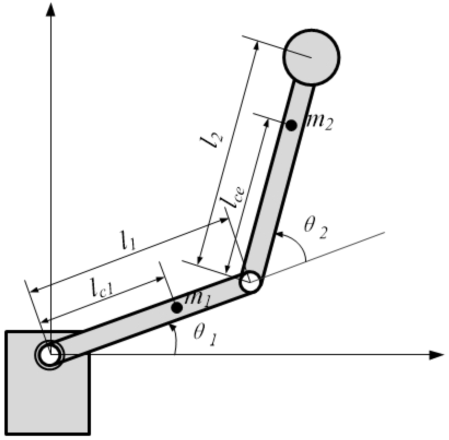
This study aims to verify the effectiveness of the proposed robot arm control method through simulations conducted on a two-degree-of-freedom robot arm, as illustrated in Figure 1. The experimental objectives of this paper consist of two aspects: first, to investigate the performance of the FCC under different $\mathit{f}$ values, and second, to validate the advantages and disadvantages of the TDE, NTSM, and FCC under different frictional force disturbances. Therefore, we conducted three sets of comparative experiments to evaluate the performance of three algorithms under three different conditions: no friction, normal friction disturbance, and significant friction disturbance.

To facilitate the simulation, the dynamic model of the robot arm system is presented in Equation (1). Detailed information on the model is presented below:

$$\mathit{M}(\mathit{\theta })=\left[\begin{array}{cc}\alpha +2\delta cos\left({\theta }_2\right)+2\eta sin\left({\theta }_2\right)& \beta +\delta cos\left({\theta }_2\right)+\eta sin\left({\theta }_2\right)\\ \beta +\delta cos\left({\theta }_2\right)+\eta sin\left({\theta }_2\right)& \beta \end{array}\right]$$

(38)

$$\mathit{C}(\mathit{\theta },\dot{\mathit{\theta }})=\left[\begin{array}{cc}\left[-2\delta sin\left({\theta }_2\right)+2\eta cos\left({\theta }_2\right)\right]{\dot{\theta }}_2& \left[-\delta sin\left({\theta }_2\right)+\eta cos\left({\theta }_2\right)\right]{\dot{\theta }}_2\\ \left[\delta sin\left({\theta }_2\right)-\eta cos\left({\theta }_2\right)\right]{\dot{\theta }}_1& 0\end{array}\right]$$

(39)

$$\mathit{G}(\mathit{\theta })=\left[\begin{array}{c}\delta e_{2}cos\left({\theta }_1+{\theta }_2\right)+\eta e_{2}sin\left({\theta }_1+{\theta }_2\right)+\left(\alpha -\beta +e_1\right)e_{2}cos\left({\theta }_1\right)\\ \delta e_{2}cos\left({\theta }_1+{\theta }_2\right)+\eta e_{2}sin\left({\theta }_1+{\theta }_2\right)\end{array}\right]$$

(40)

Friction severely affects the control performance of robot systems. Therefore, we select the friction term as follows:

$$\mathit{F}(\mathit{\theta },\dot{\mathit{\theta }})=\left[\begin{array}{c}{F}_{v1}{\dot{\theta }}_1+F_{c1}sgn\left({\dot{\theta }}_1\right)\\ F_{v2}{\dot{\theta }}_2+F_{c2}sgn\left({\dot{\theta }}_2\right)\end{array}\right]$$

(41)

where $\alpha =I_1+m_1{l}_{c1}^2+I_e+m_e{l}_{ce}^2+m_e{l}_1^2,\beta =I_e+m_e{l}_{ce}^2,\delta =m_e{l}_1{l}_{ce}cos{\delta }_e,\eta =m_e{l}_1{l}_{ce}sin{\delta }_e$, $e_1=m_1{l}_1{l}_{c1}-I_1-m_1{l}_1^2, e_2=g/l_1$; m₁ denotes the mass of first link; $l_{cl}$ is the distance between the mass center of the first link and the first joint; $I_l$ is the moment of inertia of the first link; $m_e$ is the mass of second link with payload; $l_{ce}$ is the distance between the mass center of second link and the second joint; $I_e$ is the moment of inertia of the second link; ${\delta }_e$ is the angle relative to the original second link. The physical parameters of the robot manipulator are shown in

Table 1. The physical parameters of the robot manipulator.

Indices	${\mathit{l}}_1$	${\mathit{l}}_2$	${\mathit{l}}_{\mathit{c}1}$	${\mathit{l}}_{\mathit{c}\mathit{e}}$	${\mathit{I}}_1$	${\mathit{I}}_2$	${\mathit{m}}_1$	${\mathit{m}}_{\mathit{e}}$	${\mathit{\delta }}_{\mathit{e}}$
Value	1	1.2	0.5	1	0.083	0.4	1	3	0

.

This study compares the performance of three controllers in experiments:

1.

FCC: This is a time-delay estimation controller equipped with AFLS (as given in Equation (20)), which is thoroughly described in Section 3 of this paper. The control gains for this controller are set as follows: ${\overline{M}}_1=0.15$, ${\overline{M}}_2=0.15$, $k_{11}=10$, $k_{12}=10$, $k_{21}=70$, and $k_{22}=70$.

2.

NTSM: This technique is founded on the principles of TDE and sliding-mode control. It achieves the high-precision control of nonlinear dynamic systems by incorporating supplementary terms on the sliding surface. These terms help to mitigate the impacts that traditional sliding-mode control may generate, resulting in a superior level of control.

3.

TDC: A widely used control method for systems with a delay that effectively solves delay problems and improves the stability and precision of the control system.

To quantitatively evaluate the control performance of these three controllers, the study uses the maximum value, mean value, and standard deviation of the tracking error as performance indicators, marked as MAV, RMS, and Var, respectively, whose definitions can be found in [29]. In the three experiments, a normal level sinusoidal trajectory with sufficient smoothness is used, defined as ${\mathit{x}}_{1d}(t)={[2\sin (0.5\pi t);2\sin (0.5\pi t)]}^{T}rad$.

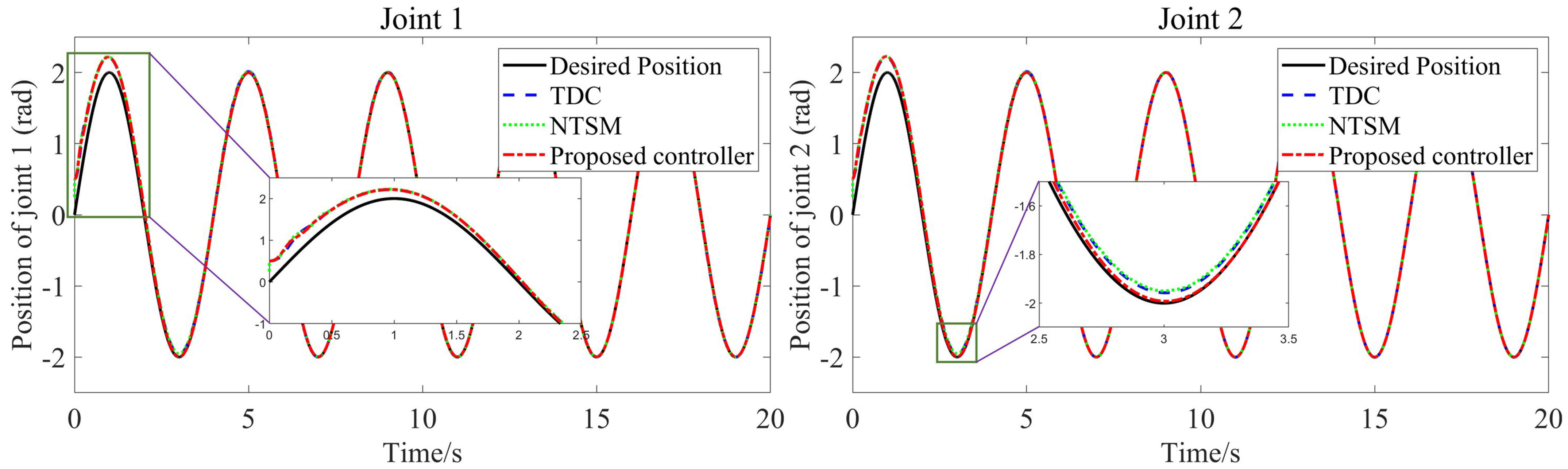
4.1. Comparative Experiment of Three Controllers under No-Friction Disturbance

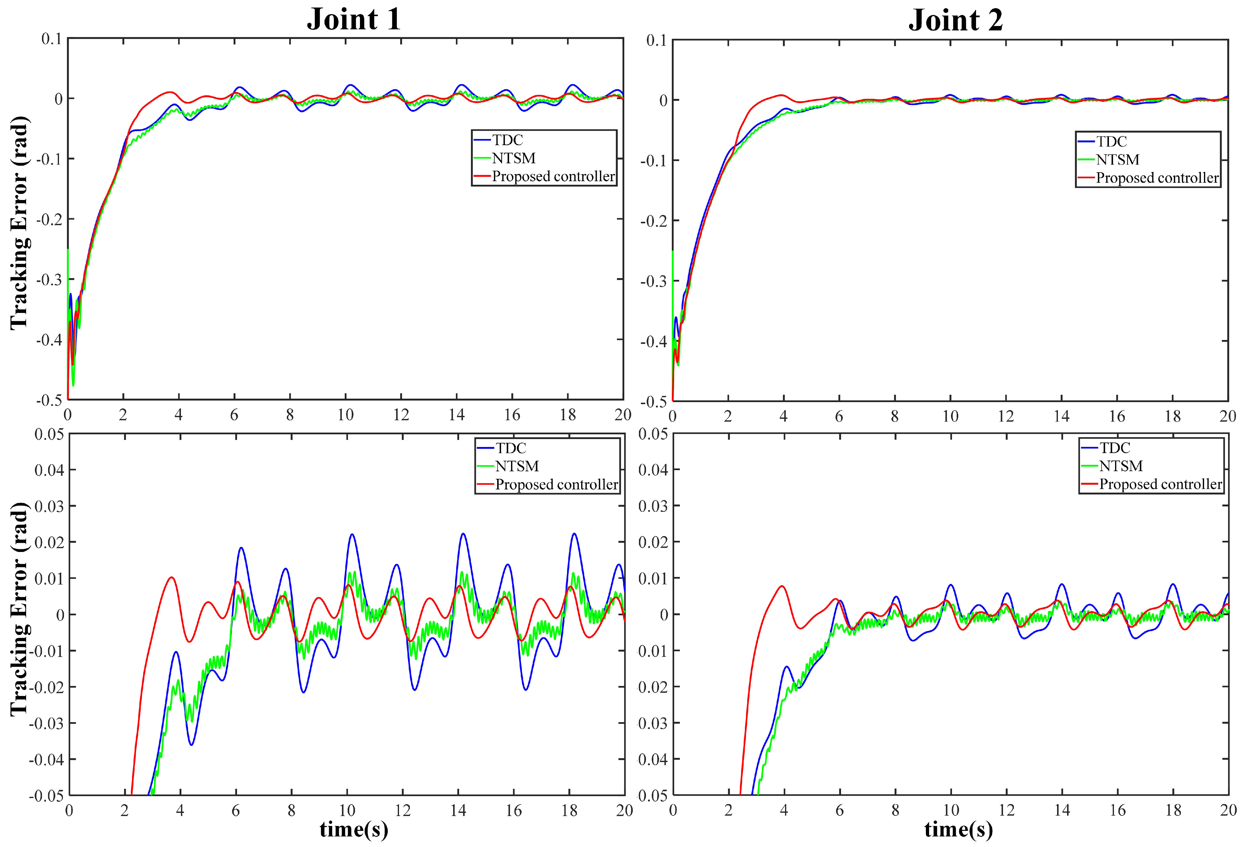
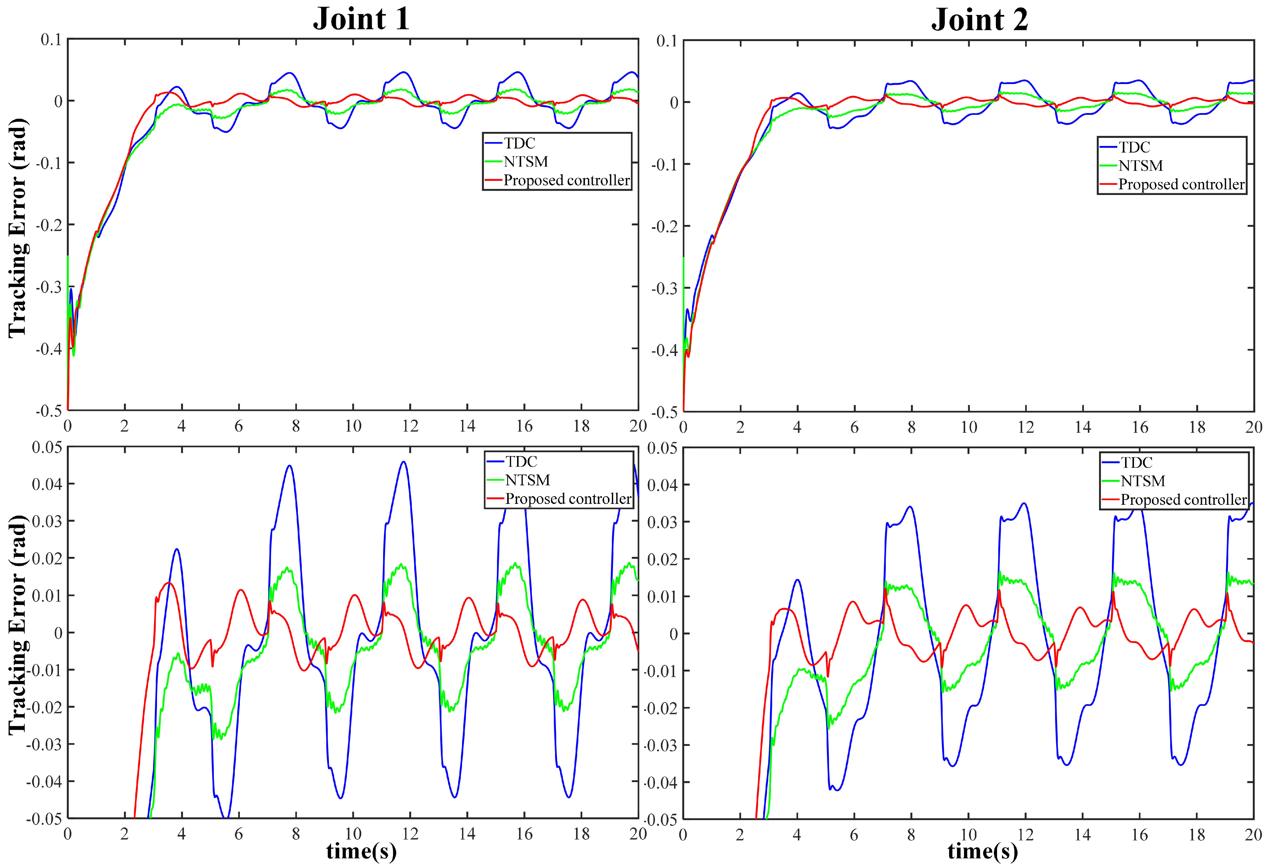
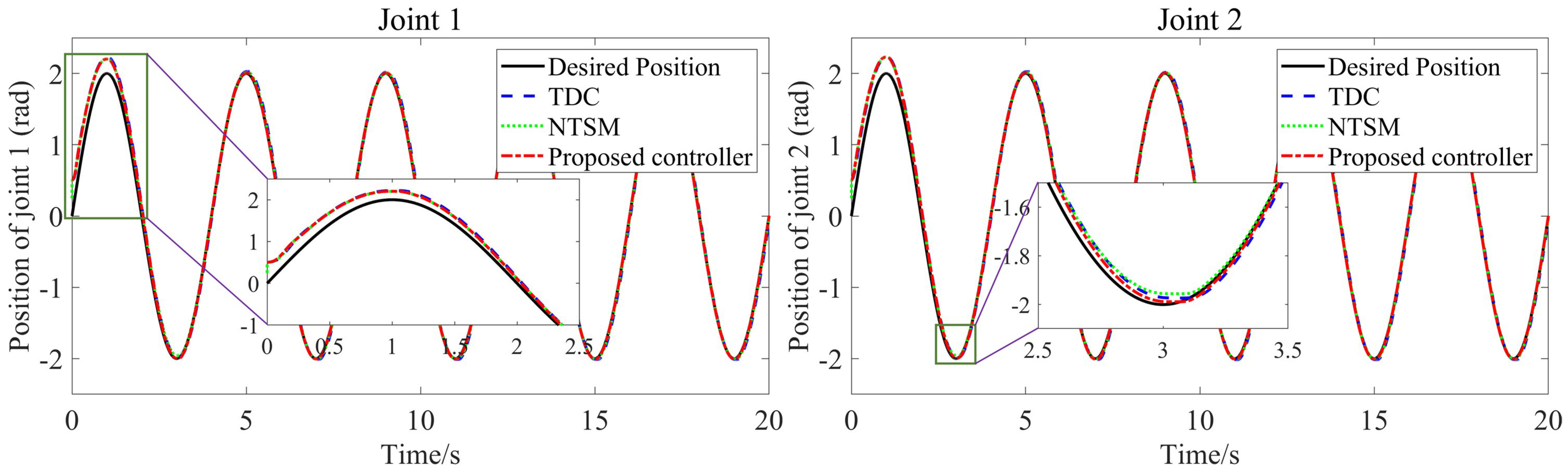
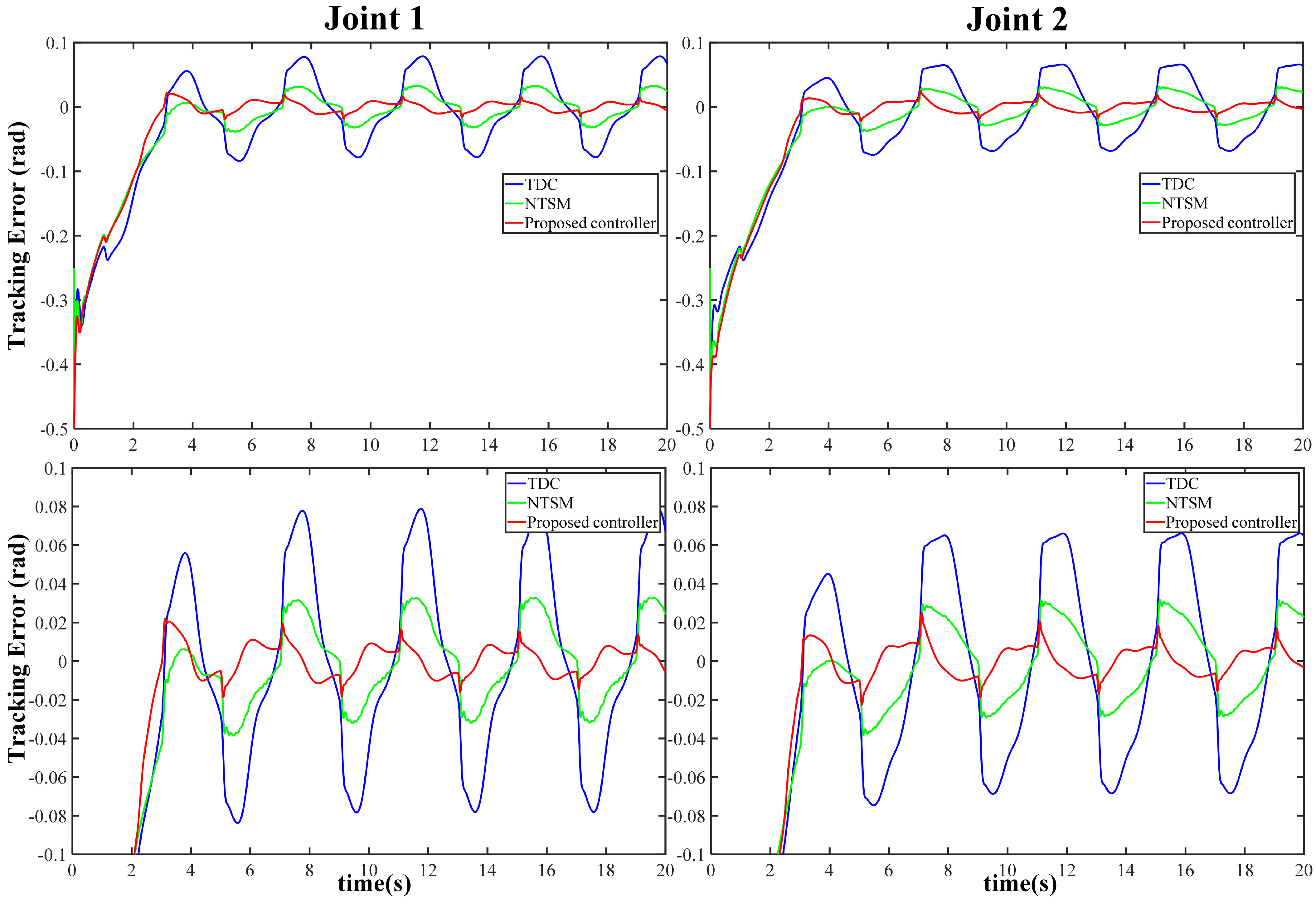
This section compares the simulation results of three algorithms at $F_{v1}=0$, $F_{c1}=0$, $F_{v2}=0$, and $F_{c2}=0$, as presented in Figure 2, Figure 3, Figure 4 and Figure 5. The FCC achieves maximum tracking errors of approximately $0.01$ rad and $0.005$ rad for joint 1 and joint 2, respectively. Compared to the TDC algorithm with linear error dynamics, the FCC exhibits smaller tracking errors. 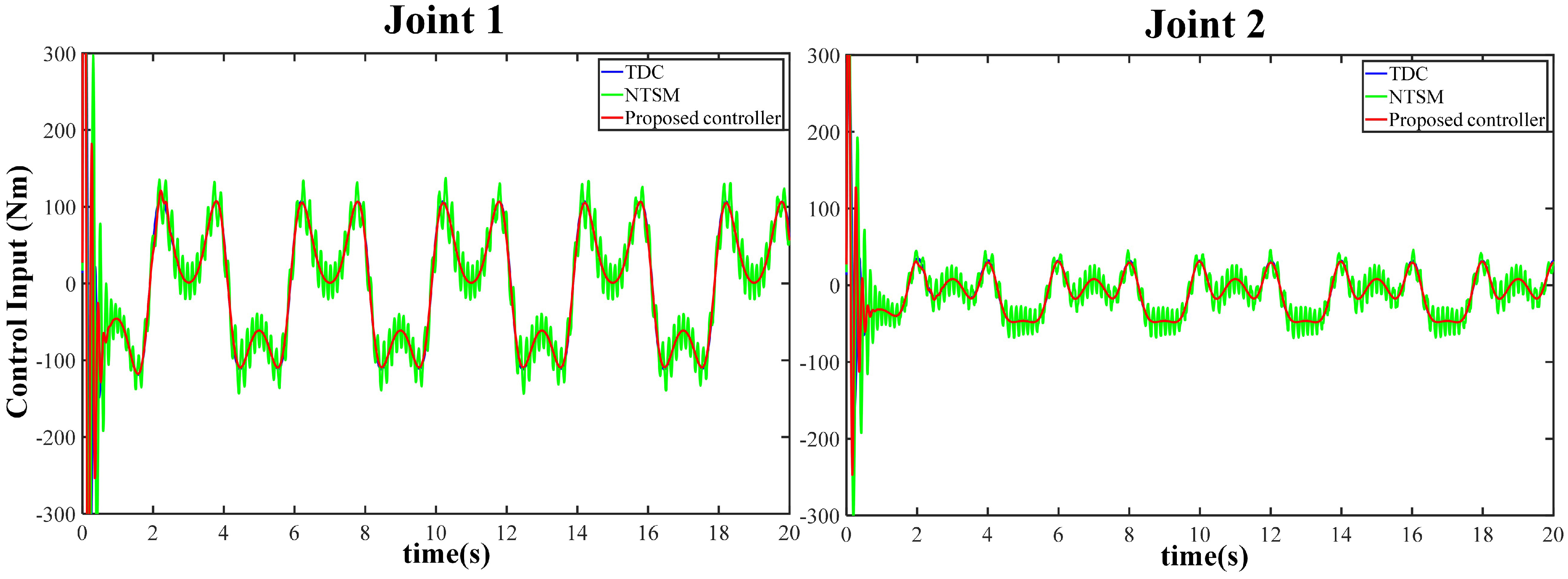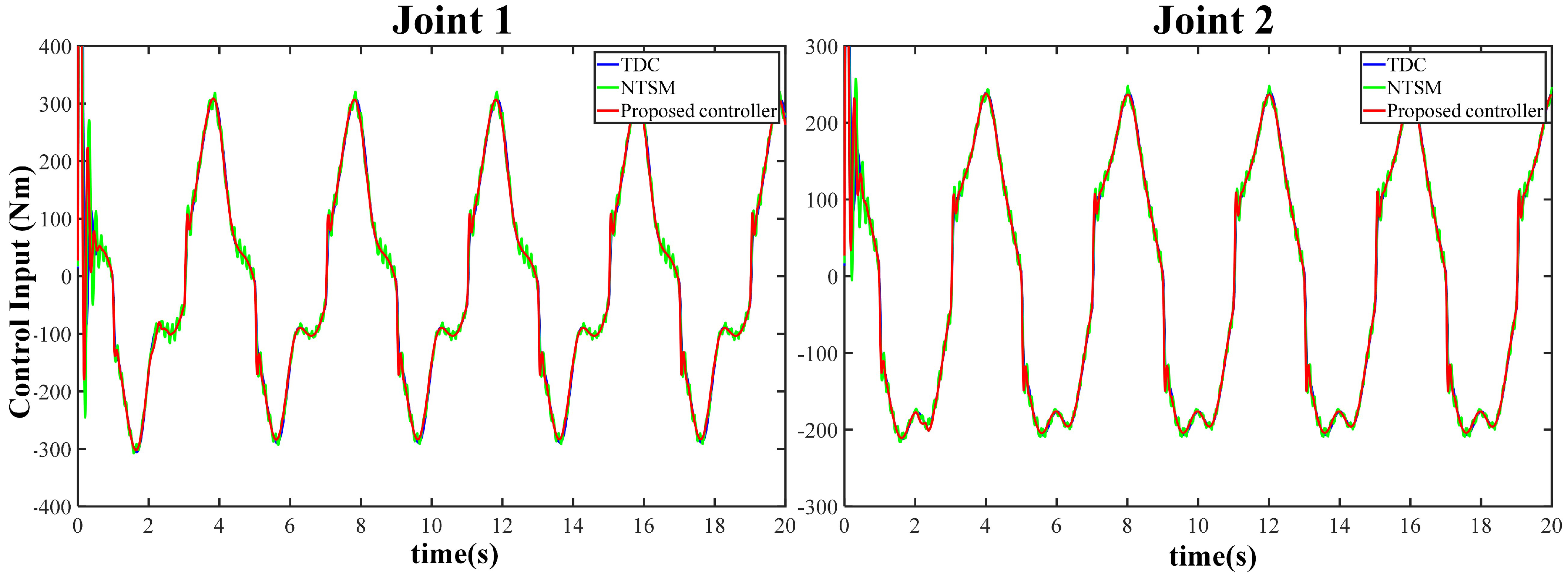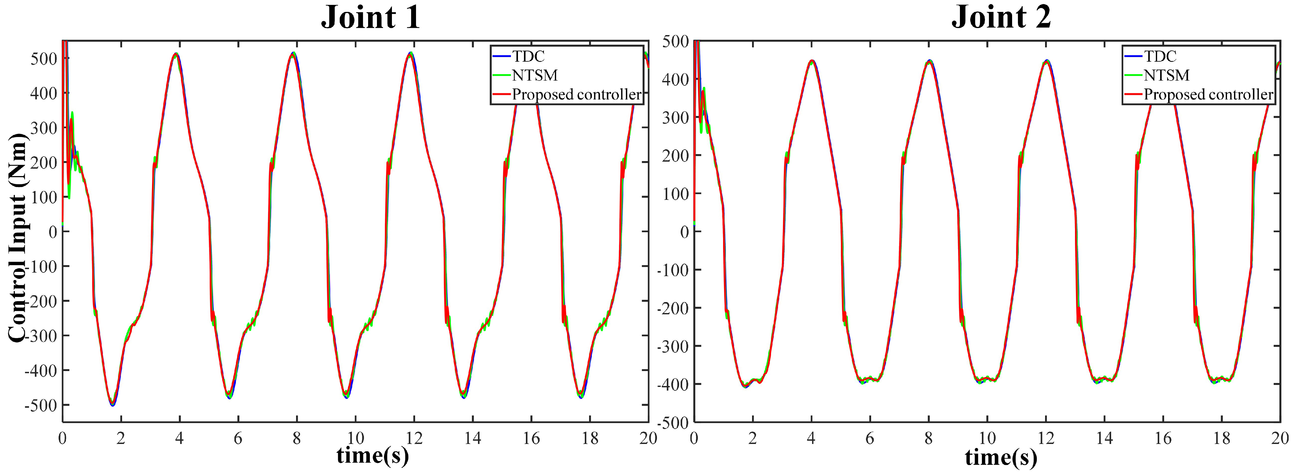Furthermore, Figure 4 demonstrates that there is no jitter in the control inputs of the two joints.

As illustrated in Figure 2, Figure 3, Figure 4 and Figure 5, the TDC algorithm effectively eliminates uncertainties and exhibits good tracking performance. Building upon this, the NTSM algorithm achieves high-precision tracking while also avoiding control jitter. Additionally, the FCC is proposed in this paper to achieve high-precision anti-interference control. In contrast to the TDC and NTSM algorithms, the FCC not only eliminates uncertainties but also achieves excellent tracking performance in the presence of frictional force interference.

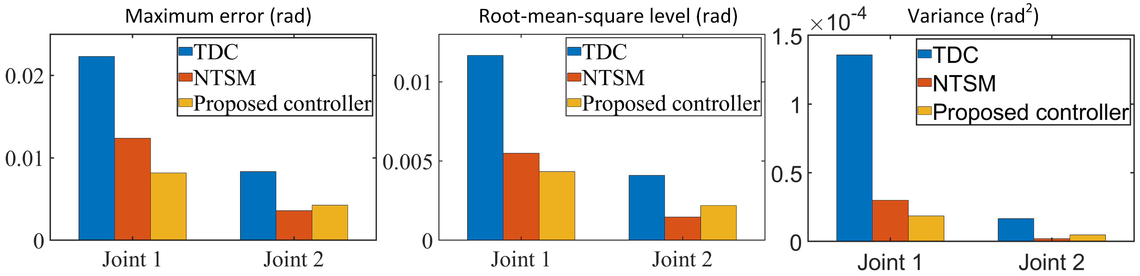
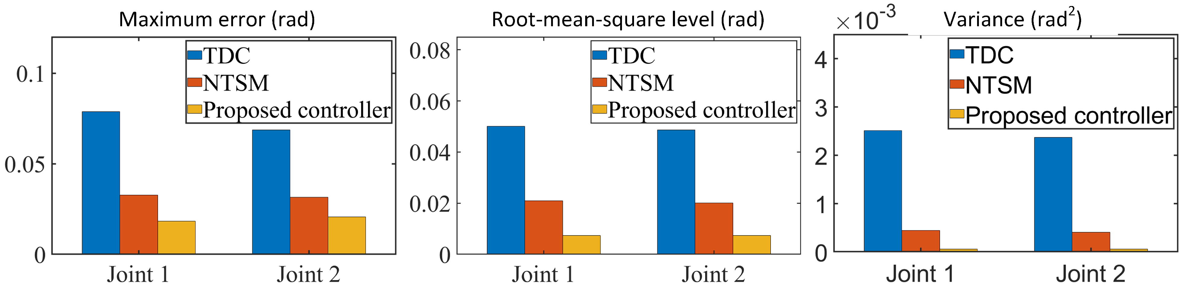
Figure 5 demonstrates the FCC’s outstanding tracking performance without frictional interference. The variance data in Figure 5 shows that the TDC controller’s tracking performance on joint 1 and joint 2 improved by 86.198% and 71.286%, respectively, after adding AFLS.

Remark 4. 

The variance of motion error in a robotic arm is a crucial metric for assessing its performance, enhancing control systems, optimizing motion trajectory planning, and predicting motion trajectories. To enhance the performance of a robotic arm, this study analyzes its errors by calculating variance and utilizes it as a reference point to gauge the extent of performance enhancement. For instance, on joint 1, the variance of TDC is $1.3575\times {10}^{-4}$, and the variance of FCC is $1.875\times {10}^{-5}$. As a result of this calculation, it is determined that the performance of joint 1 has been enhanced by 86.198%. It is important to note that all performance improvement ratios in this study are based on variance calculations.

4.2. Comparative Experiment of Three Controllers under Normal Friction Disturbance

To evaluate the high-precision tracking performance of the proposed algorithm, a certain amount of nonlinear friction disturbance was introduced to the system in this section by setting $F_{v1}=50$, $F_{c1}=50$, $F_{v2}=50$, and $F_{c2}=50$. Under these conditions, unmodeled nonlinear friction was identified as the primary source of disturbance and was used to test the robustness of the proposed FCC.

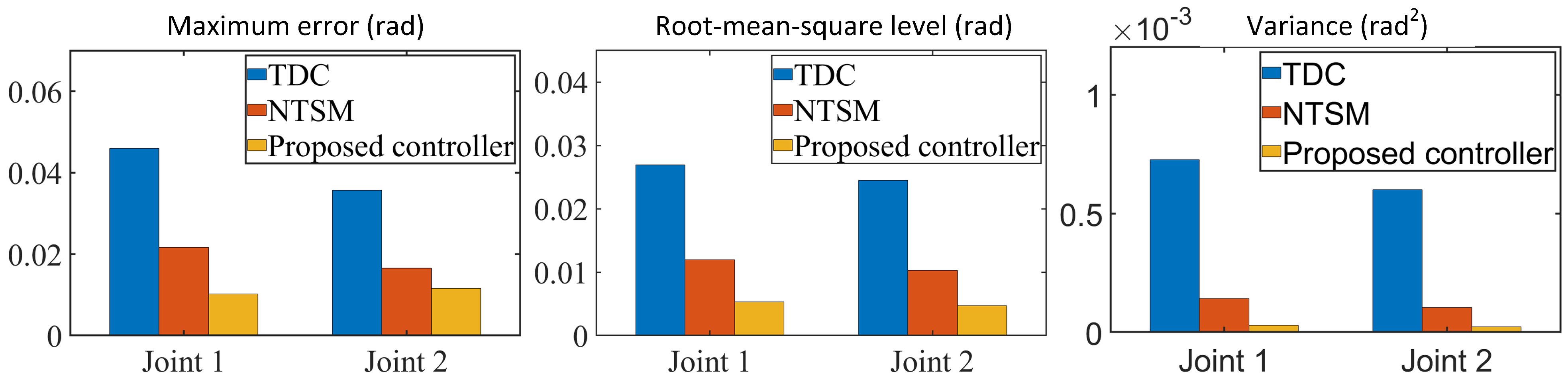
The simulation results presented in Figure 6 demonstrate that the FCC can accurately track the desired motion trajectory of the load. Figure 7 displays the tracking errors of the three controllers, indicating that the proposed FCC achieved the best tracking performance among the three controllers. The AFLS compensation mechanism resulted in better tracking performance than the NTSM. Figure 8 shows the control input voltage of the FCC, which is both smooth and limited. The performance indicators of the last three cycles are summarized in Figure 9. In the presence of normal friction disturbance, the FCC exhibited excellent anti-interference performance in the three indicators of MAV, RMS, and Var, which is the best among the three controllers. This is attributed to the faster convergence efficiency and high robustness of AFLS. Based on the variance shown in Figure 9, it is evident that the addition of AFLS improved the performance of TDC by 96.105% and 96.376% in joint 1 and joint 2, respectively.

4.3. Comparative Experiment of Three Controllers under Significant Frictional Disturbance

In this section’s three comparative experiments, a significant amount of frictional disturbance was introduced by setting $F_{v1}=100$, $F_{c1}=100$, $F_{v2}=100$, and $F_{c2}=100$.

The tracking trajectories and tracking errors of the three controllers are presented in Figure 10 and Figure 11. Figure 12 illustrates the control input voltage of the three controllers, indicating that their input voltage remains smooth and constrained. Figure 13 summarizes the performance indicators for the last three cycles, with TDC demonstrating the worst tracking performance due to its low robustness to nonlinear friction disturbance. In contrast, the FCC delivers the best performance in all performance indicators. Specifically, according to the variance shown in Figure 9, the addition of AFLS improves TDC performance by 97.885% and 97.712% for joint 1 and joint 2, respectively. The numerical experimental results reveal that, compared with the other two controllers, the proposed FCC delivers the best tracking performance in both transient and steady-state aspects.

We conducted a series of comparative experiments to verify the effectiveness and fast convergence of the FCC under various levels of frictional disturbances. The results showed that the proposed control algorithm exhibited excellent position-tracking performance. As the disturbance increased, the performance of FCC became increasingly superior, confirming the superiority and effectiveness of AFLS in terms of disturbance rejection. Therefore, the FCC not only possesses the fast convergence and efficiency of the TDC algorithm but also has the high disturbance-rejection capability and faster convergence rate of the AFLS algorithm. This further confirms the feasibility and effectiveness of the FCC in practical control applications.

4.4. Further Analysis of Error for Three Algorithms

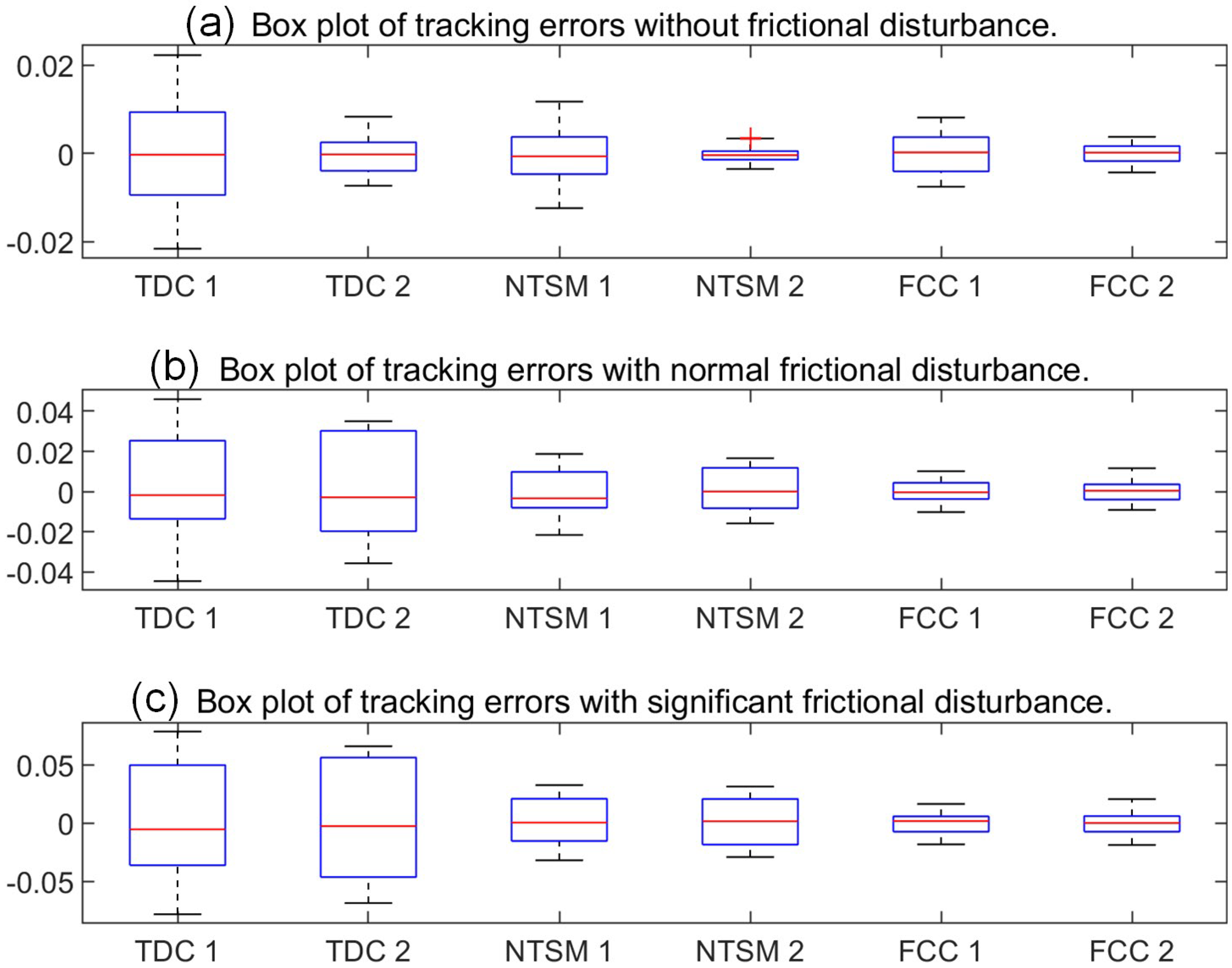
In this study, we analyzed the kinematic errors of three algorithms (TDC, NTSM, and FCC) applied to two joints of a robotic arm, using 20,000 samples. Box plots were used to display the data distribution and evaluate algorithm performance.

Figure 14 illustrates the distribution of kinematic errors in the robotic arm, with the x-axis indicating the joints and the y-axis indicating error values. Each box represents the error distribution of a joint, with the upper and lower boundaries indicating the upper and lower quartiles (Q3 and Q1), the middle line representing the median (Q2), and the internal line of the box indicating the mean. Outliers are shown outside the upper and lower limits of the box.

TDC 1 and TDC 2 represent the TDC algorithm applied to joints 1 and 2, respectively. Similarly, NTSM 1, NTSM 2, FCC 1, and FCC 2 represent the NTSM and FCC algorithms applied to joints 1 and 2 of the robotic arm. From Figure 14, it is apparent that the TDC algorithm has the largest error distribution, with the greatest distance between the upper and lower limits, but there are no outliers. The error distribution of the NTSM algorithm is relatively stable, with a lower height of the box and a smaller distance between the upper and lower limits, except for an outlier in NTSM 2. The error distribution of the FCC algorithm is the most stable, with the lowest average height of the box and the smallest distance between the upper and lower limits, and there are no outliers.

The box plot indicates that the FCC algorithm has smaller and more evenly distributed kinematic errors in each joint of the robotic arm, indicating superior tracking performance. Therefore, the FCC algorithm proposed in this study is an effective algorithm for controlling robotic arms.

5. Conclusions

In this paper, we propose a novel friction compensation controller (FCC) that integrates time delay estimation (TDE) and an adaptive fuzzy logic system (AFLS). The FCC method utilizes the TDE technique to eliminate and estimate the unknown dynamic functions of the system and incorporates an element for injecting expected error dynamics and an AFLS as the third element to handle strong nonlinearity and TDE errors. Additionally, an adaptive rule is designed to update the parameters of the fuzzy logic system online, improving the performance of the controller. Compared to existing TDC methods, the proposed method effectively suppresses TDE errors and provides a faster convergence rate. Moreover, the controller in this paper does not require complex offline parameter identification or precomputed models but can be implemented directly online, making it more suitable for practical systems.

Numerical experiments demonstrate that the proposed friction compensation control algorithm has fast convergence, high efficiency, and strong anti-interference capability, and achieves excellent position-tracking performance even under a large amount of nonlinear interference. Specifically, the addition of AFLS improves the performance of TDC by an average of 93.0623% and 88.125% for joint 1 and joint 2, respectively.

This study provides novel ideas and methods for the development of robot arm controllers and serves as a reference for the design of controllers in other industrial automation fields. The results indicate that the proposed FCC is a promising solution for controlling robotic systems with frictional effects and nonlinearities.

References

1. Izadbakhsh, A. An observer-based output tracking controller for electrically driven cooperative multiple manipulators with adaptive Bernstein-type approximator. Robotica 2022, 40, 2295–2319. [Google Scholar] [CrossRef]
2. Thomasson, O.; Battarra, M.; Erdoğan, G.; Laporte, G. Scheduling twin robots in a palletising problem. Int. J. Prod. Res. 2018, 56, 518–542. [Google Scholar] [CrossRef]
3. Sun, Y.; Wan, Y.; Ma, H.; Liang, X. Compensation control of hydraulic manipulator under pressure shock disturbance. Nonlinear Dyn. 2023, 1–17. [Google Scholar] [CrossRef]
4. Mir-Nasiri, N. Design, modelling and control of four-axis parallel robotic arm for assembly operations. Assem. Autom. 2004, 24, 365–369. [Google Scholar] [CrossRef]
5. Sabet, S.; Poursina, M. Computed torque control of fully-actuated nondeterministic multibody systems. Multibody Syst. Dyn. 2017, 41, 347–365. [Google Scholar] [CrossRef]
6. Jin, M.; Kang, S.H.; Chang, P.H. Robust compliant motion control of robot with nonlinear friction using time-delay estimation. IEEE Trans. Ind. Electron. 2008, 55, 258–269. [Google Scholar] [CrossRef]
7. Sun, Y.; Wan, Y.; Ma, H.; Liang, X. Workspace Description and Evaluation of Master-Slave Dual Hydraulic Manipulators. Actuators 2023, 12, 9. [Google Scholar] [CrossRef]
8. Cio, Y.S.L.K.; Raison, M.; Menard, C.L.; Achiche, S. Proof of concept of an assistive robotic arm control using artificial stereovision and eye-tracking. IEEE Trans. Neural Syst. Rehabil. Eng. 2019, 27, 2344–2352. [Google Scholar] [CrossRef]
9. Lee, J.; Deshpande, N.; Caldwell, D.G.; Mattos, L.S. Microscale precision control of a computer-assisted transoral laser microsurgery system. IEEE/ASME Trans. Mechatron. 2020, 25, 604–615. [Google Scholar] [CrossRef]
10. Chen, C.; Liu, Z.; Zhang, Y.; Xie, S. Coordinated motion/force control of multiarm robot with unknown sensor nonlinearity and manipulated object’s uncertainty. IEEE Trans. Syst. Man Cybern. Syst. 2016, 47, 1123–1134. [Google Scholar] [CrossRef]
11. Zhu, Y.; Qiao, J.; Zhang, Y.; Guo, L. High-precision trajectory tracking control for space manipulator with neutral uncertainty and deadzone nonlinearity. IEEE Trans. Control Syst. Technol. 2018, 27, 2254–2262. [Google Scholar] [CrossRef]
12. Zhang, A.; Ma, S.; Li, B.; Wang, M.; Guo, X.; Wang, Y. Adaptive controller design for underwater snake robot with unmatched uncertainties. Sci. China Inf. Sci. 2016, 59, 1–15. [Google Scholar] [CrossRef]
13. Hsia, T.S. A new technique for robust control of servo systems. IEEE Trans. Ind. Electron. 1989, 36, 1–7. [Google Scholar] [CrossRef]
14. Hsia, T.S.; Lasky, T.A.; Guo, Z. Robust independent joint controller design for industrial robot manipulators. IEEE Trans. Ind. Electron. 1991, 38, 21–25. [Google Scholar] [CrossRef]
15. Kali, Y.; Saad, M.; Benjelloun, K.; Khairallah, C. Super-twisting algorithm with time delay estimation for uncertain robot manipulators. Nonlinear Dyn. 2018, 93, 557–569. [Google Scholar] [CrossRef]
16. Ahmed, S.; Wang, H.; Tian, Y. Adaptive high-order terminal sliding mode control based on time delay estimation for the robotic manipulators with backlash hysteresis. IEEE Trans. Syst. Man Cybern. Syst. 2019, 51, 1128–1137. [Google Scholar] [CrossRef]
17. Van, M.; Ge, S.S.; Ren, H. Finite time fault tolerant control for robot manipulators using time delay estimation and continuous nonsingular fast terminal sliding mode control. IEEE Trans. Cybern. 2016, 47, 1681–1693. [Google Scholar] [CrossRef]
18. Jin, M.; Lee, J.; Ahn, K.K. Continuous nonsingular terminal sliding-mode control of shape memory alloy actuators using time delay estimation. IEEE/ASME Trans. Mechatron. 2014, 20, 899–909. [Google Scholar] [CrossRef]
19. Lee, J.; Chang, P.H.; Jamisola, R.S. Relative impedance control for dual-arm robots performing asymmetric bimanual tasks. IEEE Trans. Ind. Electron. 2013, 61, 3786–3796. [Google Scholar] [CrossRef]
20. Liang, X.; Wan, Y.; Zhang, C.; Kou, Y.; Xin, Q.; Yi, W. Robust position control of hydraulic manipulators using time delay estimation and nonsingular fast terminal sliding mode. Proc. Inst. Mech. Eng. Part I J. Syst. Control Eng. 2018, 232, 50–61. [Google Scholar] [CrossRef]
21. Geng, J.; Sheng, Y.; Liu, X. Time-varying nonsingular terminal sliding mode control for robot manipulators. Trans. Inst. Meas. Control 2014, 36, 604–617. [Google Scholar] [CrossRef]
22. Jin, M.; Kang, S.H.; Chang, P.H.; Lee, J. Robust control of robot manipulators using inclusive and enhanced time delay control. IEEE/ASME Trans. Mechatron. 2017, 22, 2141–2152. [Google Scholar] [CrossRef]
23. Adhikary, N.; Mahanta, C. Sliding mode control of position commanded robot manipulators. Control Eng. Pract. 2018, 81, 183–198. [Google Scholar] [CrossRef]
24. Lee, H.J.; Lee, J.J. Time delay control of a shape memory alloy actuator. Smart Mater. Struct. 2004, 13, 227. [Google Scholar] [CrossRef]
25. Cho, S.J.; Jin, M.; Kuc, T.Y.; Lee, J.S. Stability guaranteed auto-tuning algorithm of a time-delay controller using a modified Nussbaum function. Int. J. Control 2014, 87, 1926–1935. [Google Scholar] [CrossRef]
26. Jin, F.; Qiu, T. Adaptive time delay estimation based on the maximum correntropy criterion. Digit. Signal Process. 2019, 88, 23–32. [Google Scholar] [CrossRef]
27. Bae, H.J.; Jin, M.; Suh, J.; Lee, J.Y.; Chang, P.H.; Ahn, D.s. Control of robot manipulators using time-delay estimation and fuzzy logic systems. J. Electr. Eng. Technol. 2017, 12, 1271–1279. [Google Scholar] [CrossRef]
28. Arimoto, S.; Kawamura, S.; Miyazaki, F.; Tamaki, S. Learning control theory for dynamical systems. In Proceedings of the 1985 24th IEEE Conference on Decision and Control, Fort Lauderdale, FL, USA, 11–13 December 1985; pp. 1375–1380. [Google Scholar]
29. Yao, J.; Deng, W.; Jiao, Z. Adaptive control of hydraulic actuators with LuGre model-based friction compensation. IEEE Trans. Ind. Electron. 2015, 62, 6469–6477. [Google Scholar] [CrossRef]
Figure 1. Diagram of two-DOF robot manipulator.
Actuators 12 00184 g001
Figure 2. Position-tracking curves for the three controllers under no-friction disturbance.
Actuators 12 00184 g002
Figure 3. Tracking-error curves of the three controllers under no-friction disturbance.
Actuators 12 00184 g003
Figure 4. The control input voltage curves of the three controllers under no-friction disturbance.
Actuators 12 00184 g004
Figure 5. Performance indices evaluation during the last three cycles under no-friction disturbance.
Actuators 12 00184 g005
Figure 6. Position-tracking curves for the three controllers under normal friction disturbance.
Actuators 12 00184 g006
Figure 7. Tracking-error curves of the three controllers under normal friction disturbance.
Actuators 12 00184 g007
Figure 8. The control input voltage curves of the three controllers under normal friction disturbance.
Actuators 12 00184 g008
Figure 9. Performance indices evaluation during the last three cycles under normal friction disturbance.
Actuators 12 00184 g009
Figure 10. Position-tracking curves for the three controllers under significant frictional disturbance.
Actuators 12 00184 g010
Figure 11. Tracking-error curves of the three controllers under significant frictional disturbance.
Actuators 12 00184 g011
Figure 12. The control input voltage curves of the three controllers under significant frictional disturbance.
Actuators 12 00184 g012
Figure 13. Performance indices evaluation during the last three cycles under significant frictional disturbance.
Actuators 12 00184 g013
Figure 14. Tracking-error curves of the three controllers under significant frictional disturbance.
Actuators 12 00184 g014