Modeling and Theoretical Analysis of Zero-Flowrate-Switching Control Method for a Dynamic Load System to Reduce Switching Power Loss of Control Valves

Abstract

Valve switching is one of the most important power losses in digital hydraulics. In this paper, a dynamic Zero-Flowrate-Switching (ZFS) control method is developed for hydraulic/pneumatic systems. The proposed control strategy is to actively reduce the flowrate passing through the valve to zero before switching off the valve. To realize it, an accessory line, in which a RLC oscillator is applied to generate a sinusoidal flowrate, is allocated parallel to the main control line for flowrate regulation. The pressure, with high frequency and small amplitude wave outputs from a regular piston pump, is used to drive the RLC oscillator. To evaluate the performance of this strategy, mathematical models for switching power loss and pressure pulses are developed and characteristic analysis is conducted. The results show that the energy loss of the system when applying the dynamic ZFS controller is reduced to 16% compared to that of a normal hydraulic system without a dynamic ZFS controller; moreover, pressure pulses in a dynamic ZFS system are much more minor than those in a Hard-Switching system.

1. Introduction

Digital hydraulic systems, which apply a number of fast-switching valves switching at high frequencies [1,2,3,4,5,6], show higher theoretical efficiency and better controllability than traditional servo/proportional ones. In principle, applying fast switching valves in digital hydraulic systems could efficiently avoid energy consumptions that go over the valves. However, the response time of physical valves can only achieve between 1–2 ms; during a switching-off process, a certain switching power loss will be generated, since a pressure difference and flowrate exist before the valve is completely switched off. Moreover, when the valve is suddenly switched off, the fluid with a large kinetic energy will generate large pressure pulses, which lead to vibrations and noises and make the system less efficient and accurate [7].

In recent years, many works in digital hydraulics have been conducted to improve system efficiency and eliminate pressure pulses [8,9,10,11,12]. For example, the Fibonacci coding method is proposed to ease the pressure pulses by decreasing the quantity of digital valves switching at the same time compared to binary coding in a PCM method [8]. A flatness-based controller is designed for the Hydraulic Buck Converter (HBC), which aims to attenuate pressure ripples and oscillatory response [9]. In addition, Johnston et al. proposed some analytical models for a switched inertance hydraulic system in a four-port high-speed switching valve configuration [10,11,12]. These models provide promising ways to understand the characteristics of a four-port hydraulic system that includes a flowrate/pressure response. With these models, they analyzed the performance of a flow booster with a high-speed rotary valve, which is designed to minimum the pressure/flow loss through the valve orifice. They also proposed an active method for pressure pulsation cancellation by superimposing an anti-phase control signal. In [13] Y. Alexander C. and V. James D. proposed a soft-switching method in a switched inertance hydraulic circuit. In the proposed method, the flow that would otherwise be throttled across the transitioning valve is stored in a capacitive element and bypassed through check valves in parallel with the switching valves. This method aims to reduce the switching power loss caused by the overlap of the directional valves. In [14], a monotube was applied to absorb pressure shock.

The nature of control valves is to throttle flowrate and yield pressure pulses. All the research above was to passively improve system efficiency, while none of the studies focused on the reason for pressure pulses and energy consumption. In [15], we firstly proposed the concept of the Zero-Flowrate-Switching controller, which reduces energy loss by reducing the flowrate of the switcher to zero when it is time to shut off the switcher. In this way, it is possible to greatly depress pressure pulses and ultimately reduce energy consumption. The ZFS control method for hydraulic applications is inspired by electronic soft-switching techniques [16,17,18,19]. A resonant line is based on a RLC oscillator and assisted by other potential lines to achieve the purpose. A theoretical framework of a ZFS controller for a basic one-direction actuation system was mathematically modeled. In [15], the frequency and amplitude of the supply pressure were assumed as 50 Hz and 1 bar to validate the feasibility of the ZFS controller in a simple one-direction hydraulic line; however, there is a key problem in the application of the ZFS controller: a ZFS controller needs an AC supplier while the DC source is employed in hydraulic systems. To solve this problem, the authors figured out a new measuring method—the fiber brag measuring method—to measure the output pressures of an actual pump (Hydroleduc W12) [20,21]. In the following publication [22], we validated the feasibility of the output pressure waves of the actual pump as the supplier of a ZFS controller, and the result was positive. Additionally, we analyzed the characteristics of this ZFS controller in a double-direction hydraulic line. The results presented a 14.7% switching power loss compared to that of a Hard-Switching (HS) control system in a double-direction hydraulic system.

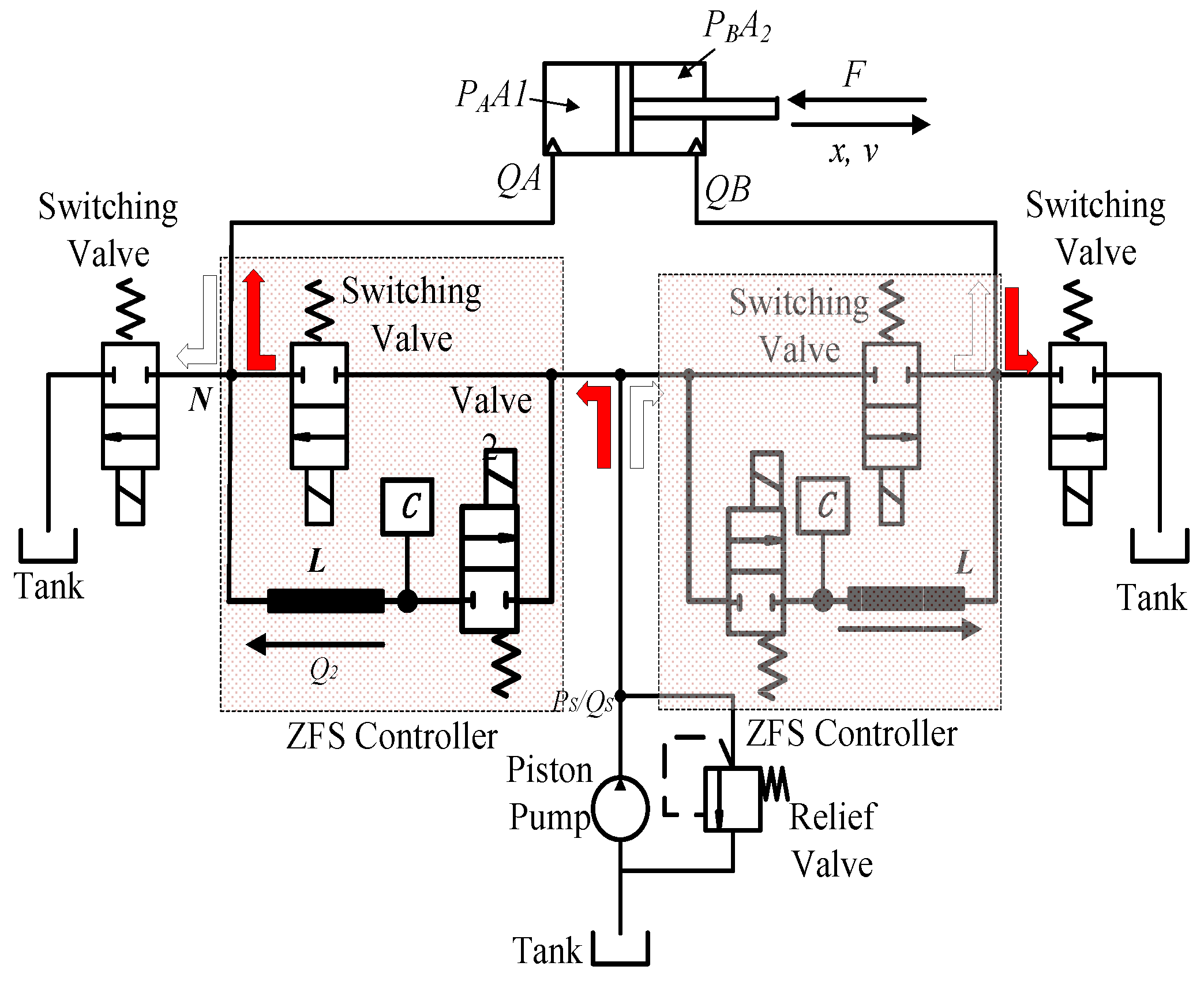
However, the characteristics of hydraulic systems are different from that of electronic counterparts. The performance is complex in the valve start-up process [23]. Many hydraulic problems should be resolved before a real hydraulic ZFS model is developed. Linear hydraulic components such as the inductance/capacitance should be investigated in a RLC resonator; unexpected hydraulic capacitance needs to be properly considered, since dynamic load forces have an impact on pressure/flowrate response and system capacitance. In this paper, a dynamic ZFS control method for a 4-port hydraulic system is proposed. In the dynamic ZFS controller presented in this paper, dynamic load forces are applied in the model; in the meantime, the impact of the dynamic load forces on the cylinder chamber pressures/flowrates and system capacitance is also considered in this advanced model.

The paper is organized as follows. The second section explains how the switching power loss and pressure pulses are generated in a switching system; the third section presents the schematic of a ZFS control system where two ZFS controllers are used for both extension and drawing back motions of the cylinder in a typical four-port switching system; the principle of a ZFS controller is introduced in this section; after that, mathematic models are built in Section 4; in Section 5, a dynamic load is modeled, cylinder capacitance is investigated, and the switching power loss and pressure pulses are also modeled. After that, simulation results are presented in Section 6. At the end of the paper comes the conclusions for this proposed hydraulic control method.

2. Statement of the Problems and Principle of the ZFS Control Method

2.1. Statement of the Problems

As presented in Figure 1, a typical digital hydraulic system actuates the hydraulic cylinder by several fast-switching valves. When the piston of the cylinder is extending, the fluid flows, as indicated by the red arrows; when extracting, the circuit works in the way presented by the white arrows.

When the cylinder is extending, the control line between the power unit and the cylinder is simplified, as Figure 2 shows. The power source P_S supplies the load (pressure P_A and flowrate Q_A) through a fast-switching valve. The fast-switching valve is powered by a PWM controller which actuates the valve to switch at a high frequency. Switching off the valve introduces switching power loss and pressure pulses which make the system response less smooth and less efficient. Moreover, it results in noises and vibrations that do harm to the system. Referring to the concept of the ZFS controller, this line is referred to as ‘a Hard-Switching (HS) Controller’.

2.1.1. Switching Power Loss

Theoretically, the fast-switching valve works only in ON and OFF states; the switching power loss is supposed to be zero. However, physical switching valves are not ideal ones. It is assumed that the flowrate-to-time is linear for the valve opening of valve 1 and valve 2, thus the orifice coefficient of the valve opening is

$$C_{orif}\left(t\right)=1-\frac{t-t_0}{T_s},$$

(1)

where t is time, t₀ is the initial moment to switch the valve and T_S is the switching time of the valve. During the switching process, both the flowrate and pressure difference are none-zero. The switching power loss for the switching valve in Figure 2 is derived as

$$E_{loss}={{\displaystyle \int }}_{t_0+NT}^{t+T_S+NT}{C}_{orif}{Q}_A\left(P_S-P_A\right)\mathrm{d}t,$$

(2)

where T is the time period of the pressure waves; N = 0, 1, 2, 3…; as presented in Figure 3, at the beginning of the switching-off process, P_S(t) − P_A(t) is small but the value of Q_A(t) is close to required flowrate; at the end of the switching-off process, P_S(t) − P_A(t) is equal to P_S(t), which is a large value, while Q(t) is small. A certain level of power loss is observed during this process.

As indicated in Equation (2), a high switching frequency f_PWM, large flowrate Q_A or pressure difference will give rise to switching power loss, which is a serious problem in the applications with high frequent switching, large system flowrate or large pressure difference.

2.1.2. Pressure Pulses

When the switching valve shuts off suddenly, the fluid energy before the valve fulfills

$$E_k=E_p+E_{loss},$$

(3)

where the kinetic energy E_k and the potential energy E_p [24] are

$$E_k=\frac{1}{2}\rho L_{pipe}A{v}_0^2,$$

(4)

$$E_p=\frac{1}{2}\frac{L_{pipe}A}{E}{P}_{pulse}^2,$$

(5)

where ρ is the density of hydraulic fluid; L_pipe is the length of the pipe between the pump and the valve; A is the area of the pipe; v₀ is the velocity of the fluid; E is the elastic bulk of the fluid and P_pulse is the peak value of the pressure pulses. According to Equations (3)–(5), the larger the flowrate is, the higher the pressure pulses are. Pressure pulses are normally found in systems with large flowrates.

2.2. Why the ZFS Control Method?

As stated above, systems with large flowrates can suffer both switching power loss and pressure pulses; reducing the flowrate before the pressure goes up to a certain level is a solution for both problems (shown in Figure 4). A Zero-Flowrate-Switching (ZFS) control method is a way to make the flowrate through the switching valve as small as possible during the switching-off process. In this way, it restrains pressure pulses and reduces switching power loss for high switching-frequency hydraulic systems.

2.3. The Principle of the ZFS Control Method

2.3.1. A ZFS Controller

In this paper, the ZFS control method is proposed to actively reduce switching power loss and restrain the pressure pulses for a typical four-port switching system—shown in Figure 1—to achieve a more efficient and smoother performance. The four-port switching hydraulic system controlled by the ZFS controllers is shown in Figure 5. The groups covered by red sheets are two ZFS controllers: one is to regulate extension motion and the other is for the drawing back of the cylinder. A ZFS controller includes a main control valve and a resonant line; the resonant line consists of a switching valve, a hydraulic inductance and a hydraulic capacitance.

The ZFS control method is to regulate the flowrate of the switching valve to zero right before the valve switches off. Figure 6 presents a hydraulic schematic of a ZFS controller. It consists of a main control line and a resonant line. The main control line is to supply the pressure and flowrate for the load. When it is about to close the main control line, it opens the resonant line, and then the flowrate of the resonant line starts to increase. Accordingly, the flowrate of the main control line falls down until it is zero. Then, the main control line is closed. This is the principle of a ZFS controller.

2.3.2. A Resonant Line

An electronic RLC resonator, shown in Figure 7a, consists of resistance, inductance and capacitance. When the inductance is equal to the capacitive reactance, the electronic flow will resonate with the excitation of an AC source.

In a hydraulic counterpart, the resonant line is composed of a fast-switching valve, hydraulic inductance and hydraulic capacitance (shown in Figure 7). The power supplier is a regular piston pump which outputs constant pressure with tiny amplitude waves.

$$P_S=P_{S0}+P_{Sa}\sin \omega t,$$

(6)

where P_S0 is the average value of the supplied pressure; P_Sa is the amplitude of the pressure waves and ω is the angular speed of the pressure waves. The term $P_{Sa}\sin \omega t$ is used to generate the sinusoidal resonant flowrate Q_res. When the RLC resonator works, the pressure waves distributed along the line are represented as

$$R{Q}_{res}\left(t\right)+L\frac{\mathrm{d}{Q}_{res}}{\mathrm{d}t}+\frac{1}{C}{{\displaystyle \int }}_0^t{Q}_{res}\left(t\right)\mathrm{d}t=P_{Sa}\sin \left(\omega t\right),$$

(7)

where Q_res is resonant flowrate and C is number for the hydraulic capacitance. For this case, the relationship between the pressure drop p and flowrate q of the valve is assumed to be linear

$$p=Rq,$$

(8)

Differentiating and dividing by L leads to the second order differential equation

$$\frac{{\mathrm{d}}^2{Q}_{res}\left(t\right)}{\mathrm{d}{t}^2}+\frac{R}{L}\frac{\mathrm{d}{Q}_{res}\left(t\right)}{\mathrm{d}t}+\frac{1}{LC}{Q}_{res}\left(t\right)=\frac{\omega P_s}{L}\sin \left(\omega t-\frac{\pi }{2}\right);$$

(9)

when

$$\omega ={\omega }_0=\frac{1}{\sqrt{LC}},$$

(10)

the output flowrate Q_res is derived as

$$Q_{res}\left(t\right)=\frac{P_{sa}}{R}$$

(11)

To make the ZFS controller work, Q_res fulfills

$$Q_{res}\left(t\right)>Q_{Smax},$$

(12)

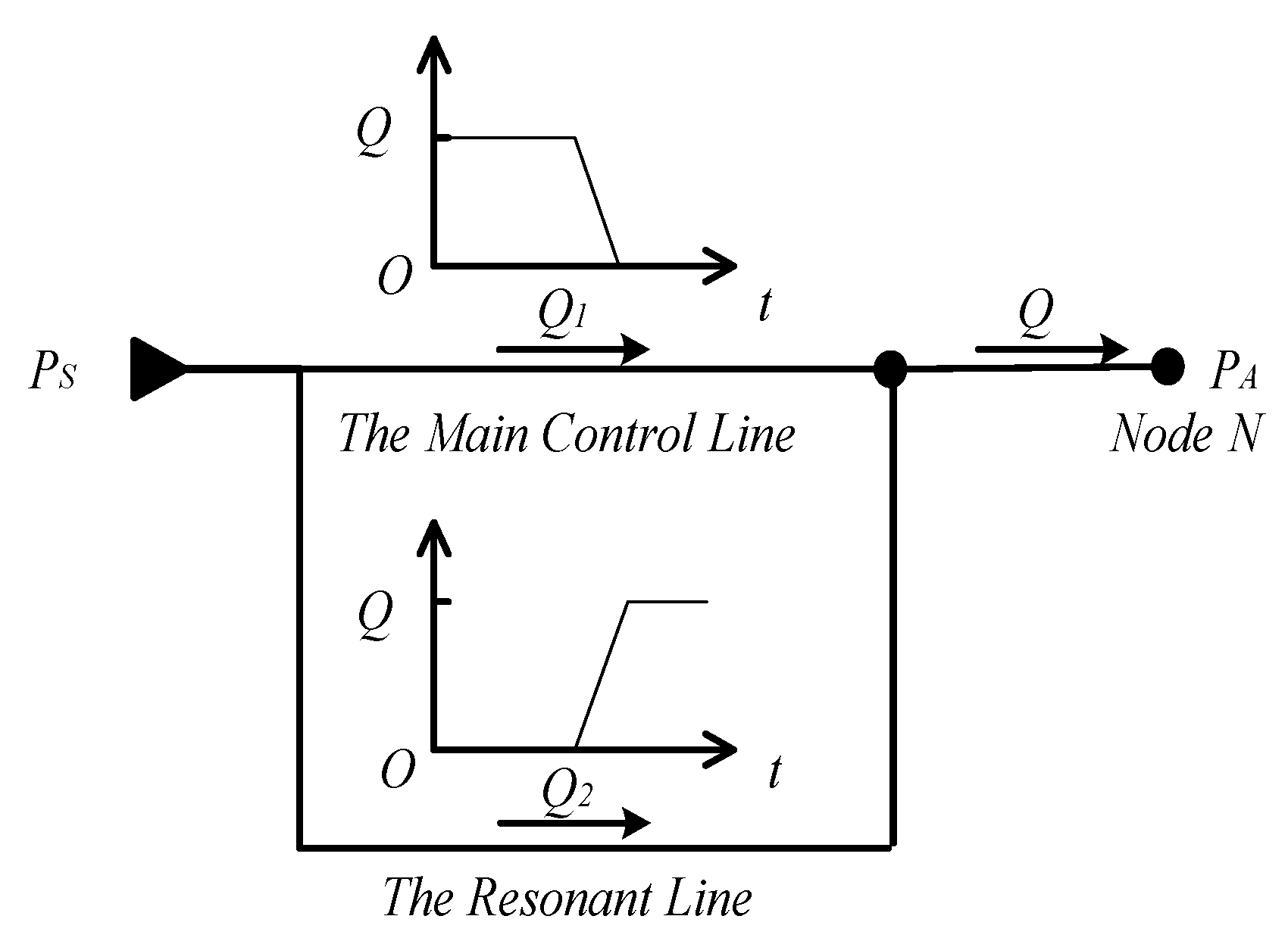
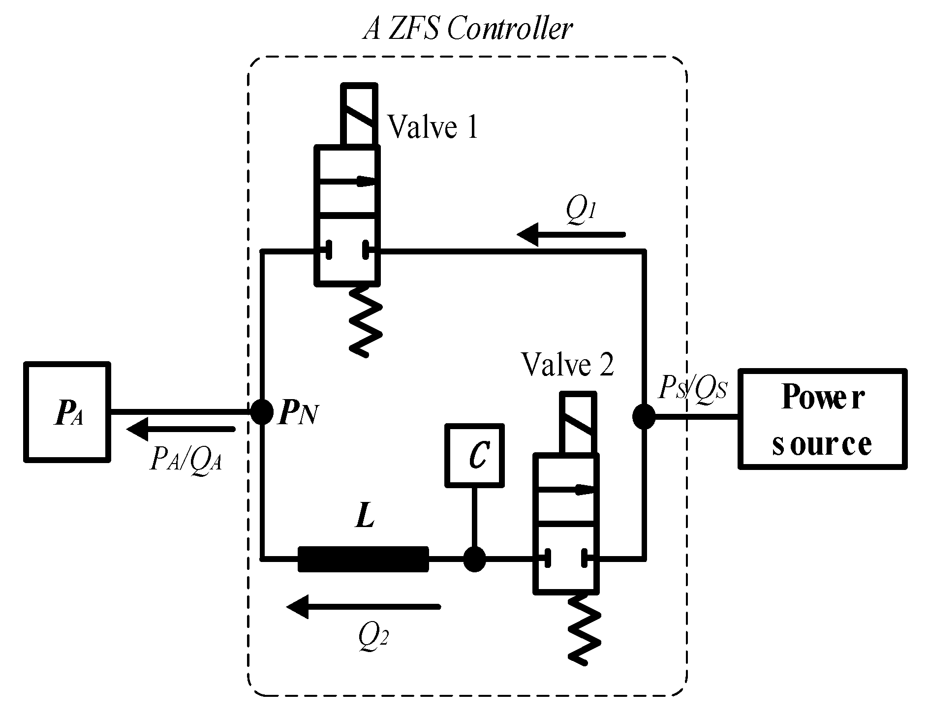
3. Mathematic Model of a ZFS Control System

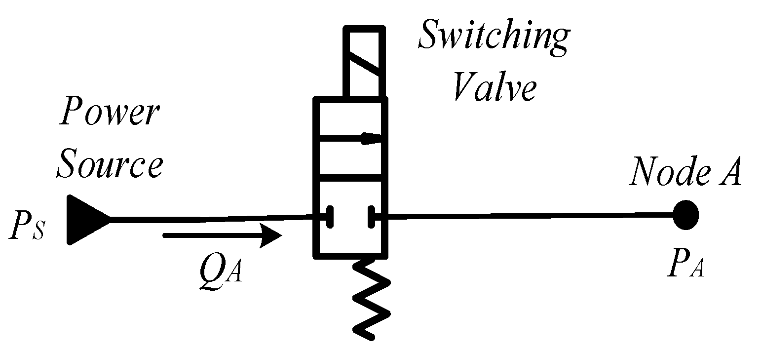
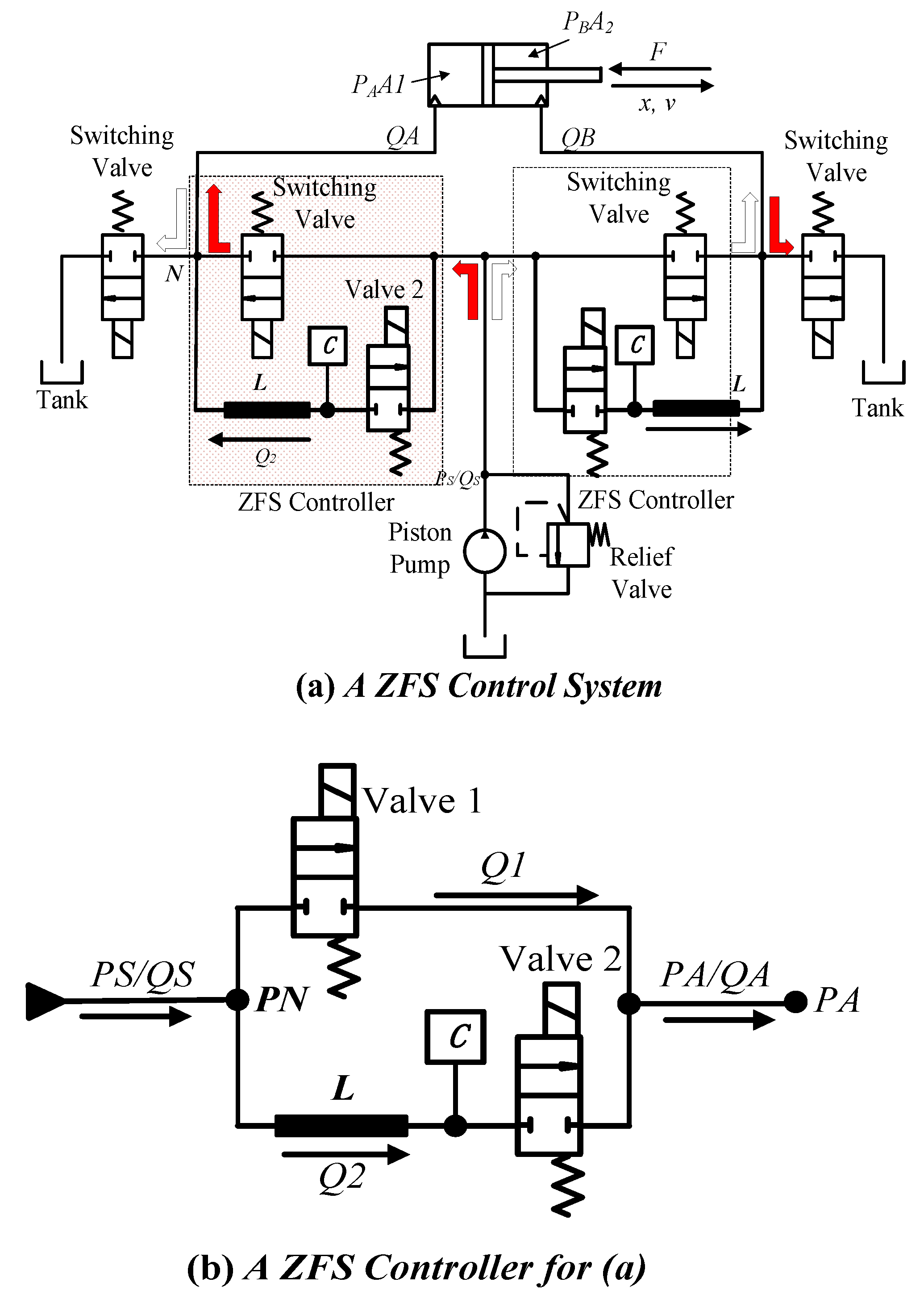
In this section, a ZFS control model with a dynamic load force will be introduced. In [20], the authors have proposed a basic ZFS model. As shown in Figure 8, valve 1 is the control valve which stays open when the control line (the line between power source and PA) is working. When the control line is required to stop, valve 1 will not switch off immediately; instead, the resonant line will start to participate in order to switch off the control line until the control line is ultimately switched off. There are four modes during the whole switching-off process: mode 1, mode 2, mode 3 and mode 4. The working principle for the four modes is explained in [20]; the related flowrates for each of the modes are presented in

Table 1. State matrix of the valves.

Operating Modes	Valve 1	Valve 2	Flowrate
Mode 1	ON	OFF	$$\begin{gathered} Q_1=Q_A \\ {Q}_2=0 \end{gathered}$$
Mode 2	ON	ON	$$\begin{gathered} Q_1=Q_{res}-Q_A \\ {Q}_2=Q_{res} \end{gathered}$$
Mode 3	OFF	ON	Stage 1: $$\begin{gathered} Q_1=-C_{orif}\left(Q_{res}-Q_A\right) \\ {Q}_2=Q_{res} \end{gathered}$$ Stage 2: $$\begin{gathered} Q_1=0 \\ {Q}_2=Q_A \end{gathered}$$ Stage 3: $$\begin{gathered} Q_1=0 \\ {Q}_2=Q_{Smax}+Q_{res} \end{gathered}$$
Mode 4	OFF	OFF	$Q_1=0; Q_2=0$

.

3.1. Dynamic Load of the ZFS Controller

Based on the model in Figure 8, the system characteristics with dynamic loads will be further discussed in this work. In the model described in Figure 8, the piston is moving with a constant velocity and varied load force, thus the input pressure of the cylinder is

$$P_A=\frac{P_B{A}_2+F}{A_1},$$

(13)

The tank pressure is zero, thus the pressure P_B can be regarded as the pressure difference across the valve, and is derived as follows

$$P_B=\frac{\rho }{2}{\left(\frac{Q_B}{C_q{A}_{valve}}\right)}^2,$$

(14)

$$Q_B=v{A}_2$$

(15)

where Cq is flow coefficient and ρ is the density of the fluid. Hence, P_A is derived as

$$P_A=\frac{A_2}{A_1}{\left(\frac{v{A}_2}{C{A}_{valve}}\right)}^2+\frac{F}{A_1},$$

(16)

3.2. Dynamic Capacitance of the Cylinder

In a ZFS controller, the resonant line generates flowrate waves to make the flowrate through the valves reduce to zero. Theoretically, the valve switches off at the zero-flowrate moment, and the power loss is thus zero. However, the switching-off moment of the valve cannot exactly match the zero-flowrate moment in a real hydraulic system. The error between the switching-off moment and the zero-flowrate moment will lead to some power loss. The larger the error is, the more the power loss is. Therefore, accurately simulating zero-flowrate moments is very important to improve system efficiency.

Normally, the input flowrate of a cylinder is calculated with the piston velocity timing and piston area. However, the capacitance of the input chamber of a cylinder has an influence on its flowrates. When the system load force is various, cylinder capacitance can be complex. To better simulate the input flowrate of the cylinder, the influence of the capacitance on the cylinder input flowrate is modeled. When the load force is changing, the cylinder chamber works as the capacitance C_cyl; the following relationship is derived using Equation (13)

$$\mathrm{d}{P}_A=\frac{1}{A_1}\mathrm{d}F=-A_1\frac{\mathrm{d}x}{C_{cyl}}$$

(17)

where cylinder capacitance C_cyl is determined by the dimensions of the cylinder chamber and the pipe between the control valve and the cylinder input port.

$$C_{cyl}=\frac{V_{pipe}+A_{1}x}{E}$$

(18)

Then, the flowrate change due to the load change is obtained.

$$\mathrm{d}Q=A_1\mathrm{d}x=-\frac{V_{pipe}+A_{1}x}{A_{1}E}\mathrm{d}F$$

(19)

where Q_A is

$$Q_A=A_1\dot{x}+\mathrm{d}Q=A_1\dot{x}-\frac{V_{pipe}+A_{1}x}{A_{1}E}\mathrm{d}F$$

(20)

3.3. Switching Power Loss

Switching power loss exists due to the pressure difference and flowrate during the switching-off process. Physical switching valves are not ideal ones which transfer directly from an ON state to an OFF state. Actually, the orifice of the valve is gradually closed until the valve is completely switched off.

In a ZFS controller, two switching valves are located in the circuit. Theoretically, two switching valves are designed to switch off at the zero-flowrate moment.

The switching power loss for valve 1 is

$$E_{los{s}_1}={{\displaystyle \int }}_{t_1+NT}^{t_1+T_S+NT}{C}_{orif}\left(Q_{res}-Q_A\right)\left(P_S\left(t\right)-P_A\right)\mathrm{d}t,$$

(21)

The switching power loss for valve 2 is

$$E_{los{s}_2}={{\displaystyle \int }}_{t_2+NT}^{t_2+T_S+NT}{C}_{orif}\left(Q_{Smax}+Q_{res}\right)\left(P_S\left(t\right)-P_A\right)\mathrm{d}t,$$

(22)

Total switching loss for a ZFS controller is

$$E_{loss}=E_{los{s}_1}+E_{los{s}_2},$$

(23)

It is assumed that pressure pulses happen after the switching-off process of the valves. The total value of the fluid energy before and after the switching-off process is kept constant, which fulfills Equation (3). By substituting Equations (4) and (5) with Equation (3), it is obtained that

$$P_{pulse\_1}=\frac{\rho E}{A^2}{Q}_1^2-\frac{2E}{L_{pipe}A}{E}_{los{s}_1},$$

(24)

$$P_{pulse\_2}=\frac{\rho E}{A^2}{Q}_2^2-\frac{2E}{L_{pipe}A}{E}_{los{s}_2},$$

(25)

The switching pulse for valve 1 is derived by substituting Equation (21) for Equation (24)

$$P_{puls{e}_1}=\frac{\rho E}{A^2}{Q}_1^2-\frac{2E}{L_{pipe}A}\left({{\displaystyle \int }}_{t_1+NT}^{t_1+T_S+NT}{C}_{orif}\left(Q_{res}-Q_A\right)\left(P_S\left(t\right)-P_A\right)\mathrm{d}t\right),$$

(26)

The switching pulse for valve 2 is derived by substituting Equation (22) for Equation (25)

$$P_{pulse\_2}=\frac{\rho E}{A^2}{Q}_2^2-\frac{2E}{L_{pipe}A}\left({{\displaystyle \int }}_{t_2+NT}^{t_2+T_S+NT}{C}_{orif}\left(Q_{Smax}+Q_{res}\right)\left(P_S\left(t\right)-P_A\right)\mathrm{d}t\right),$$

(27)

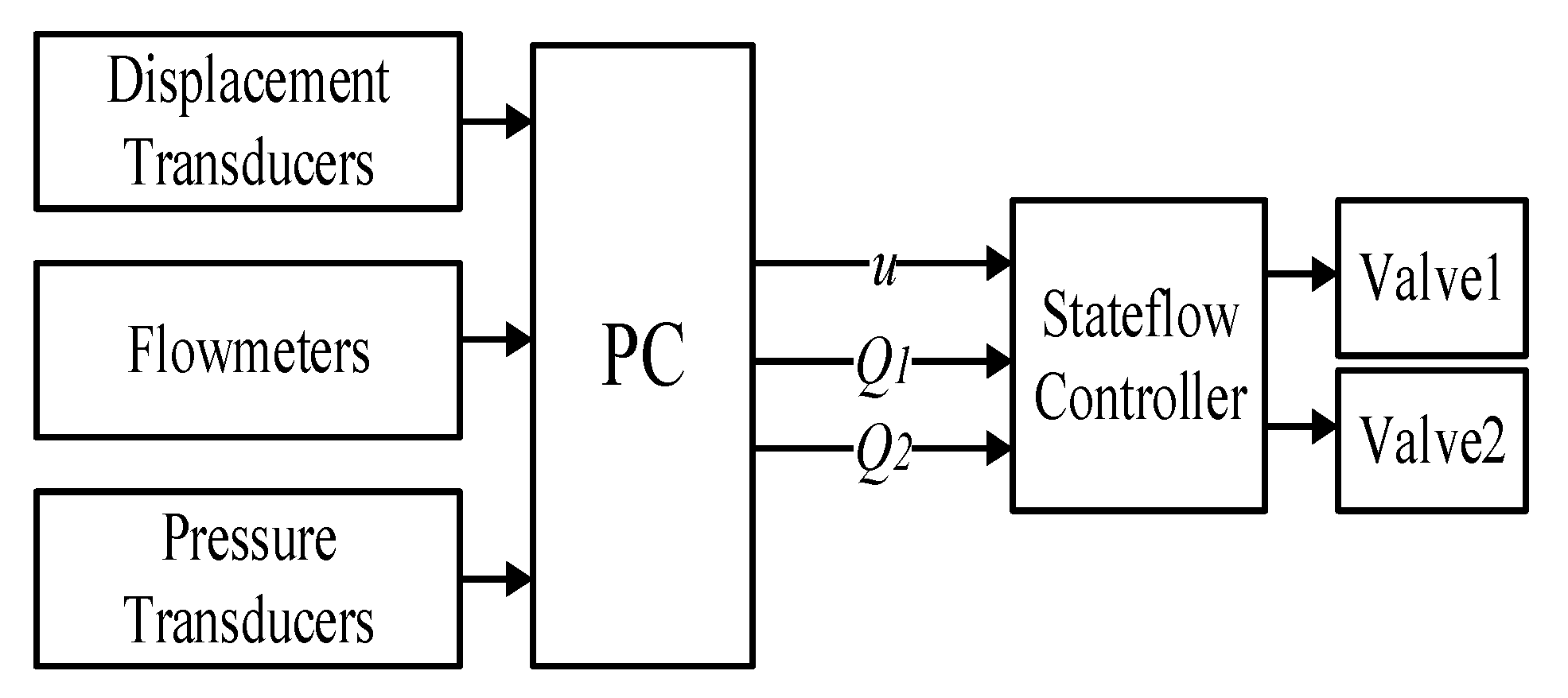
4. Stateflow Controller

Figure 9 shows the schematic of the electronic controller for a ZFS control system. Position of the cylinder piston, flowrate of hydraulic lines, and system pressures are collected by the transducers and sent to a PC. When it is ready to switch off the control line, the PC sends a command to a stateflow controller. At the same time, the flowrate of Q₁ and Q₂ are also sent to the stateflow controller.

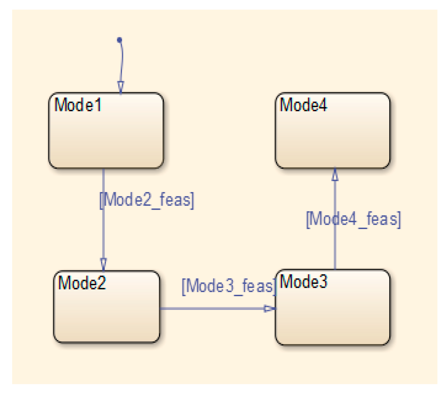
The stateflow chart (shown in Figure 10) determines the running mode of the system. When the stateflow controller receives command u from the PC, the system automatically runs in mode 1; when u = 1 is true, the controller is switched to mode 2; when Q₁ = 0 is true, the controller is switched from mode 2 to mode 3; when Q₂ = 0 is true, the controller is switched to mode 4. The conditions are defined as:

Mode 1_feas: u = 0,

(28)

Mode 2_feas: u = 1,

(29)

Mode 3_feas: Q₁ = 1,

(30)

Mode 4_feas: Q₂ = 1,

(31)

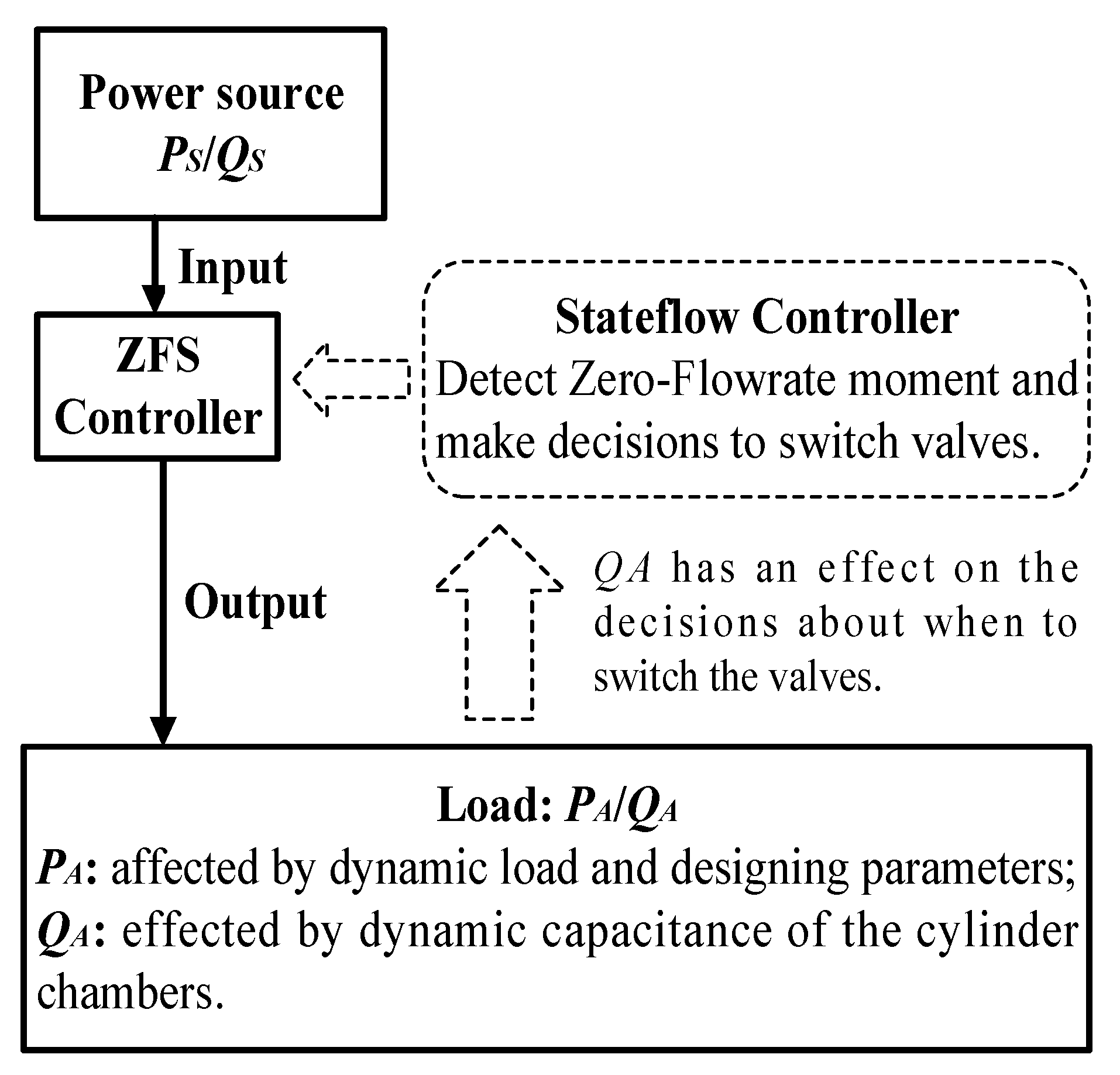
Figure 11 shows the relationship between the performance of a ZFS controller and some parameters of the system. The power source provides PS/QS as an input of the ZFS controller. Most piston pumps are feasible options to pressurize the system with proper pressure waves due to the reciprocating movement of the pistons. The output of the ZFS controller is defined by system parameters: the PA is required by the velocity and dimensions of the cylinder, as well as the exerted load force on the cylinder rod. The QA basically adapts the velocity of the cylinder. The capacitance of the cylinder would also have an effect on the QA, since a large derivation of the load force creates a certain flowrate within a fixed volume (the cylinder chamber can be regarded as a fixed volume when the time derivation is very small). A stateflow controller is employed to detect zero-flowrate moments and make decisions about when to switch the valves.

In this section, the output P_A and Q_A are modeled taking into consideration the dynamic load of the system and the dynamic capacitance of the cylinders. The models of switching power loss are built for both valves in the ZFS controller based on a linear characteristic of the valve opening. The pressure pulses are modeled for both valves in a ZFS controller according to the principle of fluid energy. All the models are built based on the following assumptions:

(1)

The pump outputs sinusoidal pressures at one frequency.

(2)

All the valves switch at zero-flowrate moments.

(3)

The opening of the valves changes linearly during switching processes.

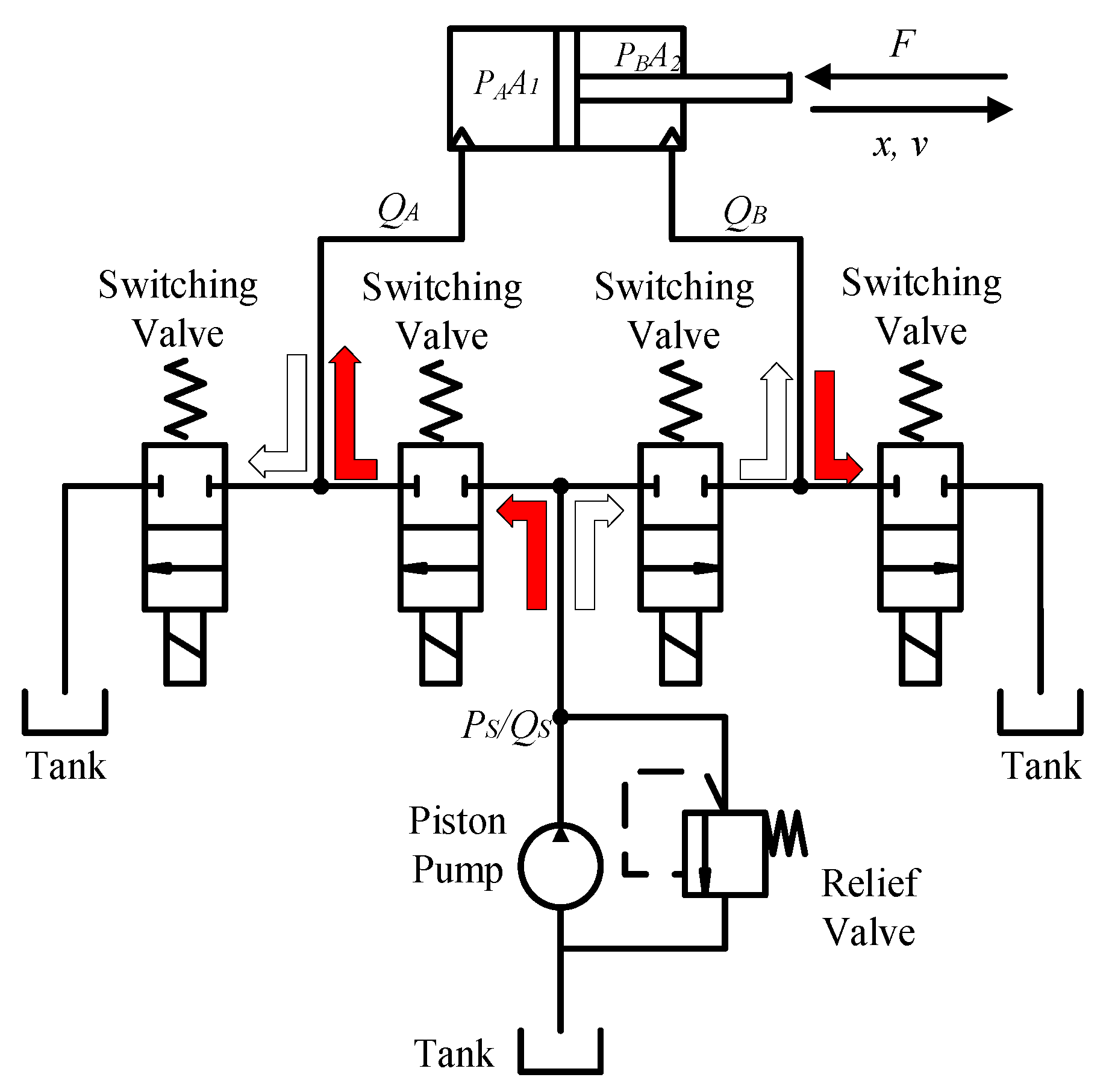
5. System Evaluation

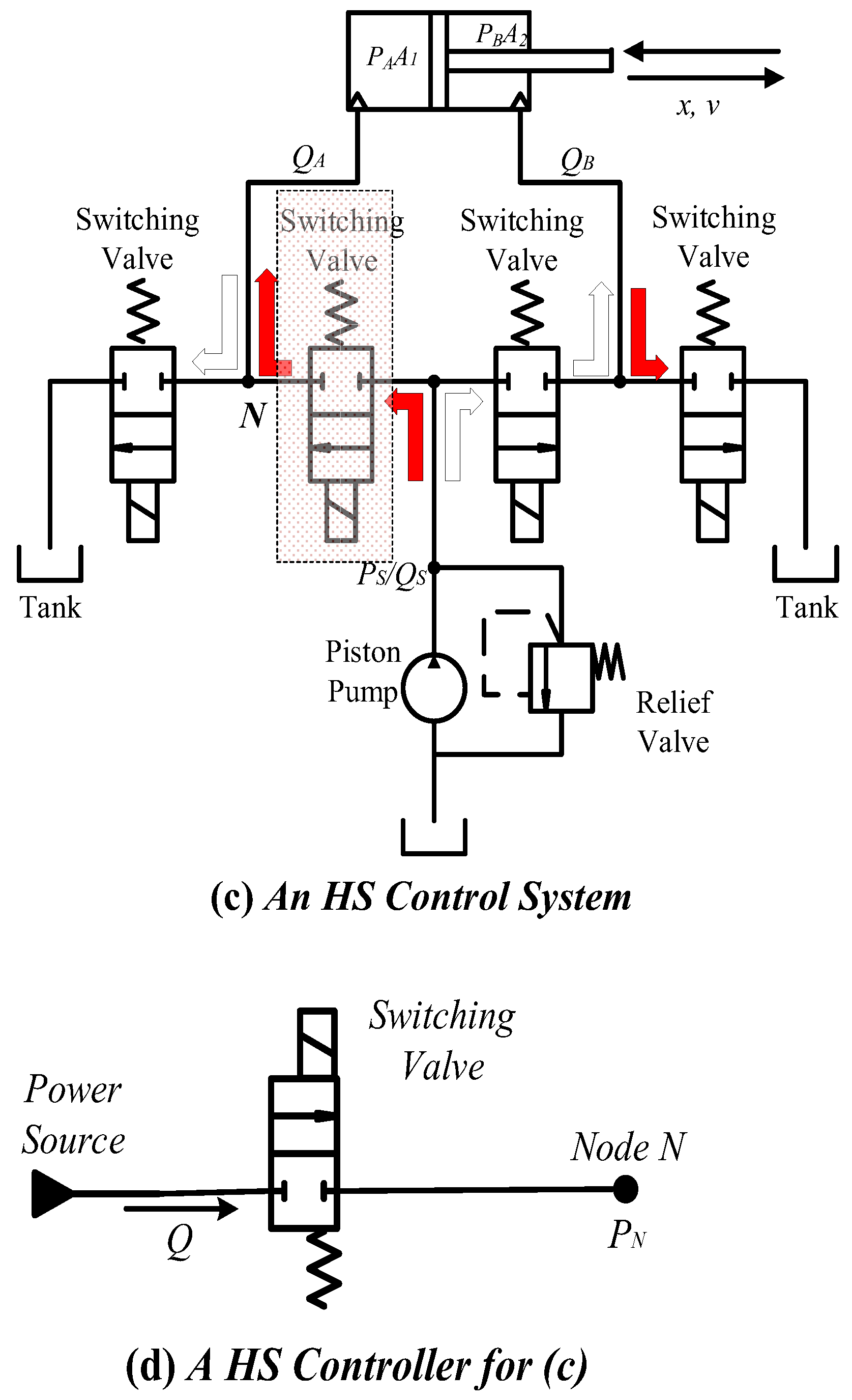
A dynamic ZFS controller (shown in Figure 12a,b) and a Hard-Switching (HS) system (shown in Figure 12c,d) are built for evaluation. A hydraulic inductance is realized by a piece of pipe with a length of 0.2 m and diameter of 0.008 m. A hydraulic capacitance is realized by an accumulator with a linear spring; the volume of the accumulator is 0.8 L.

The characteristics of the two systems are evaluated in this section. The dynamic capacitance, switching power loss and pressure pulses due to the switching-off of the valves are analyzed, respectively.

The tested systems are operated to drive a load at the speed of 0.06 m/s and with a load force of 40,000 N. The system pressure is 205 bar with waves whose amplitude and frequency are 2 bar and 113 Hz, respectively. The maximum flowrate of the pump is 7.5 L/min. Other parameters of the systems are presented in

Table 2. System parameters.

Parameters	Values
$\rho$	860 kg/m3
E	14,000 bar
V	0.8 L
D	0.008 m
l	0.2 m
f	113 Hz
$P_{Sa}$	2 bar
$P_{S0}$	205 bar
PA	203.8 bar
Qnorm	20 L/min@5 bar
v	0.06 m/s
QSmax	7.5 L/min

.

5.1. Dynamic Capacitance of the Cylinder

When the piston of the cylinder is moving, the volume of the cylinder chamber is varied; the varied chamber shows capacitance when the load force is changing. Such dynamic capacitance leads to flowrate change. According to Equation (12), the pipe volume and piston area have an effect on the flowrate change. Figure 13 presents a linear relationship between the position of piston x and the derivation of flowrate dQ. The piston area is 0.002 m², the diameter of the pipe of 0.012 m and the length of the pipe is 1 m. As the position of piston x increases from 0 m to 0.2 m, the derivation of flowrate dQ linearly increases correspondingly. When dF is 200 N, the derivation of flowrate dQ is relatively small and the slope of the curve is small; as dF increases, both dQ and the slope of the curve respond to this increase.

Figure 14 presents the relationship between the piston area and the flowrate change when the position of piston x = 0.2 m. When dF is fixed, it shows that the smaller the area of the piston is, the larger the derivation of the flowrate is. When the flowrate change dQ becomes infinitely large, then the area of the piston A_pis becomes infinitely small.

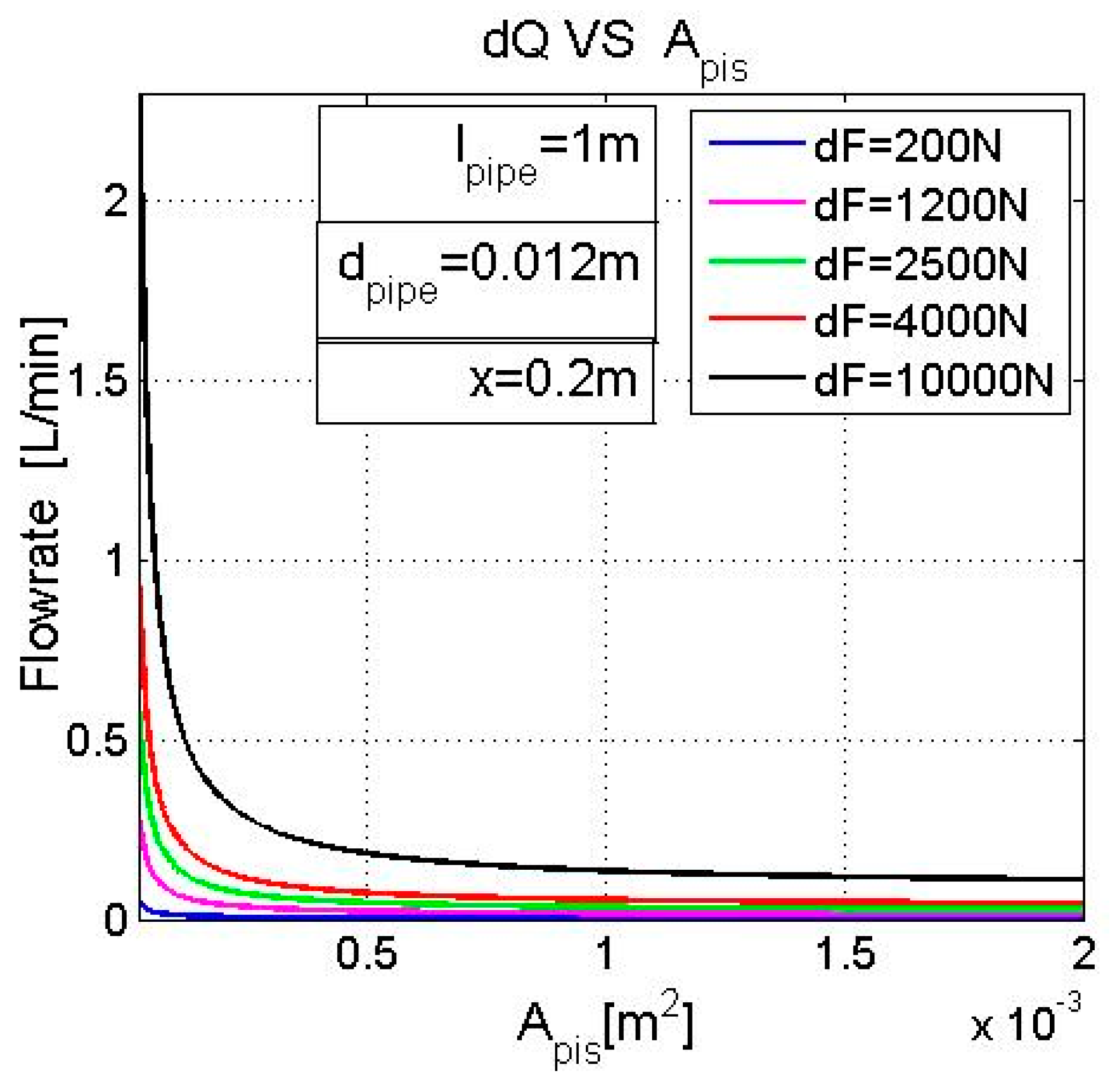
When the area of the piston is A_pis fixed, the derivation of flowrate dQ changes as the derivation of force dF increases. Take A_pis = 5 m², for example; the derivations of the flowrates are dQ = 0.0038 L/min when dF = 200 N, 0.023 L/min for when dF = 1200 N, 0.053 L/min when dF = 2500 N, 0.073 L/min when dF = 4000 N and 0.2 L/min when dF = 10,000 N.

A similar effect, the one the area of piston A_pis has on the derivation of flowrate dQ, is found in Figure 15. For a fixed pipe length l_pipe, the smaller the area of piston A_pis is, the larger the derivation of flowrate dQ is. Figure 14 also presents the relationship between the piston area A_pis and the flowrate change dQ. When dF changes from 200 N to 10,000 N, generally speaking, dQ increases as the length of the pipe l_pipe increases. When l_pipe is 0 m, the line is flat and straight; when l_pipe is larger, A_pis has more of an effect on dQ in small, scaled devices. By comparing the five figures with each other, a larger dF leads to a larger dQ. When dF is 10,000 N and A_pis is 0.002 m², dQ is 0.1 L/min.

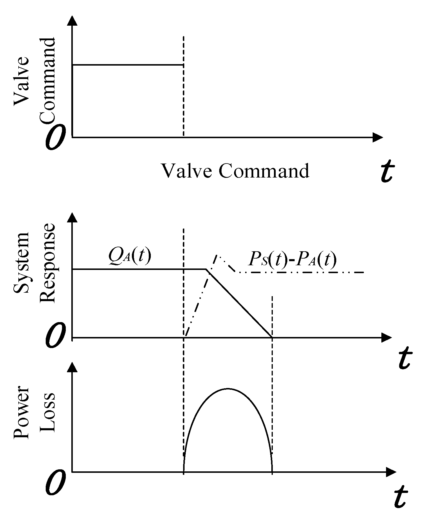
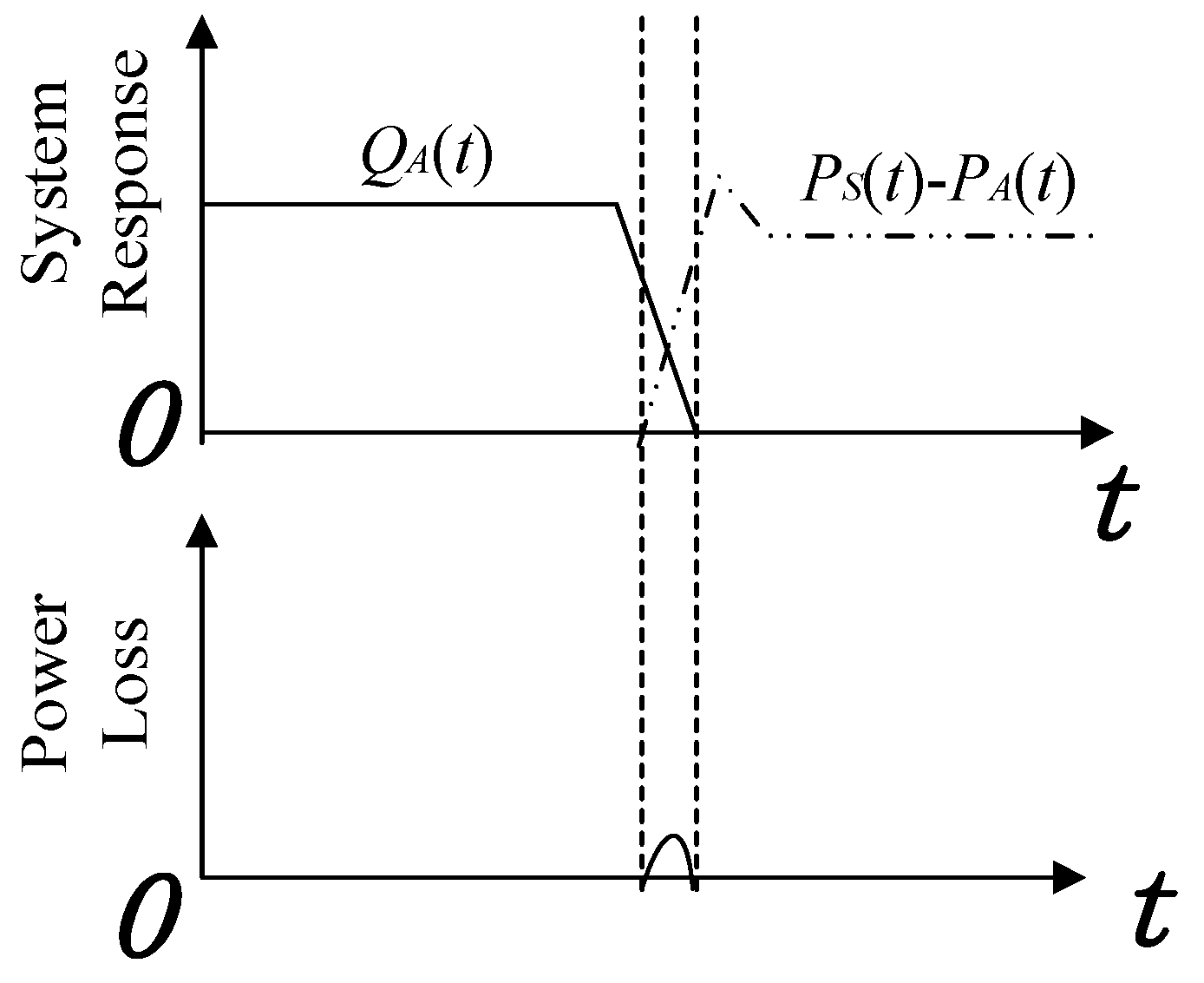
5.2. Switching Power Loss

The switching power loss is also investigated for the two models. Figure 16 and Figure 17 show the system responses for the dynamic ZFS system and HS system. In Figure 16, valve 2 is switched on at the end of mode 2. Then, the flowrate of the accessory line Q₁ decreases as the flowrate of the main line Q₂ increases. Q₁ falls down to zero and then valve 1 stays closed. Q₂ keeps going up and then falls down until its value is less than the load flowrate Q_A. Then, the supply flowrate supplies the system together with the resonant flowrate. The resonant flowrate falls down to zero and then goes in the opposite direction. Once the value of the resonant flowrate achieves the maximum supply flowrate Q_Smax, the flowrate Q₂ starts to decrease from Q_A until it reaches zero. Then, valve 2 is switched off. 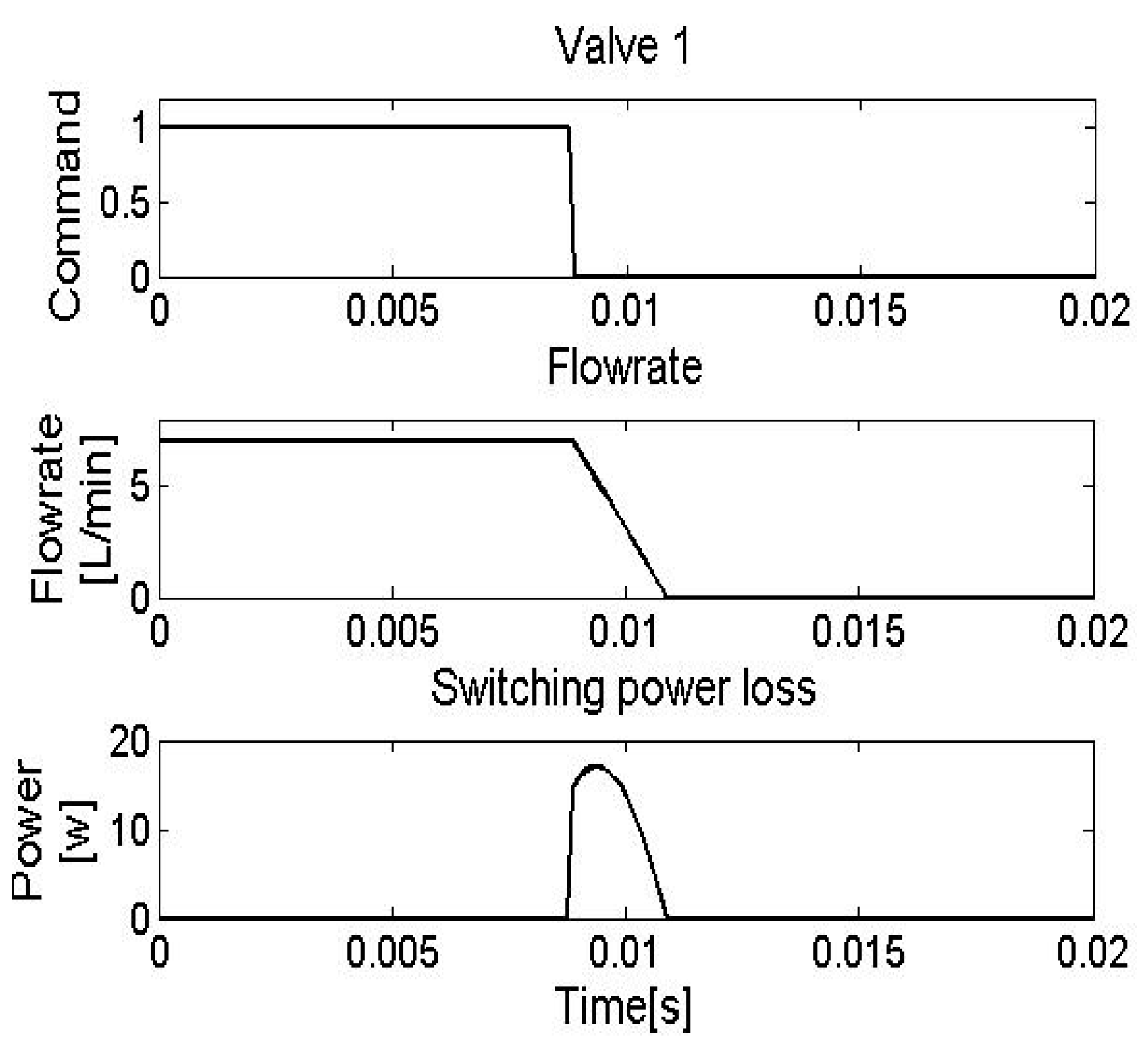Q₂ finally stays at zero after valve 2 is completely switched off.

According to the fifth plot in Figure 16, switching power loss occurs during two stages: one is for valve 1 and the other is for valve 2. The peak power losses are 4 w and 0.4 w for the two stages, respectively, compared to 17 w for the HS system (shown in Figure 17).

Table 3. Switching power loss for two systems.

	FS	HS
Valve 1	8.3 J	203 J
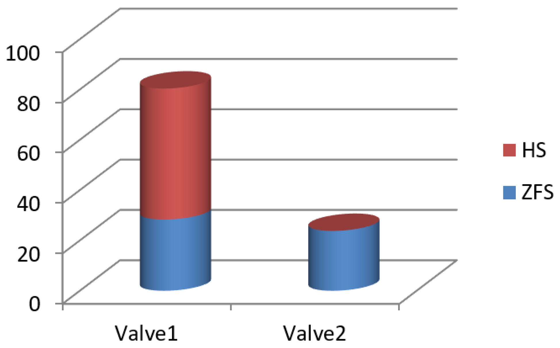
Valve 2	3.61 J	0 J

presents the energy consumptions of the two systems. The total switching power loss consumed by the ZFS system is 32 J versus 203 J consumed by the HS system (shown in Figure 18 and Table 3).

5.3. Pressure Pulses

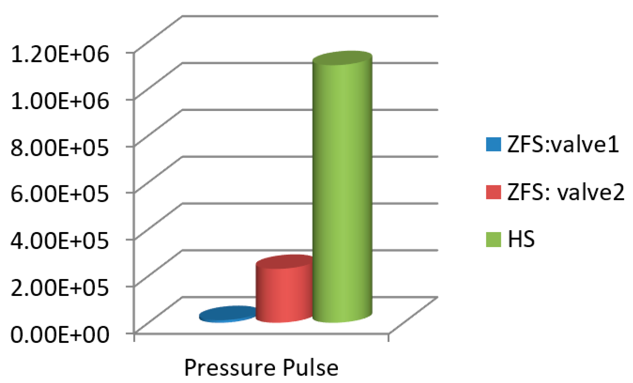
As shown in Figure 19 and

Table 4. Pressure pulses for two systems.

	ZFS: Valve 1	ZFS: Valve 2	HS
Pressure Pulse	1.1 × 104 Pa	2.3 × 105 Pa	1.1 × 106 Pa

, one switch in a normal HS controller excites pressure pulses with a peak value of 1.1 × 10⁶ Pa, while the peaks of the pressure pulse are 1.1 × 10⁴ Pa and 2.3 × 10⁵ Pa for valve 1 and valve 2, respectively. Pressure pulses in a ZFS system are much minor than those in a HS system.

6. Conclusions

In hydraulic applications, the switching-off of fast-switching valves leads to considerable switching power loss and pressure pulses. In this work, a dynamic ZFS controller is proposed to switch off valves at zero-flowrate moments. With the novel controller, the system achieves small switching power loss and suffers minor pressure pulses.

To better simulate zero-flowrate moments and make the switching power loss as small as possible, this paper takes into account the models of dynamic load forces and cylinder capacitance. In the following applications, dynamic load forces and cylinder capacitance should be considered when running a ZFS controller:

(1)

Applications where the cylinder stroke is large.

(2)

Applications where the derivation of load forces is large.

(3)

Applications where the piston/rod areas of the cylinders are small.

(4)

Applications where the pipe length between the output of the ZFS controller and the input of the cylinder is large.

The results show the advantage of a dynamic ZFS system in relation to its energy saving performance. The total switching power loss consumed by the ZFS system is 32 J versus 203 J consumed by the HS system. The system applying the dynamic ZFS controller consumes only 16% of the energy that is consumed by a normal HS system.

Moreover, the system with a dynamic ZFS controller leads to minor pressure pulses. One switch in a normal HS controller excites pressure pulses with a peak value of 1.1 × 10⁶ Pa, while the peaks of the pressure pulse are 1.1 × 10⁴ Pa and 2.3 × 10⁵ Pa for valve 1 and valve 2, respectively. Pressure pulses in a dynamic ZFS system are much minor than those in a HS system.

It can be concluded that the dynamic ZFS controller provides a solution to achieve better efficiency performance and make pressure pulses as minor as possible in typical four-ports hydraulic systems. Besides in typical 4-ports hydraulic systems, switching also exists in traditional proportional/servo hydraulic systems where high frequency-switching happens. The ZFS control method provides a potential solution for those systems with large switching power loss and unsmooth pressure response caused by valve switching.