Article

An Obstacle-Avoidance Motion Planning Method for Redundant Space Robot via Reinforcement Learning

1
School of Automation, Beijing University of Posts and Telecommunications, Beijing 100876, China
2
Beijing Aerospace Control Center, Beijing 100094, China
3
Technology and Engineering Center for Space Utilization, Chinese Academy of Sciences, Beijing 100094, China
*
Author to whom correspondence should be addressed.
Actuators 2023, 12(2), 69; https://doi.org/10.3390/act12020069
Submission received: 18 January 2023 / Revised: 5 February 2023 / Accepted: 6 February 2023 / Published: 8 February 2023
(This article belongs to the Special Issue Advanced Spacecraft Structural Dynamics and Actuation Control)

Abstract

:
On-orbit operation tasks require the space robot to work in an unstructured dynamic environment, where the end-effector’s trajectory and obstacle avoidance need to be guaranteed simultaneously. To ensure the completability and safety of the tasks, this paper proposes a new obstacle-avoidance motion planning method for redundant space robots via reinforcement learning (RL). First, the motion planning framework, which combines RL with the null-space motion for redundant space robots, is proposed according to the decomposition of joint motion. Second, the RL model for null-space obstacle avoidance is constructed, where the RL agent’s state and reward function are defined independent of the specific information of obstacles so that it can adapt to dynamic environmental changes. Finally, a curriculum learning-based training strategy for RL agents is designed to improve sample efficiency, training stability, and obstacle-avoidance performance. The simulation shows that the proposed method realizes reactive obstacle avoidance while maintaining the end-effector’s predetermined trajectory, as well as the adaptability to unstructured dynamic environments and robustness to the space robot’s dynamic parameters.

1. Introduction

With the development of aerospace technology, space exploration activities become increasingly frequent, and the on-orbit operations, such as spacecraft assembly, maintenance, debris removal, etc., become urgent demands. The space environment has the features of no gravity, no air and high radiation, which makes astronauts face great safety risks when performing on-orbit operations. As a type of typical aerospace equipment, space robots have high autonomy and flexibility, so they are widely used in various on-orbit tasks instead of astronauts [1,2]. Moving or carrying loads safely to the target position is the basic operation in on-orbit operations and also should be the most basic function for space robots. In general, a space robot is composed of a base with control system and solar arrays, as well as a manipulator with several links and an end-effector which carries the load. Therefore, safely moving contains two meanings: Firstly, a smooth, collision-free trajectory for the load should be provided so that it can reach the target position along this trajectory. Secondly, the body of the space robot, especially the links of the manipulator, needs to avoid obstacles in the environment as the load moves along this trajectory. These two conditions should be met simultaneously, which derives the obstacle-avoidance motion planning for the space robot [3].
Obstacle-avoidance motion planning is a long-term direction in robotic research. Some methods, such as visibility graph [4], Voronoi diagram [5], probabilistic roadmap method (PRM) [6], rapidly exploring random tree (RRT) [7], A* algorithm [8], etc., are widely used in robotic community. Most of the above methods are aimed at stationary obstacles or the situations, where environmental information is known. However, the working environment of space robot is unstructured and dynamic. There are not only stationary obstacles, but also moving obstacles that cannot be predicted to their moving trajectories (e.g., floating debris, and unfixed tools), requiring the obstacle-avoidance motion planning method to be real-time. Similar to the biological stimulus–feedback mechanism, Khatib [9] proposed a reactive obstacle-avoidance method based on artificial potential field (APF), which enables real-time response to unstructured dynamic scenes. However, it only constrains the end-effector’s target position while not the whole trajectory. As a result, the end-effector’s predetermined trajectory for the task cannot be guaranteed if the obstacle approaches, which means this method cannot be applied to the tasks that have requirements on the end-effector’s trajectory. For this problem, researchers noticed that the redundant degrees of freedom (DOF) of the manipulator can be used to track the end-effector’s predetermined trajectory while avoiding obstacles. It uses the null-space motion characteristic of the redundant robot. According to this, many solutions have been proposed, such as null-space vector assignment [10], redundant manipulator-based APF [11,12], gradient projection method (GPM) [13,14], objective function optimization [15,16], etc. Among them, redundant manipulator-based APF and GPM are the common used methods with high efficiency in practice.
In fact, for on-orbit operation tasks, there are strict requirements for the end-effector’s trajectory, such as maintenance, grasping, and docking, etc., which requires the space robots to avoid unpredicted moving obstacles as much as possible on the premise of ensuring the tracking of the end-effector’s predetermined trajectory. Even partial contact or slight collision is allowed in extreme cases, such as emergency repair on critical fault. Fortunately, most space robots have redundant DOFs, it means that we can tap the potential of obstacle avoidance as much as possible without changing the end-effector’s trajectory. However, unlike the ground robot, there is a motion coupling between the free-floating base and the manipulator of the space robot. Once the manipulator’s joints are actuated, the end-effector and the base will move at the same time so that the identical method to the ground robot cannot achieve the desired effect of obstacle avoidance. At present, the most active research in this field is GPM and the objective function optimization method. Mu et al. [17] constructed a unified framework to model the obstacles for a redundant space robot, and combined GPM to obtain the collision-free trajectories. Hu et al. [18] proposed the gradient projection weighted Jacobian matrix (GPWJM) method, which takes the end-effector’s trajectory tracking as the main task, as well as meeting the motion constraints of the base and links. Wang et al. [19] described the target position arrival and obstacle avoidance as linear inequality constraints, then integrated them into a quadratic programming (QP) optimization to calculate the trajectory with the help of non-linear model predictive control (NMPC). Ni et al. [20] transformed the motion planning problem into a multi-objective optimization that achieves the target configuration while avoiding obstacles, which is solved by the particle swarm optimization (PSO) method. Rybus et al. [21] introduced joint splines into motion planning, then constructed a constrained nonlinear optimization problem to solve the collision-free and task-required trajectory, which used the active set method to generate the solution. However, the above methods introduce complex solution strategies and operation rules, including differentiation, integration and nonlinear functions, which reduces the computational efficiency. For the space robots with limited computing resources, low computing efficiency will seriously affect the task performance.
Recently, with the development of reinforcement learning (RL) theory, new solutions have been provided to solve the problem of reactive obstacle-avoidance motion planning for unpredicted moving obstacles. RL builds an agent that continuously interacts with the environment, which optimizes its own action generation policy according to the feedback states and rewards from the environment during each interaction process so as to maximize the sum of rewards. It has good environmental adaptability and computational real-time performance, such as DDPG [22,23], TD3 [24], PPO [25], SAC [26], etc., showing great potential in robotics applications. These methods can generate safe and collision-free trajectories from the specified start point to target point based on the feedback states from the unstructured dynamic environment, but most of them are aimed at mobile robots that can be regarded as moving particles. For the robots with a chained manipulator, such as service robots and industrial robots, the research focus is on the completion of manipulation tasks, which means that the designed RL structures lack native obstacle-avoidance mechanisms. Their state space and rewards lack the representation of obstacle information [27], or only aim at some specific obstacles [28] such that these methods are difficult to be applied to unstructured dynamic environments, where the number and motion state of the obstacles are not specified. When there are unexpected obstacles which do not exist during the training process, they are difficult to achieve effective obstacle avoidance, unless a large number of randomly moving obstacles are introduced during training, or retraining a new policy for the changed environment. However, adopting these methods will also greatly reduce the training efficiency of RL. In terms of space applications, the research on RL-based spacecraft control to improve its autonomous decision-making performance has made a lot of progress, including spacecraft landing on celestial bodies, maneuver planning, attitude controlling, rover path planning, etc. [29]. Most of these methods also regard the spacecraft as a mobile robot with special motion response in space, rather than a ground industrial or service robot with a chain manipulator, so they cannot achieve on-orbit operation tasks. However, unlike the ground chain manipulator, using RL to achieve obstacle avoidance is more difficult for space robots due to the free-floating characteristic of the base. Yan et al. [30], Du et al. [31], and Wu et al. [32] explored the application of RL in space robots, preliminarily proving that RL methods, such as soft Q-learning and DDPG can achieve effective motion planning and control for the space robot with free-floating base, but obstacle avoidance was not discussed. Wang et al. [33] developed a model-free hierarchical decoupling optimization (HDO) algorithm for space robots. The upper layer uses RRT to sample collision-free path points, while the lower layer uses DDPG to connect each sampling point, so the collision-free motion trajectories can be generated. Li et al. [34] combined DDPG and APF, then introduced the self-collision avoidance constraints of the end-effector to realize the motion planning. Although these methods can be applied to redundant space robots, they do not have the ability to maintain the end-effector’s predetermined trajectory during the obstacle-avoidance process. As mentioned above, this ability is very important for the space robot.
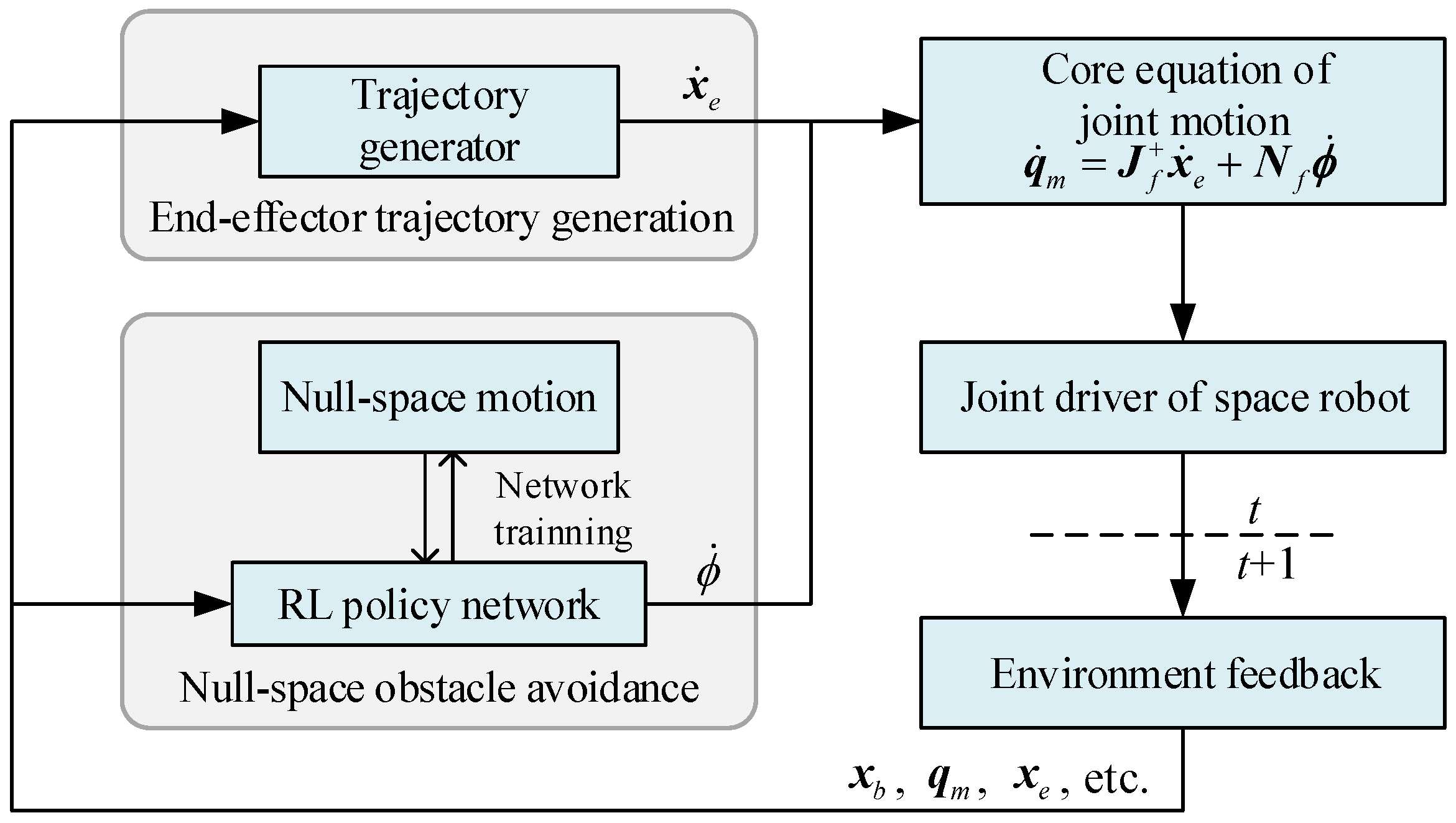
In summary, considering the on-orbit operation constraint of obstacle-avoidance motion and inspired by GPM, we propose a new obstacle-avoidance motion planning method for redundant space robots by combining the null-space motion with reinforcement learning. Unlike PRM, RRT and other obstacle-avoidance methods which cannot constrain the end-effector’s movement, our method can realize reactive obstacle avoidance while maintaining the end-effector’s predetermined trajectory with good adaptability to the unstructured dynamic environment, which can cope with the changes of obstacles in the environment without retraining. The major contributions of this paper are as follows:
  • The motion planning framework combining RL with null-space motion for space robots is proposed to realize reactive obstacle avoidance without changing the end-effector’s predetermined trajectory.
  • The RL agent’s state space and reward function independent of the specific information of obstacles are defined from the aspect of the robot itself, so that the RL agents can be applied to unstructured dynamic environments, avoiding retraining for obstacle changes.
  • A curriculum learning-based training strategy for RL agent is designed to further improve the sample efficiency, training stability and performance of the obstacle avoidance.
The rest of this paper is organized as follows: In Section 2, the proposed motion planning framework is introduced, which contains the end-effector trajectory generation module and the RL-based null-space obstacle-avoidance module. In Section 3, the RL paradigm for null-space obstacle avoidance module, as well as state space, action space, reward function, and the curriculum learning-based training strategy, are described in detail. In Section 4, the simulation results are presented and discussed. Finally, the conclusions of this paper are given in Section 5.

2. Motion Planning Framework

In this section, the motion trajectory of robot joints is decoupled into task-required motion components and task-independent null-space motion components according to the redundancy and free-floating characteristic of the space robot. Then the RL-based obstacle-avoidance motion planning framework is proposed to meet the requirements of task execution, together with obstacle avoidance in an unstructured environment.

2.1. Joint Motion Decomposition

As Figure 1 shows, assume that the space robot is composed of a base with s motion dimensions and a manipulator with n joints, where s = 3 if the space robot always moves on a plane (i.e., planar space robot), while s = 6 if the space robot moves in three-dimensional space. The motion of the end-effector is the superposition of the base motion and the joint motion [35], which can be expressed as
x ˙ e = J b x ˙ b + J m q ˙ m
where x ˙ e is the velocity vector of the end-effector, x ˙ b is the velocity vector of the base, q ˙ m is the angular velocity vector of the joints; J b is the Jacobian matrix describing the mapping relationship between the base velocity and end-effector velocity, which is related to the pose of the base x b ; and J m is the Jacobian matrix describing the mapping relationship between the angular velocity of each joint and the end-effector velocity, which is related to the configuration of the manipulator q m .
Because of the free-floating characteristic on orbit, there is a coupling relationship between the joint motion and the base motion as
x ˙ b = J b m q ˙ m
where J b m is the mapping matrix from joint angular velocity to base velocity, which is related to x b and q m . Substituting Equation (2) into Equation (1), we can obtain
x ˙ e = J b J b m + J m q ˙ m = J f q ˙ m
According to Equation (3), we know that if the pose of the base and the configuration of the manipulator are specified, the end-effector velocity is only determined by the joint angular velocity.
If n > s , i.e., the number of joints of the manipulator is greater than the motion dimension, the space robot has n s redundant DOFs. In this situation, there can be multiple sets of manipulator configurations that meet the specified pose of the end-effector. For Equation (3), this characteristic can be expressed as
q ˙ m = J f + x ˙ e + N f ϕ ˙ = J f + x ˙ e + I J f + J f ϕ ˙
where J f + is the Moore–Penrose pseudoinverse of the space robot Jacobian J f ; N f = I J f + J f is the null-space mapping matrix; ϕ ˙ R n × 1 is the joint null-space velocity vector so that N f ϕ ˙ constitutes the null-space term of the solution of equation x ˙ e = J f q ˙ m , which means that for ϕ ˙ R n × 1 , q ˙ m = N f ϕ ˙ makes the equation J f q ˙ m = 0 always hold.
Therefore, for a free-floating space robot with redundant joints, the joint motion can be decomposed into two components: one component tracks the motion of the end-effector, and the other moves the base and links while keeping the pose of end-effector unchanged (called null-space motion component). Planning the trajectory of term x ˙ e can make the end-effector of the space robot move along the task-required path. Simultaneously, the obstacle avoidance of the links can be realized by choosing different ϕ ˙ in the unstructured dynamic environment.

2.2. Design of the Motion Planning Framework

The space robot needs to reach the target position along the predetermined trajectory in the unstructured dynamic environment. During this process, if the distance between the space robot and the obstacle is less than the specified safe distance, the space robot should perform the action for obstacle avoidance, as shown in Figure 1. Therefore, according to the motion decomposition in the previous section, we propose an RL-based obstacle-avoidance motion planning framework for a redundant space robot, as shown in Figure 2.
It can be seen from the above figure that the proposed motion planning framework includes two main modules: the end-effector trajectory generation module and the null-space obstacle-avoidance module. The former generates the end-effector velocity x ˙ e according to the current feedback information, such as the pose of the base and end-effector, the configuration of the manipulator, etc. The latter generates the null-space solution vector ϕ ˙ according to the joint angle, the distance of environment obstacles and the other information. The outputs of these two modules are superimposed by the core equation of joint motion Equation (4) to form the final joint angular velocity of the manipulator q ˙ m at current timestep t, which is used as the command of the joint controller to drive the space robot to track the desired end-effector trajectory. Then, through the environment feedback again, the state information required by the two modules at the next timestep is obtained, and the corresponding control command for the next timestep is then generated.
Since Equation (4) completely decouples the joint angular velocity with respect to the end-effector velocity component and the null-space velocity component, the training and execution of these two modules can be carried out independently, which provides great convenience for the design and improvement of motion planning strategies.

3. Null-Space Obstacle Avoidance Based on RL

Reinforcement learning has excellent environmental adaptability. After training is accomplished, RL can generate instant actions for environmental changes, which is suitable for the applications in dynamic scene. Considering the dynamic and unstructured characteristics of the working environment of space robots, we design the details about the RL-based null-space obstacle-avoidance strategy, which prevents the collision between the links and the obstacles, simultaneously maintaining the current pose of the end-effector.

3.1. RL Model for Null-Space Obstacle Avoidance

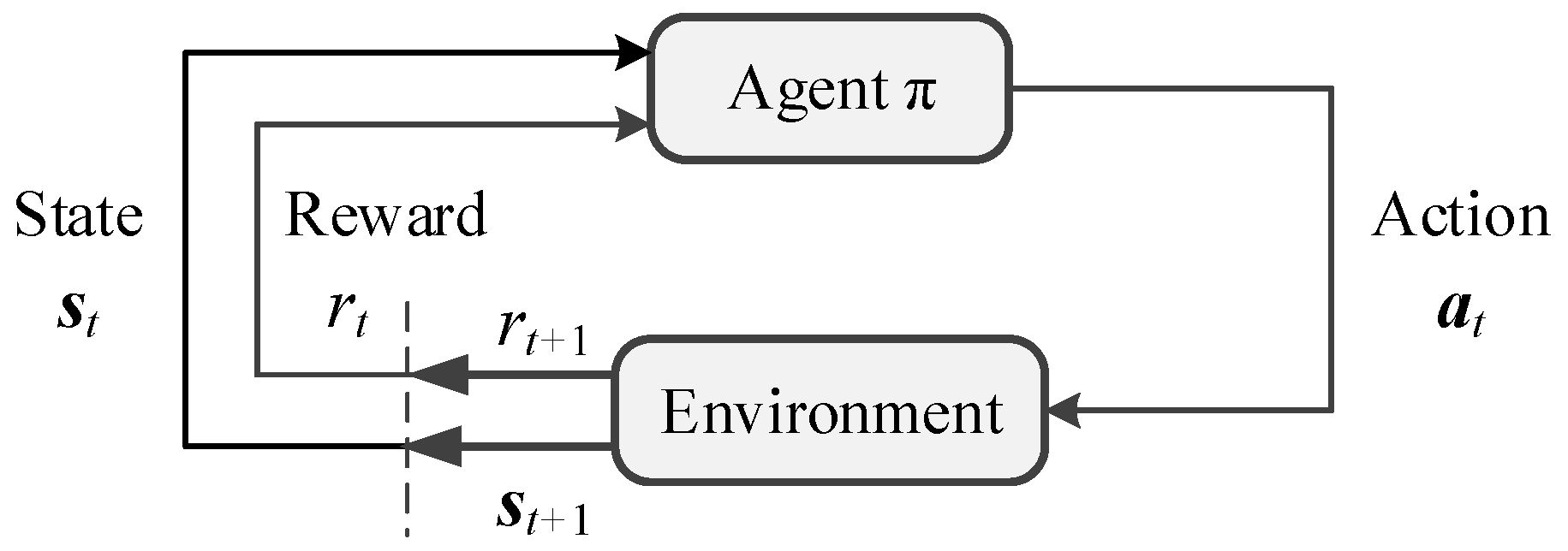
In order to introduce RL to realize null-space obstacle avoidance, we should transform this task into a mathematical paradigm for RL problems. The main idea of RL is that the agent continuously interacts with the environment to adjust and optimize its action policy according to the feedback states and rewards from the environment during each interaction so as to maximize the sum of rewards after the task is completed. The process of RL is shown in Figure 3.
As shown in Figure 3, the agent is constantly maintaining an action generation policy π . For each timestep t, the agent obtains the current state vector s t S and the feedback reward r t R from the environment, where S represents the state space composed of all possible states in the environment, and R is the set of real numbers. If the policy π has been trained and deployed, it generates the action a t A according to s t , where A represents the action space composed of all executable actions of the agent. Otherwise, the agent will make decisions based on its interaction experience, knowledge base or other manual methods to generate action a t . Subsequently, the action a t acts on the environment to obtain the state s t + 1 and reward r t + 1 at the next timestep. The above process is repeated over time. In this process, the agent will train or optimize its own action generation policy π according to the obtained reward. The ultimate goal of the agent is to train an optimal policy π to maximize the cumulative reward R t . It can be expressed as
R t = r t + 1 + γ r t + 2 + γ 2 r t + 3 + . . . = k = 0 γ k r t + k + 1
π = arg max π E k = 0 γ k r t + k + 1
where γ 0 , 1 is the discount factor of the reward.
For the null-space obstacle-avoidance of space robots, the agent is a certain policy π that generates the null-space angular velocity of the joints. The goal of this policy is to generate the null-space solution vector ϕ ˙ at the current timestep according to the feedback information—the states of the space robot and the positions of the obstacles in the environment—so that the manipulator can avoid the obstacles in an optimal way under a certain evaluation criterion.
Therefore, the action of the agent a t is the null-space solution vector, namely,
a t = ϕ ˙ t
The state of the agent s t consists of the information about the space robot and obstacles. In previous works [28], it is usually defined similar to
s t = q m t , x e t , x o t
where t is the timestep, q m t is the joint angle of the manipulator, x e t is the pose of the end-effector, and x o t is the position of the obstacle. The reward from the interaction between the agent and the environment r t is a feedback function, which is denoted as
r t = r s t , a t
It determines whether the space robot collides with obstacles, and evaluates whether the current configuration is reasonable so as to guide the policy’s training process. The specific forms of s t and r t in our method are defined in Section 3.2.
Unlike the traditional tabular RL methods, the action vector a t and state vector s t we defined are high-dimensional continuous and differentiable variables so that the RL agent must support continuous action/state space, and has the ability to prevent from “dimensional disaster” (i.e., inefficient or invalid learning in high-dimensional state space). Soft actor–critic (SAC) is the current state-of-the-art RL method, which is robust to the learning of continuous high-dimensional variables, such as robotics. Thus, we adopt SAC to optimize policy π for better training performance. It should be pointed out that, except for the requirement of continuous action/state space, our method does not specify the RL network structure and parameter optimization strategy. In fact, as mentioned in the introduction, there are many applications of robot planning or controlling with DDPG, PPO and the other RL methods. Here, we choose SAC, as it has higher data efficiency to avoid long-time training [26,36]. That is to say, if a better RL method is developed in the future, we can also use it instead of SAC. The policy π is described as a neural network with input s t and output a t , which is expressed as
a t = π θ s t
where π θ represents the neural network that constitutes the policy π , and θ is the parameters of the neural network. The idea of SAC is to add an entropy function into Equation (6) to enhance the randomness of policy exploration so as to accelerate the policy convergence during the training process. Thus, Equation (6) becomes
π = arg max π θ E t γ t r ( s t , a t ) + α H π θ ( s t )
where H · is the entropy function, which generates a random distribution that affects the direction of policy exploration according to the action of the neural network π θ ; α is the temperature of the entropy, which adjusts the ratio of the cumulative reward to the entropy value.
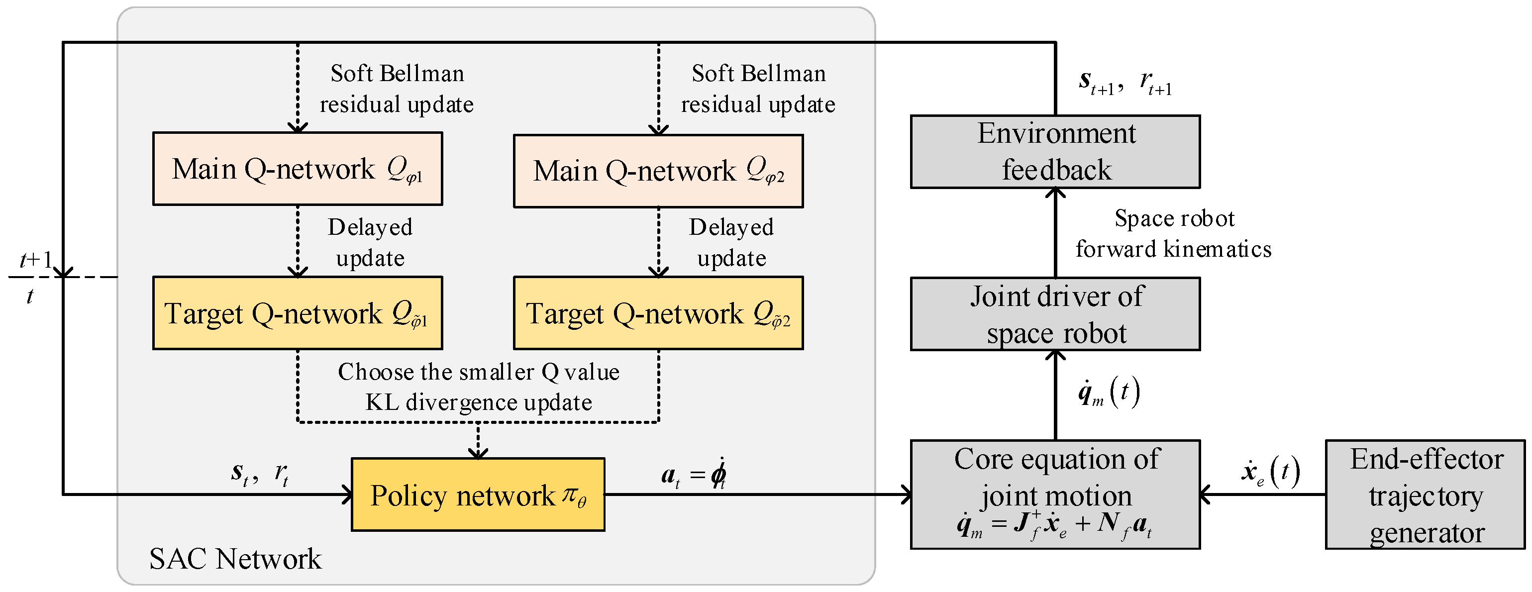
Specifically, SAC contains a policy network π θ that generates actual actions (i.e., the null-space solution vector ϕ ˙ for space robot), as well as two main Q-networks Q φ 1 , Q φ 2 and two target Q-networks Q φ ˜ 1 , Q φ ˜ 2 that evaluate the quality of the current policy, where θ , φ 1 , φ 2 , φ ˜ 1 , and φ ˜ 2 represent the parameter vectors of their corresponding networks, respectively. The network structure is shown in Figure 4. The detailed training process of SAC network is described in [26], and we do not explore it in this paper.

3.2. State and Reward Function Definition

It is important to choose appropriate states and reward function for solving the RL task of space robot obstacle avoidance. As mentioned above, in the previous RL-based robot planning methods, the state vector is mostly defined similar to Equation (8). However, this definition is only suitable for a fixed number of obstacles in the working environment. In the unstructured dynamic environment, the number of obstacles is usually unknown and even may change during task execution such that the defined state vector cannot match the actual working environment. It can only be solved by modifying the state definition and retraining for every change of the scene configuration, which is not practical to be deployed in reality.
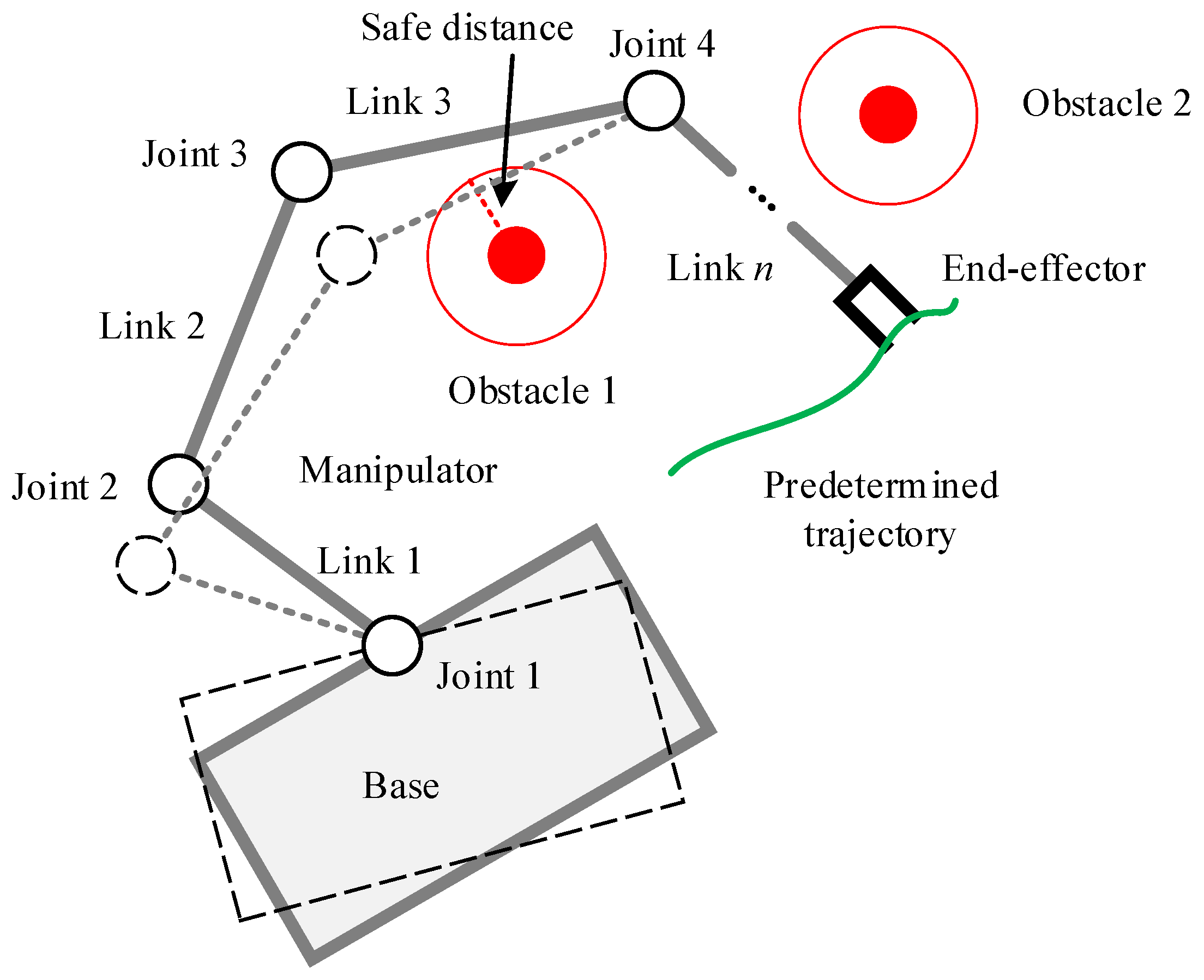
In our method, we treat the obstacles’ state from the perspective of the space robot itself to solve this problem, i.e., we use the vector p , which represents the distance of each link and its nearest obstacle to replace the obstacle position x o in Equation (8), as shown in Figure 5. Specifically, we number the space robot components with i = 0 n to represent the base as well as Link 1~Link n, respectively. Let P i r be the set that contains all the surface points’ position vectors of Component i, then let p i r P i r be a certain point’s position vector of Component i. Suppose there are k obstacles in the environment. Let P j o be the set that contains all the surface points’ position vectors of Obstacle j, where j = 1 k , then let p j o P j o be a certain point’s position vector of Obstacle j. Thus, the distance vector between each component of the space robot and the obstacle can be defined as
p i = arg min p i r P i r , p j o P j o , j = 1 k p j o p i r , i = 0 n
So p o represents the position vector of the two closest points between the base and the nearest obstacle, and p 1 ~ p n represent the position vector of the two closest points between Link 1~n and their nearest obstacle, respectively.
Therefore, the state vector of the RL model for null-space obstacle avoidance is defined as
s t = q m , q ˙ m , p 0 , p 1 , , p n
where q m and q ˙ m represent the configuration and joint angular velocity of the manipulator at timestep t; p 0 p n describes the influence of all the possible obstacles in the environment on the base and the links. It can be seen that the definition is independent of the environment-specific information, such as the number or the shape of obstacles, which ensures the generality of the strategy in various unstructured dynamic scenes. In addition, the action ϕ ˙ , which is generated by the policy network π θ , will not change the pose of the end-effector, so there is no need to add the related state variables (e.g., end-effector position x e , and velocity x ˙ e ) to the vector.
Then, we design the reward function of the environment feedback for the null-space motion of the space robot. Since the space robot needs to complete other operation tasks, such as expected trajectory tracking, it is necessary to make the null-space motion have higher stability and operability to prevent the space robot from generating an oscillating path or falling into the local optimum in the process of obstacle avoidance. For this purpose, we propose the following reward function:
r = λ 1 r o + λ 2 r a + f p i r c
In Equation (14), r o is the obstacle-avoidance feedback term, which is defined as
r o = i = 1 n min ln e b e a d s p i + e a b , 0
where d s is the specified safe distance between the space robot and the obstacle, and a and b are the scoping values. In particular, when the distance between the space robot components (the base or the links) and the single obstacle is less than d s , a negative log reward r o a b , 0 will be obtained, guiding the space robot to perform obstacle-avoidance operations. We set a = 1 and b = 0 empirically for normalization. r a is the motion stabilization term, which is defined as
r a = I J f + J f ϕ ˙
where I J f + J f ϕ ˙ is the angular velocity component of the joint null-space motion. A lower null-space angular velocity can prevent the manipulator from oscillating during the obstacle-avoidance process. λ 1 and λ 2 are the weights of r o and r a , respectively, which are used to adjust the relative size to keep the reward value r within a suitable range. r c is the collision penalty term with a large negative value, and f c p i is the indicator function that judges whether the collision has occurred, which is defined as
f c p i = 0 , if i = 0 n s . t . p i = 0 1 , else
Thus, once any component of the space robot collides with any obstacle, the RL agent will obtain a large negative reward value, then the current training episode will be terminated.

3.3. Training Strategy

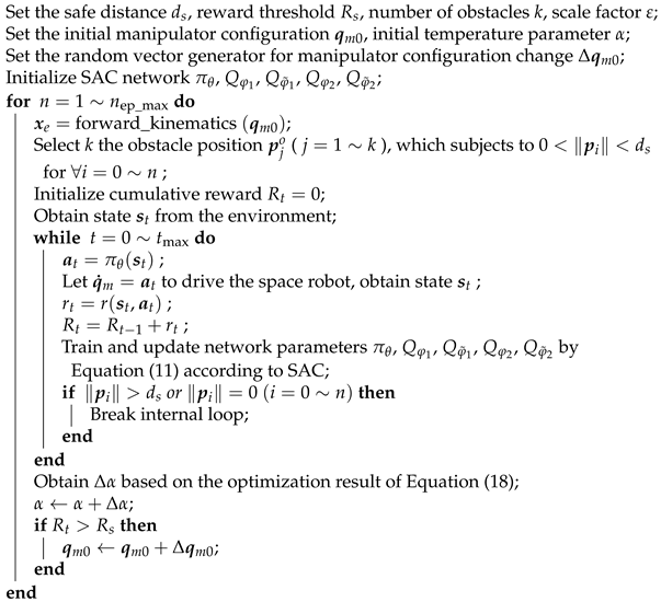
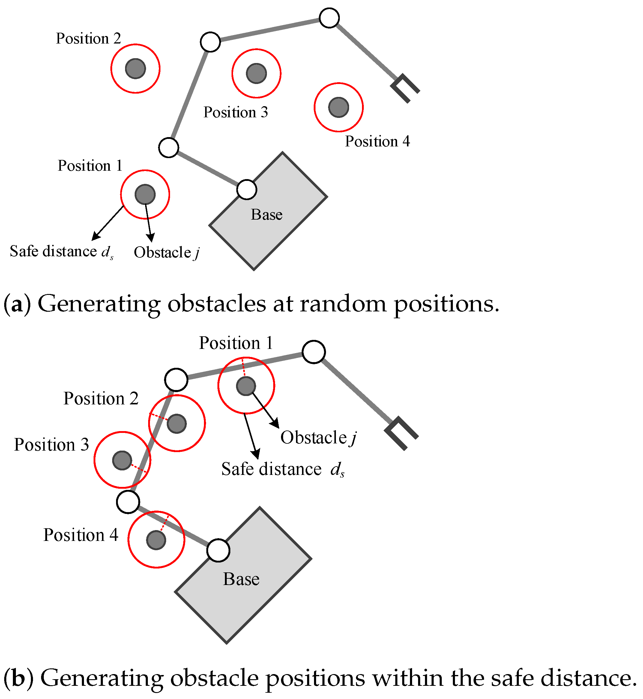
Usually, during the training of RL agent, the training environment is required to be as random as possible so as to ensure that the policy has sufficient generalization to deal with various environmental states. However, the obstacles only occupy a small part of the area compared to the workspace of the space robot so that in most randomly generated scenarios, the moving space robot does not collide with obstacles. As a result, in the training process of obstacle avoidance, it is difficult to generate enough obstacle collision negative rewards to guide the neural network to search in the direction of the optimal policy. Thus, it results in low training efficiency, unstable convergence and poor performance of obstacle avoidance. In order to avoid this problem, we propose the corresponding training strategy for null-space obstacle avoidance, which gradually improves the RL policy’s adaptability to various scenarios and states by curriculum learning so as to achieve a trade-off between the convergence of the training process and generalization to different scenarios.
Firstly, if the position of obstacle in the scenario is randomly generated, in most cases, the motion of the space robot is always outside the obstacle’s safe area, as shown in Figure 6a. This will generate a large number of invalid samples and seriously reduce the training efficiency. In order to avoid this problem, in each training episode, the initial state is set as the space robot has entered the obstacle’s safe area, as shown in Figure 6b. In this way, the RL agent can receive a negative reward at the beginning of the episode according to the designed reward function, making the trajectory of this episode an effective sample that can guide the direction of the agent’s policy searching. The detailed process is described as follows:
(a)
Specify the maximum number of training episode n ep _ max , the obstacle safe distance d s and the manipulator’s initial configuration of the space robot q m 0 ;
(b)
Randomly select the obstacle position p j o which subjects to the condition 0 < p i < d s , where j is the serial number of the obstacles;
(c)
Start the current episode to sample the trajectory which is generated from the SAC policy network, then update the network parameters by the SAC training pipeline;
(d)
Turn to (b) for the next episode, until reaching n ep _ max .
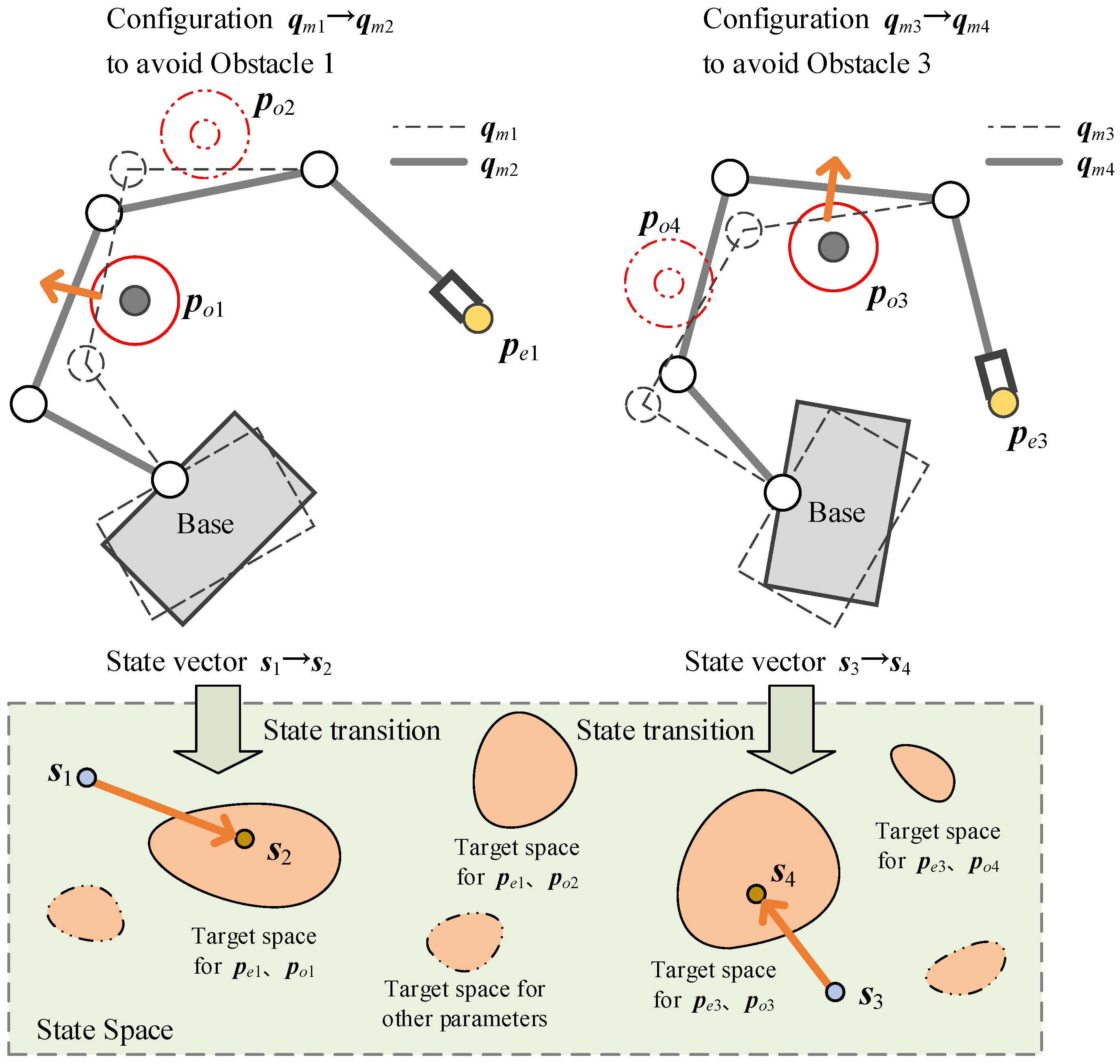
Secondly, the manipulator configurations and the end-effector positions are changeable for different scenarios or tasks. The RL agent needs to simultaneously learn a null-space policy for the changes of obstacle position, end-effector position and manipulator configuration. However, in practical applications, the possible obstacle positions are independent of the end-effector positions, which leads to the distribution discontinuity of the target state space in the whole state space, as shown in Figure 7. If the number of training samples is insufficient, it is easy to fall into the local optimum, which greatly reduces the policy’s performance. To this end, we design the adjustment strategies for the end-effector positions and the manipulator configuration for different training stages:
(a)
Specify the maximum number of training episode n ep _ max , the cumulative reward threshold R s , and an initial manipulator configuration q m 0 ;
(b)
Calculate the end-effector position x e by forward kinematics according to q m 0 ;
(c)
Start current episode under the condition of the unchanged x e to sample the trajectory of the space robot in null-space, and learn the obstacle-avoidance policy in null space by the SAC training pipeline;
(d)
If the cumulative reward in this episode is R t > R s , which means the space robot has learned an available policy under the condition of the end-effector position x e , then let q m 0 q m 0 + Δ q m 0 , where Δ q m 0 is a random configuration-changing vector. Otherwise, skip this step.
(e)
Turn to (b) for the next episode, until reaching n ep _ max .
In addition, we also use automating entropy adjustment strategy [37] to update α automatically for Equation (11):
J α = E a π θ α log π θ a | s α H ¯
α α ε · α J α
where J α is the objective function to update α , H ¯ is the specified target entropy value, ε is the scale factor. As the training progresses, α will be gradually decreased to make H · approach the target entropy value H ¯ . Therefore, the randomness of actions will be greater at the initial stage of training to expand the action exploration space and increase the possibility of searching for better policy. Then the randomness will be gradually reduced over the training process to ensure the convergence.
Combining all the above training strategies, the final training process is shown in the following Algorithm 1:
Algorithm 1: The training strategy for null-space obstacle avoidance of space robot.
Actuators 12 00069 i001

4. Simulation and Discussion

In order to verify the effectiveness of the motion planning method proposed in this paper, we designed the task scenario for a space robot and conducted the numerical simulation experiments. Then, we discussed the experimental results. All simulations were run on a computer with Intel i9-10900X 3.70 GHz CPU, Gigabyte X299-WU8 motherboard and four 16 GB Samsung DDR4 RAMs.

4.1. Simulation Scenario

For better display, we take a planar space robot with a floating base and a 3-DOF manipulator to verify our method, where the end-effector tracks the position so that the robot has a single redundant degree. The schematic diagram is shown in Figure 8, and the Denavit–Hartenberg (D-H) parameters and dynamic parameters are shown in Table 1 and Table 2, respectively. The constraints are listed in Table 3.
The simulation environment is developed by PyGame on OpenAI Gym, which is shown in Figure 9. The initial base position, orientation and manipulator configuration are set at p b 0 = [ 0.2 , 0 ] T ( m ) , r b 0 = 0 ° and q m 0 = [ 45 , 90 , 45 ] T ( ° ) respectively. Several obstacles with radius r o = 0.005 ( m ) and safe distance d s = 0.02 ( m ) are positioned randomly at p o 1 , p o 2 , , p o k in the scenario ( k = 2 in Figure 9). The space robot needs to avoid these obstacles at a safe distance d s while tracking the predetermined end-effector trajectory to the target position p t .

4.2. Training Process

We trained the RL agent with the hyperparameters in Table 4 to validate our null-space obstacle-avoidance method. As a comparison, we conducted two cases of training strategy: one is the curriculum learning strategy (Algorithm 1) proposed in Section 3.3, another is the common strategy, which takes the random initial manipulator configuration for each episode.
As Figure 4 shows, the SAC networks are composed of MLP fully connected layers. The policy network has an input layer with 14 nodes (the dimension of the state vector s t ), an output layer with 3 nodes (the dimension of the action vector a t ) and 256 hidden layers with 256 nodes. Each Q-networks has an input layer with 17 nodes (the dimension of s t and a t ), an output layer with 1 node, and 256 hidden layers with 256 nodes. All the nodes use ReLU for the activation function.
The training process went through 600 epochs, and each epoch contains 20 episodes, where an episode lasts 600 timesteps at most. Once the distance between the obstacle and the manipulator is greater than the safe distance or the manipulator collides with the obstacle, the episode will be terminated. If the distance between the links and the obstacles is greater than d s or less than r s , or the moving time elapses over 600 timesteps, the episode will terminate and come to the next episode until the current epoch ends. A performance test of 20 episodes is set between each epoch to verify the learning effect so far. The test results of the average, minimum and maximum accumulated rewards after each epoch for the above two training cases are shown in Figure 10.
It can be seen from Figure 10a that using our strategy, the cumulative reward is gradually converged after 300 epochs, and the difference between the maximum and minimum values is reducing, indicating that a relatively stable null-space obstacle-avoidance policy has been learned. In Figure 10b, as the training proceeds, the average and minimum of the cumulative reward fluctuate greatly all the time, showing that the performance is poor in the test, which cannot achieve effective obstacle avoidance under some initial manipulator configurations.
Figure 10c compares the average cumulative reward curves of the two training cases. We can see that the average cumulative reward of our method is temporarily lower in the initial training stage compared with the random initial configuration strategy; however, in the middle and late stages, the curve of our method is consistently higher than the latter. This is mainly because in the initial stage, our method tried to explore the policy for different obstacle positions under a fixed initial configuration. In other words, we restricted the target state space as well as the to-be-searched state space. Although there were many failed attempts, the RL agent learned the policy of reaching into the target state space from its edge under the specified initial configuration. After that, it gradually switched to other initial configurations to generalize the policy. Therefore, we can see that the test curve fluctuates to a certain extent after each switching of the initial configuration, indicating that the RL agent is carrying out the adaptive learning for the changed initial configuration. As for the random initial configuration strategy, each episode simultaneously generated the random initial configuration and obstacle position, resulting in the catastrophic expansion of the to-be-explored state space. The RL agent was trained with insufficient available samples, which obtained unstable test results. Figure 10d compares the obstacle-avoidance success rates of the two training cases. We define a successful obstacle avoidance as the minimum distance between the obstacle and each component of the space robot being greater than safety distance d s through the space robot’s motion within 600 timesteps. Therefore, it is considered a failure if any component collides with the obstacle, or the minimum distance is not greater than d s after 600 timesteps. From Figure 10d, we can also see a trend similar to that in Figure 10c as mentioned above. Finally, the success rate of our method converges to about 90%, while the success rate of random initial configuration strategy is about 83%, which is slightly lower than our method.

4.3. Results Discussion

4.3.1. Training Results

Figure 11 shows the null-space obstacle-avoidance motion of the space robot for different numbers of obstacles by the learned RL agent. The color in the figure gradually deepens over time so that the moving trajectory of the space robot can be seen intuitively. In the initial state, the distance between the obstacle and the links are less than the safety distance d s . Driven by the learned RL agent, the manipulator moved in the direction away from the safety boundary of the obstacle until the distance was greater than d s , then gradually stopped moving. During this process, the pose of the base changed slightly due to the motion coupling relationship between the base and the manipulator. However, the position of the end-effector did not change, which proves the null-space obstacle-avoidance characteristic of our method.
It can be seen from the simulation that our method has no limit to the number of obstacles. Although the RL agent was trained on a single-obstacle scenario, it is still applicable for scenarios with two or more obstacles. In addition, by combining with the end-effector trajectory generation strategy, it can achieve the high-required end-effector trajectory tracking task and obstacle avoidance in an unstructured dynamic environment simultaneously, as Section 4.3.3 shows.

4.3.2. Performance of Obstacle Avoidance

When performing tasks, the space robot needs to carry different loads, which are usually grasped by the end-effector or placed in specific storage areas of the base, resulting in mass distribution changes. Since the free-floating characteristic of the base, the different mass distribution will change the coupling degree between the base and the manipulator so that the original strategy cannot adapt to the changed dynamic nature of the robot, which is still a challenge faced by many planning and control methods for space robot.
To illustrate the robustness to payload mass change of our method, we used the above learned RL agent without modification to test the performance in different mass distributions. We set up 20 groups to test the effect of mass changes on the obstacle avoidance performance, where 10 groups for different base mass (from 100 kg to 1000 kg), and 10 groups for different end-effector mass (from 50 kg to 500 kg). Each group contained 100 obstacle avoidance tests. After a group was completed, we recorded the success rate of obstacle avoidance and the cumulative reward obtained by the RL agent. The results are shown in Figure 12.
As can be seen from Figure 12a, under the conditions of different base mass, the average success rate of the RL agents in null-space obstacle avoidance is 91.2%, and the cumulative reward is about −130, which is basically the same as the test results in the later training stage (the cumulative reward curve after 300 epochs in Figure 10a, indicating that base mass change has little effect on obstacle-avoidance performance. From Figure 12b, it can be seen that the average success rate is 89.3%, and the success rate decreases slightly with the increasing of the end-effector mass, while the changing trend of the cumulative reward is not obvious, indicating that the end-effector mass change also has little influence on the obstacle avoidance performance. Since the mass of the load is generally not greater than the base, it can be considered that our method has good robustness to the load changes according to the test results, which can meet the needs of practical tasks.
It should be pointed out that there is about a 10% failure rate in the above tests. They are caused by the loss of single directional motion capability, which comes from the strict null-space constraint, while not being caused by our method. Figure 13 shows a typical failure case, where an obstacle is placed near Link 2. Due to the restriction of the null-space constraint, Link 2 lost the ability to move upward to leave the obstacle’s safe distance border. In fact, no matter how the RL agent drove the space robot, Link 2 was always within the safe distance, or even closer to the obstacle such that the collision occurred. Therefore, in these cases, obstacle avoidance is impossible unless the end-effector’s positions are allowed to change; however, it is beyond the scope of the premises in this paper. We consider relaxing the strong constraint of null-space motion to solve this problem in later research.
Considering the null-space motion constraint, we did not compare our method with the conventional obstacle-avoidance motion planning methods, such as PRM and RRT, because they are difficult to meet the precondition of keeping the end-effector’s position unchanged during obstacle avoidance. Instead, we tested the common method GPM for null-space motion in the above simulation scenario with the same computer and programming language. We tested 500 episodes, where the initial manipulator configuration and obstacle position are randomly generated for each episode. We observed the effect of GPM and our method, respectively, in each episode and recorded the success rate of obstacle avoidance, as well as the average time to generate ϕ ˙ at each timestep. The results are shown in Table 5. It can be seen from the test results that the success rates of the two methods are the same, while neither of them reaches 100%. As mentioned in the previous paragraph, it was caused by the random generation of the initial manipulator configuration and obstacle position for which, in some cases, it is impossible to avoid the obstacle without changing the end-effector’s position, such as in Figure 13. In fact, both methods achieved the same 457 successful episodes, and the other 43 episodes failed unless the end-effector’s position was changed. It manifests that the two methods are at a nearly equivalent level for null-space obstacle avoidance. However, our method saves nearly 68% of the computation time compared to GPM. This is because our method obtains action values directly from the learned policy network, while the GPM computation relies on the iterative computation of the kinematics of the space robot, which consumes a lot of time.

4.3.3. Application in Dynamic Environment

Further, we tested the performance of our method in dynamic environments. We applied the learned RL agent without modification to the unstructured dynamic scenario with the following two conditions: (1) the end-effector needs to move along a predetermined trajectory; and (2) there are movable obstacles in the scenario that need to be avoided. In this scenario, the initial configuration of the space robot, the target position of the end-effector, as well as the initial and target position of the obstacle, are randomly generated.
Figure 14 shows the scenario settings of the simulation, with the initial base position p b 0 = [ 0.2 , 0 ] T ( m ) , initial base orientation r b 0 = 0 ° and initial configuration of the manipulator q m 0 = [ 20 , 130 , 140 ] T ( ° ) . The end-effector moved linearly from the initial position p e _ start = [ 0.004 , 0.010 ] T ( m ) to the target position p e _ target = [ 0.076 , 0.070 ] T ( m ) at the trapezoidal velocity profile with parabolic blends. There was an obstacle moving linearly in the scenario, from the initial position p o _ start = [ 0.094 , 0.100 ] T ( m ) to the target position p o _ target = [ 0.023 , 0.010 ] T ( m ) ; the motion curve is shown in Figure 15. In this case, the space robot moved directly according to the joint trajectory calculated by inverse kinematics without obstacle avoidance, then Link 1 and Link 2 broke through the obstacle’s safe distance border d s = 0.02 ( m ) successively, as shown in Figure 16. In detail, Figure 17 shows the distance curve between the obstacle and Link 1/Link 2 over time. It can be seen from the figure that the distance between Link 1 and Link 2 was less than the safe distance with 11.9 s, since Link 2 collided with the obstacle at 27.5 s. Obviously, it was a failed task.
We tested the same task with our method. In this case, the motion trajectory of the space robot is shown in Figure 18. As can be seen from the figure, the end-effector moved along the desired linear trajectory, while the RL agent actively drove Joint 2 and Link 2 to avoid the obstacle. Figure 19 shows the distance curve from the obstacle to Link 1/Link 2 by our method. In the initial stage, the distance curve is basically the same as Figure 17. The difference comes after 11.9s. Under the control of the RL agent, the distance between the obstacle and Link 1/Link 2 was kept at the safe distance until the obstacle was far away from Link 1 at 21.2 s, while still maintaining the safe distance from Link 2. Figure 20 compares the end-effector’s real trajectory by our method with the desired trajectory required by the task. In this figure, the real trajectory almost completely coincides with the desired trajectory, indicating that the obstacle-avoidance motion component strictly followed the null-space constraint, having no effect on the motion of the end-effector.
The simulation results demonstrate the effectiveness and adaptability to a dynamic unstructured environment of our proposed RL-based null-space obstacle-avoidance method. It also shows that our motion planning framework has good extensibility, which can be combined with different end-effector trajectory generators to perform more complex and no-collision manipulation tasks.

5. Conclusions

In this paper, a new obstacle-avoidance motion planning method for redundant space robots via reinforcement learning is proposed. Utilizing the redundant characteristics of the space robot, this method constructs an obstacle-avoidance motion planning framework, which introduces RL into null-space motion to realize reactive obstacle avoidance without changing the end-effector’s predetermined trajectory. Then, the proposed RL agent model as well as the training strategy for null-space obstacle avoidance is combined to the framework, which enables our method to have good adaptability to unstructured dynamic environments. The simulation results show that our method can avoid the stationary/moving obstacles steadily and effectively with sufficient computational efficiency, as well as having no need to retrain for the changes of obstacle number or motion states in the dynamic environment. Our method has good robustness to the space robot’s load mass, which is an important case to be considered in the practical application of space robot methods. We prove the advantages of our method in this aspect through a large number of tests. In addition, the simulation results also demonstrate the openness and extensibility of our method, which can be easily combined with the end-effector trajectory generation strategies, simultaneously realizing the complex motion tracking of the end-effector and the obstacle avoidance of the links for trajectory focused tasks.
In order to apply our method to real scenarios, the following steps need to be implemented: firstly, obtain the relatively accurate kinematics and dynamic parameters of the space robot so that the simulation environment can reliably simulate the real motion response in the space environment; secondly, train the RL agent according to the proposed strategy in the simulation environment built by the ground computer; thirdly, deploy the trained RL agent program to the control computer, which is launched into orbit with the space robot; finally, start this program when the space robot performs on-orbit operation tasks, where the joint angle and velocity come from the joint sensor embedded in the manipulator, and the obstacle information depends on the measurement results from the visual sensor so that the necessary state value is provided for the RL agent to realize null-space obstacle avoidance. Our method mainly consumes hardware resources in the ground training stage. After training, the RL agent can be executed without excessive hardware conditions, so it can be easily deployed to the control computer of the space robot.
It should be pointed out that null-space motion cannot guarantee the absolute obstacle-avoidance capability of the space robot in the full range of its workspace. Specifically, the links of the space robot may lose single directional motion capability by the null-space constraint such that it cannot avoid the obstacle in this direction unless the end-effector is no longer restricted to following the predetermined trajectory. Therefore, under the premise of the null-space constraint, the success rate of obstacle avoidance cannot reach 100% for random obstacles. For this situation, we need to allow the RL agent to relax the null-space constraint of tracking the end-effector’s predetermined trajectory when necessary so that once the obstacle’s motion exceeds the coping ability of null-space obstacle avoidance, the RL agent can still ensure the safety of the space robot. We will solve this problem in future research so as to further improve the performance of obstacle avoidance.

Author Contributions

Conceptualization, Z.H. and G.C.; methodology, Z.H.; software, Z.H. and Y.S.; validation, Z.H., Y.S. and R.W.; formal analysis, G.C. and C.L.; investigation, Z.H.; resources, C.L. and L.Z.; data curation, L.Z.; writing—original draft preparation, Z.H.; writing—review and editing, G.C.; visualization, Y.S.; supervision, R.W.; project administration, G.C.; funding acquisition, G.C. and C.L. All authors have read and agreed to the published version of the manuscript.

Funding

This research is supported by BUPT Action Plan to Enhance Capacity for Scientific and Technological Innovation (No. 2021XD-A10-1), BUPT Excellent Ph.D. Students Foundation (CX2021119), National Natural Science Foundation of China (No. 62173044, 61903354) and Science and Technology Foundation of State Key Laboratory (No. 19KY1208).

Institutional Review Board Statement

Not applicable.

Informed Consent Statement

Not applicable.

Data Availability Statement

Not applicable.

Conflicts of Interest

The authors declare no conflict of interest.

Abbreviations

The following abbreviations are used in this manuscript:
RLReinforcement learning
SACSoft actor–critic
D-H parameterDenavit-Hartenberg parameter

References

  1. Xue, Z.; Liu, J.; Wu, C.; Tong, Y. Review of In-Space Assembly Technologies. Chin. J. Aeronaut. 2021, 34, 21–47. [Google Scholar] [CrossRef]
  2. Moghaddam, B.M.; Chhabra, R. On the guidance, navigation and control of in-orbit space robotic missions: A survey and prospective vision. Acta Astronaut. 2021, 184, 70–100. [Google Scholar] [CrossRef]
  3. Dai, Y.; Xiang, C.; Zhang, Y.; Jiang, Y.; Qu, W.; Zhang, Q. A Review of Spatial Robotic Arm Trajectory Planning. Aerospace 2022, 9, 361. [Google Scholar] [CrossRef]
  4. Lozano-Pérez, T.; Wesley, M.A. An Algorithm for Planning Collision-Free Paths among Polyhedral Obstacles. Commun. ACM 1979, 22, 560–570. [Google Scholar] [CrossRef]
  5. Canny, J.; Donald, B. Simplified Voronoi Diagrams. Discret. Comput. Geom. 1988, 3, 219–236. [Google Scholar] [CrossRef]
  6. Kavraki, L.E.; Svestka, P.; Latombe, J.C.; Overmars, M.H. Probabilistic Roadmaps for Path Planning in High-Dimensional Configuration Spaces. IEEE Trans. Robot. Autom. 1996, 12, 566–580. [Google Scholar] [CrossRef]
  7. Kuffner, J.J.; LaValle, S.M. RRT-Connect: An Efficient Approach to Single-Query Path Planning. In Proceedings of the 2000 IEEE International Conference on Robotics and Automation, San Francisco, CA, USA, 24–28 April 2000; Volume 2, pp. 995–1001. [Google Scholar]
  8. Li, F.; Huang, Z.; Xu, L. Path Planning of 6-DOF Venipuncture Robot Arm Based on Improved A-Star and Collision Detection Algorithms. In Proceedings of the 2019 IEEE International Conference on Robotics and Biomimetics, Dali, China, 6–8 December 2019; pp. 2971–2976. [Google Scholar]
  9. Khatib, O. Real-Time Obstacle Avoidance for Manipulators and Mobile Robots. In Proceedings of the 1985 IEEE International Conference on Robotics and Automation Proceedings, St. Louis, MO, USA, 25–28 March 1985; Volume 2, pp. 500–505. [Google Scholar]
  10. Maciejewski, A.A.; Klein, C.A. Obstacle Avoidance for Kinematically Redundant Manipulators in Dynamically Varying Environments. Int. J. Robot. Res. 1985, 4, 109–117. [Google Scholar] [CrossRef]
  11. Kim, J.; Khosla, P.K. Real-Time Obstacle Avoidance Using Harmonic Potential Functions. IEEE Trans. Robot. Autom. 1992, 8, 338–349. [Google Scholar] [CrossRef]
  12. Wang, W.; Zhu, M.; Wang, X.; He, S.; He, J.; Xu, Z. An Improved Artificial Potential Field Method of Trajectory Planning and Obstacle Avoidance for Redundant Manipulators. Int. J. Adv. Robot. Syst. 2018, 15, 1729881418799562. [Google Scholar] [CrossRef]
  13. Wan, J.; Yao, J.; Wu, H. A Weighted Gradient Projection Method for Inverse Kinematics of Redundant Manipulators Considering Multiple Performance Criteria. Stroj. Vestn. J. Mech. Eng. 2018, 64, 475–488. [Google Scholar]
  14. Zhang, X.; Fan, B.; Wang, C.; Cheng, X. An Improved Weighted Gradient Projection Method for Inverse Kinematics of Redundant Surgical Manipulators. Sensors 2021, 21, 7362. [Google Scholar] [CrossRef]
  15. Guo, Z.Y.; Hsia, T.C. Joint Trajectory Generation for Redundant Robots in an Environment with Obstacles. J. Robot. Syst. 1993, 10, 199–215. [Google Scholar] [CrossRef]
  16. Haviland, J.; Corke, P. NEO: A Novel Expeditious Optimisation Algorithm for Reactive Motion Control of Manipulators. IEEE Robot. Autom. Lett. 2021, 6, 1043–1050. [Google Scholar] [CrossRef]
  17. Mu, Z.; Yang, Y.; Xu, W.; Gao, X.; Xue, L. Collision-Free Trajectory Planning of Redundant Space Manipulators Based on Pseudo-Distance. In Proceedings of the 11th World Congress on Intelligent Control and Automation, Shenyang, China, 29 June–4 July 2014; pp. 5232–5237. [Google Scholar]
  18. Hu, T.; Wang, T.; Li, J.; Qian, W. Gradient Projection of Weighted Jacobian Matrix Method for Inverse Kinematics of a Space Robot With a Controlled-Floating Base. Dyn. Syst. Meas. Control 2017, 139, 051013. [Google Scholar] [CrossRef]
  19. Wang, M.; Luo, J.; Walter, U. A Non-Linear Model Predictive Controller with Obstacle Avoidance for a Space Robot. Adv. Space Res. 2016, 57, 1737–1746. [Google Scholar] [CrossRef]
  20. Ni, S.; Chen, W.; Ju, H.; Chen, T. Coordinated Trajectory Planning of a Dual-Arm Space Robot with Multiple Avoidance Constraints. Acta Astron. 2022, 195, 379–391. [Google Scholar] [CrossRef]
  21. Rybus, T.; Wojtunik, M.; Basmadji, F.L. Optimal Collision-Free Path Planning of a Free-Floating Space Robot Using Spline-Based Trajectories. Acta Astron. 2022, 190, 395–408. [Google Scholar] [CrossRef]
  22. Lillicrap, T.P.; Hunt, J.J.; Pritzel, A.; Heess, N.; Erez, T.; Tassa, Y.; Silver, D.; Wierstra, D. Continuous Control with Deep Reinforcement Learning. arXiv 2015, arXiv:1509.02971. [Google Scholar]
  23. Cai, M.; Hasanbeig, M.; Xiao, S.; Abate, A.; Kan, Z. Modular Deep Reinforcement Learning for Continuous Motion Planning With Temporal Logic. IEEE Robot. Autom. Lett. 2021, 6, 7973–7980. [Google Scholar] [CrossRef]
  24. Fujimoto, S.; Hoof, H.; Meger, D. Addressing Function Approximation Error in Actor-Critic Methods. In Proceedings of the International Conference on Machine Learning, Stockholm, Sweden, 10–15 July 2018; pp. 1587–1596. [Google Scholar]
  25. Schulman, J.; Wolski, F.; Dhariwal, P.; Radford, A.; Klimov, O. Proximal Policy Optimization Algorithms. arXiv 2017, arXiv:1707.06347. [Google Scholar]
  26. Haarnoja, T.; Zhou, A.; Abbeel, P.; Levine, S. Soft Actor-Critic: Off-Policy Maximum Entropy Deep Reinforcement Learning with a Stochastic Actor. In Proceedings of the International Conference on Machine Learning, Stockholm, Sweden, 10–15 July 2018; pp. 1861–1870. [Google Scholar]
  27. Andrychowicz, M.; Wolski, F.; Ray, A.; Schneider, J.; Fong, R.; Welinder, P.; McGrew, B.; Tobin, J.; Abbeel, P.; Zaremba, W. Hindsight Experience Replay. In Proceedings of the 31st International Conference on Neural Information Processing Systems, Long Beach, CA, USA, 4–9 December 2017; pp. 5055–5065. [Google Scholar]
  28. Sangiovanni, B.; Incremona, G.P.; Piastra, M.; Ferrara, A. Self-Configuring Robot Path Planning with Obstacle Avoidance via Deep Reinforcement Learning. IEEE Control. Syst. Lett. 2021, 5, 397–402. [Google Scholar] [CrossRef]
  29. Tipaldi, M.; Iervolino, R.; Massenio, P.R. Reinforcement Learning in Spacecraft Control Applications: Advances, Prospects, and Challenges. Annu. Rev. Control 2022, 54, 1–23. [Google Scholar] [CrossRef]
  30. Yan, C.; Zhang, Q.; Liu, Z.; Wang, X.; Liang, B. Control of Free-Floating Space Robots to Capture Targets Using Soft Q-Learning. In Proceedings of the 2018 IEEE International Conference on Robotics and Biomimetics, Kuala Lumpur, Malaysia, 12–15 December 2018; pp. 654–660. [Google Scholar]
  31. Du, D.; Zhou, Q.; Qi, N.; Wang, X.; Liu, Y. Learning to Control a Free-Floating Space Robot Using Deep Reinforcement Learning. In Proceedings of the 2019 IEEE International Conference on Unmanned Systems, Beijing, China, 17–19 October 2019; pp. 519–523. [Google Scholar]
  32. Wu, Y.; Yu, Z.; Li, C.; He, M.; Hua, B.; Chen, Z. Reinforcement Learning in Dual-Arm Trajectory Planning for a Free-Floating Space Robot. Aerosp. Sci. Technol. 2020, 98, 105657. [Google Scholar] [CrossRef]
  33. Wang, S.; Cao, Y.; Zheng, X.; Zhang, T. Collision-Free Trajectory Planning for a 6-DoF Free-Floating Space Robot via Hierarchical Decoupling Optimization. IEEE Robot. Autom. Lett. 2022, 7, 4953–4960. [Google Scholar] [CrossRef]
  34. Li, Y.; Li, D.; Zhu, W.; Sun, J.; Zhang, X.; Li, S. Constrained Motion Planning of 7-DOF Space Manipulator via Deep Reinforcement Learning Combined with Artificial Potential Field. Aerospace 2022, 9, 163. [Google Scholar] [CrossRef]
  35. Jia, Q.; Liu, Y.; Chen, G.; Sun, H. Maximum Load Path Planning for Space Manipulator in Point-to-Point Task. In Proceedings of the 2013 IEEE 8th Conference on Industrial Electronics and Applications, Melbourne, Australia, 19–21 June 2013; pp. 988–993. [Google Scholar]
  36. Shahid, A.A.; Piga, D.; Braghin, F.; Roveda, L. Continuous Control Actions Learning and Adaptation for Robotic Manipulation through Reinforcement Learning. Auton. Robot. 2022, 46, 483–498. [Google Scholar] [CrossRef]
  37. Haarnoja, T.; Zhou, A.; Hartikainen, K.; Tucker, G.; Ha, S.; Tan, J.; Kumar, V.; Zhu, H.; Gupta, A.; Abbeel, P.; et al. Soft Actor-Critic Algorithms and Applications. arXiv 2019, arXiv:1812.05905. [Google Scholar]
Figure 1. Schematic diagram of space robot motion in unstructured environment.
Actuators 12 00069 g001
Figure 2. Motion planning framework for redundant space robot.
Actuators 12 00069 g002
Figure 3. The basic process of RL.
Actuators 12 00069 g003
Figure 4. SAC network structure for null-space obstacle avoidance.
Actuators 12 00069 g004
Figure 5. Schematic diagram of distance vector definition.
Actuators 12 00069 g005
Figure 6. Schematic diagram of obstacle position generation strategy.
Actuators 12 00069 g006
Figure 7. Schematic diagram of obstacle position, end-effector position and target state space distribution.
Actuators 12 00069 g007
Figure 8. Schematic diagram of the space robot.
Actuators 12 00069 g008
Figure 9. Simulation environment for planar space robot.
Actuators 12 00069 g009
Figure 10. The cumulative reward and success rate curves of two training cases.
Actuators 12 00069 g010aActuators 12 00069 g010b
Figure 11. Null-space obstacle-avoidance trajectory of the space robot.
Actuators 12 00069 g011
Figure 12. The performance of the RL agent in different mass distributions.
Actuators 12 00069 g012
Figure 13. A failure case in null-space obstacle avoidance.
Actuators 12 00069 g013
Figure 14. The scenario settings of the dynamic environment.
Actuators 12 00069 g014
Figure 15. The motion curve of the obstacle.
Actuators 12 00069 g015
Figure 16. The trajectory without obstacle avoidance of the space robot.
Actuators 12 00069 g016
Figure 17. The distance curve from the obstacle to the links without obstacle avoidance.
Actuators 12 00069 g017
Figure 18. The obstacle-avoidance trajectory of the space robot by our method.
Actuators 12 00069 g018
Figure 19. The distance curve from the obstacle to the links by our method.
Actuators 12 00069 g019
Figure 20. The motion curve of the end-effector by our method.
Actuators 12 00069 g020
Table 1. D-H parameters of the space robot.
Component Frame a i 1 ( m ) α i 1 ( ° ) d i ( m ) θ i ( ° )
b 0 0.05 000
0 1 000 q m 1
1 2 0.1 00 q m 2
2 3 0.1 00 q m 3
3 e 0.1 000
Table 2. Dynamic parameters of the space robot.
ComponentMass
m ( kg )
Centroid p ci ( m )
p x , p y , p z
Inertia Tensor I ci ( kg · m 2 )
I xx , I yy , I zz , I xy , I xz , I yz
Base500[0, 0, 0][20, 20, 20, 0, 0, 0]
Link110[0.25, 0, 0][0.00025, 0.8333, 0.8333, 0, 0, 0]
Link210[0.25, 0, 0][0.00025, 0.8333, 0.8333, 0, 0, 0]
Link310[0.25, 0, 0][0.00025, 0.8333, 0.8333, 0, 0, 0]
End_effector10[0.25, 0, 0][0.00025, 0.8333, 0.8333, 0, 0, 0]
Table 3. Constraint condition of the space robot.
ItemValueItemValue
q m 1 [ 120 ° , 120 ° ] ϕ ˙ 1 [ 1 ° , 1 ° ]
q m 2 [ 160 ° , 160 ° ] ϕ ˙ 2 [ 1 ° , 1 ° ]
q m 3 [ 160 ° , 160 ° ] ϕ ˙ 3 [ 1 ° , 1 ° ]
Table 4. Hyperparameters of the RL agent for training.
HyperparameterValueHyperparameterValue
Learning rate0.001Obstacle number k1
Discount factor γ 0.99Reward threshold R s −50
Target entropy H ¯ −4Scale factor ε 1
Temperature α 0.2Configuration change Δ q m 0 ( 15 ° , + 15 ° )
Replay buffer size 1 × 10 5 Reward parameter λ 1 10
Batch size100Reward parameter λ 2 0.3
Max length of an episode600Reward parameter r c −100
Table 5. Performance comparison of GPM and our method.
ComparisonGPMOur Method
Success Rate91.4%91.4%
Calculating Time2.367 ms0.753 ms
Disclaimer/Publisher’s Note: The statements, opinions and data contained in all publications are solely those of the individual author(s) and contributor(s) and not of MDPI and/or the editor(s). MDPI and/or the editor(s) disclaim responsibility for any injury to people or property resulting from any ideas, methods, instructions or products referred to in the content.

