A Novel State Estimation Approach for Suspension System with Time-Varying and Unknown Noise Covariance

Abstract

In this paper, a novel state estimation approach based on the variational Bayesian adaptive Kalman filter (VBAKF) and road classification is proposed for a suspension system with time-varying and unknown noise covariance. Using the VB approach, the time-varying noise covariance can be inferred from the inverse-Wishart distribution and then optimized state estimation by the finite sampling posterior probability distribution function (PDF) of noise covariance and backward Kalman smoothing. In addition, a new road classification algorithm based on multi-objective optimization and the linear classifier is proposed to identify the unknown noise covariance. Simulation results for a suspension model with time-varying and unknown noise covariance show that the proposed approach has a higher performance in state estimation accuracy than other filters.

1. Introduction

As one of the components of the vehicle, the dynamic response of the suspension system plays an important role in the overall performance of the vehicle. Therefore, in order to improve the ride comfort of the vehicle, many suspension control methods have been proposed based on state measurement [1,2,3]. However, the measurement results are subject to sensor uncertainty and unknown road conditions. As a result, the system state variables cannot be accurately measured. The Kalman filter is a recursive state space model based on optimal estimation that is widely used for dynamic system state estimation [4,5,6]. such as localization, tracking and control. In the suspension state estimation process, filter performance mainly depends on the accuracy of the noise covariance, and an inaccurate noise covariance will lead to estimation errors or even filter divergence [7]. The actual vehicle driving conditions tend to vary with time and are unknown to the road level, resulting in the process noise covariance matrix (PNCM) and the measurement noise covariance matrix (MNCM) having the same characteristics.

To estimate states with time-varying and unknown noise covariance, many adaptive Kalman filter (AKF) methods have been developed, mainly including the following categories: covariance matching, correlation, maximum likelihood and Bayesian [8]. In addition to the adaptive Kalman filter, another well-known filter design for model uncertainty is the robust Kalman filter, which is equivalent to solving a minimax problem, i.e., selecting the worst model in a given uncertain fuzzy set and then designing the corresponding optimal filter [9,10,11]. However, the idea of the robust strategy is to first find the worst case of the model at the current time, which is the boundary of the uncertain parameters that need to be known. This can of course be achieved statistically by repeated experiments in a single scenario but seems difficult to achieve for time-varying and unknown noise covariances. In addition, robust strategies may be too conservative in terms of the optimal solution obtained, given the convergence performance of the filter.

The covariance matching method uses a sliding window of the innovation sequence to approximate the true noise covariance. Due to its simplicity of implementation, it is widely used in many works [12,13,14]. However, the estimation accuracy of this method is closely related to the window size and requires a priori knowledge of the innovation sequence. The basic idea of the correlation method is to correlate the system output or the autocorrelation function of the innovation sequence with the unknown system parameters [15]. In the literature [16], the correlation method is used to estimate the MNCM and to identify the PNCM based on the road classification method. However, the correlation method is mainly applicable to constant coefficient systems, which requires the assumption that the system performance is in steady state. The maximum likelihood estimation method defines a probability density function with the unknown parameters as independent variables, usually called the likelihood function, and solves for its extreme value points. Some improved maximum likelihood estimation methods can be found in [17,18,19]. In [19], the Maximum Likelihood Principle (MLP) is used to estimate the unknown noise of nonlinear dynamic systems, and a new expectation maximization technique is proposed to iteratively optimize the computational process of the MLP. However, this method is still not suitable for estimating unknown noise parameters with time-varying properties. The Bayesian method uses the Bayesian formula to iteratively solve the posterior PDF of the state and unknown parameters. For some complex probability distributions, variational inference can be combined to simplify the computational process [20]. Recent studies have further reduced the estimation error by combining the Kalman smoother with variational Bayes [21,22,23]. However, their output ignores the smoothed data series and approximates the prior of the covariance matrix with individual data values, which may result in the estimation of the noise covariance falling into a local optimum.

For the existing VBAKF methods, the noise covariance estimation process relies heavily on the parameter selection of the approximate distribution. The convergence of the iterative process is accelerated by selecting a suitable conjugate prior distribution and assuming that the nominal values of PNCM and MNCM are known. However, for unknown road conditions, the nominal values of the noise covariance corresponding to different road levels are obviously not fixed. To solve the above problem, this paper proposes a novel state estimation approach based on VBAKF and road classification to estimate the suspension state with time-varying and unknown noise covariance. In the proposed approach, the suspension state estimation process is still basically completed by VBAKF by assuming that the conjugate prior distribution of the matrix is approximately the inverse-Wishart (IW) distribution. However, in order to make full use of the valid data in the iterative process and to improve the accuracy of the state estimation, a heuristic propagation method is used to finitely sample the posterior noise variance, and the propagated estimated samples are folded. Then, to overcome the disadvantage that the traditional VBAKF cannot cope well with the unknown road gradient, a road classification method combining multi-objective optimization and the suspension dynamic response linear classifier is proposed.

In summary, the following contributions are made in this thesis:

• For the estimation of the suspension state with time-varying and unknown noise covariance, a novel state estimation approach based on a variational Bayesian adaptive Kalman filter and road classification is proposed.
• Using the variational Bayesian approach, the time-varying noise covariance can be inferred from the inverse Wishart distribution; then, state estimation is optimized by finite sampling the posterior probability distribution function of the noise covariance and backward Kalman smoothing.
• To identify the unknown noise covariance, a new road classification algorithm based on multi-objective optimization and the linear classifier is proposed.

The rest of the paper is structured as follows. In the next section, the plant equations of the quarter-car vehicle model are presented, as well as the standard Kalman filter. Section 3 mainly introduces the novel state estimation approach for a suspension system with time-varying and unknown noise covariance. In Section 3.1, we introduce the variational Bayesian approach to approximate the time-varying noise covariance. Section 3.2 presents the proposed road classification algorithm. Then, in Section 4, some numerical experiments are provided. Finally, Section 5 concludes this article.

2. Problem Formulation

In order to simulate the complex dynamic characteristics of the suspension system, various complex suspension models have been proposed [24]. In this paper, the two-degree-of-freedom (2-DOF) linear suspension model is used to analyze the suspension dynamic response. The structure of the suspension model is shown in Figure 1.

According to Newton’s second law, the dynamic equations of the suspension system are given by (1) and (2):

$$\begin{array}{c}{m}_s {\ddot{z}}_s+k_s(z_s-z_u)+c_s({\dot{z}}_s-{\dot{z}}_u)=0\hfill \end{array}$$

(1)

$$\begin{array}{c}{m}_u {\ddot{z}}_u-k_s(z_s-z_u)-c_s({\dot{z}}_s-{\dot{z}}_u)+k_t(z_u-z_r)=0\hfill \end{array}$$

(2)

where $m_s$ and $m_u$ are the sprung mass and unsprung masses, $k_s$ and $k_t$ are the suspension spring stiffness and tyre stiffness, $c_s$ is the suspension damping.

When the system state, measurement output and disturbance vectors are respectively defined as follows:

$$x=\left[\begin{array}{c}{z}_s-z_u\\ z_u-z_r\\ {\dot{z}}_s\\ {\dot{z}}_u\end{array}\right],y=\left[\begin{array}{c}{\ddot{z}}_s\\ z_s-z_u\\ z_u-z_r\end{array}\right],w=\left[\begin{array}{c}{\dot{z}}_r\end{array}\right]$$

The equation of the continuous-time state space model can be written as

$$\begin{array}{cc}\hfill \dot{x}& =A_{c}x+B_{c}w\hfill \end{array}$$

(3)

$$\begin{array}{cc}\hfill y& =C_{c}x+v\hfill \end{array}$$

(4)

where x is the system state vector with the dimension of $d_x$, y is the system measurement vector with the dimension of $d_y$, and $A_c$, $B_c$, $C_c$ are the state space parameter matrix, which can be written as follows:

$$A_c=\left[\begin{array}{cccc}0& 0& 1& -1\\ 0& 0& 0& 1\\ \frac{k_s}{m_s}& 0& \frac{c_s}{m_s}& -\frac{c_s}{m_s}\\ -\frac{k_s}{m_u}& \frac{k_t}{m_u}& -\frac{c_s}{m_u}& \frac{c_s}{m_u}\end{array}\right],B_c=\left[\begin{array}{c}0\\ -1\\ 0\\ 0\end{array}\right],C_c=\left[\begin{array}{cccc}\frac{k_s}{m_s}& 0& \frac{c_s}{m_s}& -\frac{c_s}{m_s}\\ 1& 0& 0& 0\\ 0& 1& 0& 0\end{array}\right]$$

Using the zero-order hold with sampling period T, the discrete state space model can be obtained:

$$\begin{array}{cc}\hfill x_k& =A_d{x}_{k-1}+B_d{w}_{k-1}\hfill \end{array}$$

(5)

$$\begin{array}{cc}\hfill y_k& =C_d{x}_k+v_k\hfill \end{array}$$

(6)

$$\begin{array}{c}\hfill A_d=e^{A_{c}T},B_d={\int }_0^T{e}^{A_{c}s}{B}_{c}ds,C_d=C_c\end{array}$$

(7)

where k is the sampling discrete-time instant, while the process disturbance vector w and measurement noise vector v are defined as $w\sim \mathrm{N}\left(0,Q\right)$, $v\sim \mathrm{N}\left(0,R\right)$, respectively.

The basic idea of the standard Kalman filter is to solve for the optimal system state in the least squares sense and to estimate the state of the suspension system by state prediction (8) and state correction (9) iterative models.

• Predicting process:

$$\begin{array}{c}\hfill \left\{\begin{array}{c}{\widehat{x}}_{k|k-1}=A{\widehat{x}}_{k-1}\hfill \\ P_{k|k-1}=A{P}_{k-1}{A}^T+B{Q}_{k-1}{B}^T\hfill \end{array}\right.\end{array}$$

(8)

• Updating process:

$$\begin{array}{c}\hfill \left\{\begin{array}{c}{K}_k=P_{k|k-1}{C}^T{(C{P}_{k|k-1}{C}^T+R_k)}^{-1}\hfill \\ {\widehat{x}}_k={\widehat{x}}_{k|k-1}+K_k(y_k-C{\widehat{x}}_{k|k-1})\hfill \\ P_k=(I-K_{k}C)P_{k|k-1}\hfill \end{array}\right.\end{array}$$

(9)

where $\widehat{x}$ denotes the approximate estimate of x.

For the suspension system, the inaccurate PNCM (Q) and MNCM (R) tend to have both time-varying and unknown characteristics. The time-varying characteristic is that the covariance varies slowly with time, and the unknown characteristic is that the covariance has an unknown magnitude for different road levels.

3. Main Results

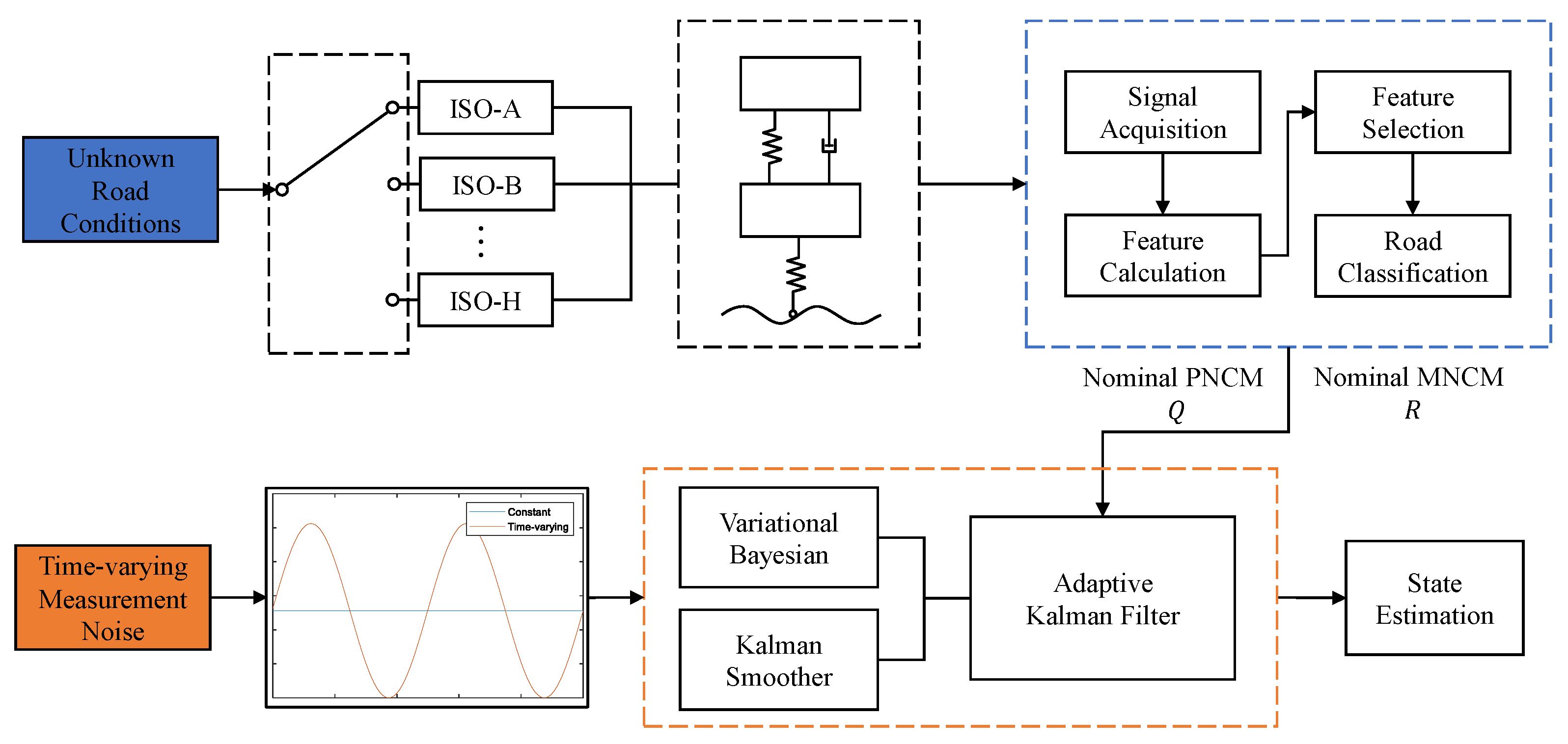
The overall flowchart of the proposed variable fractional Bayesian adaptive Kalman filter combined with road classification recognition for the suspension state estimator is shown in Figure 2. The sensor-induced time-varying observational noise differs from the conventional sense of a fixed constant value, and therefore a forward adaptive Kalman filter must be designed via a variational Bayesian to obtain estimates of the time-varying noise covariance matrices PNCM (Q) and MNCM (R). In addition, a backward propagating Kalman smoother can be combined with this to further improve the accuracy of the time-varying noise estimation. However, the application of a variational Bayesian filter requires a combination of a priori knowledge of the noise covariance matrices Q and R, i.e., nominal values. Therefore, based on the fact that the dynamic response of the suspension varies significantly on different road classes, a linear classifier can be used to identify the currently unknown road condition and finally obtain an accurate estimate of the suspension state. The specific process of applying VBAKF under time-varying noise covariance and unknown road level is further described in the following section.

3.1. Variational Bayes

According to Bayesian optimal filter theory, to obtain the state estimate $x_k$, the joint posterior PDF of $p(x_k,P_{k|k-1},R_k|y_{1:k})$ must first be solved. Formally, there are only approximate solutions to this PDF, and a well-known method for solving it is the VB approximation. Using the VB method, this posterior PDF can be expanded as follows:

$$\begin{array}{cc}\hfill p(x_k,P_{k|k-1},R_k|y_{1:k})& \approx q\left(x_k\right)q\left(P_{k|k-1}\right)q\left(R_k\right)\hfill \end{array}$$

(10)

where the optimal approximation $q(·)$ can be solved by minimizing the Kullback–Leibler (KL) divergence between the approximation distribution and the true joint posterior [25], that is,

$$\begin{array}{cc}\hfill & \mathrm{argmin}\mathrm{KL}\left[q\left(x_k\right)q\left(P_{k|k-1}\right)q\left(R_k\right)\right|\left|p(x_k,P_{k|k-1},R_k|y_{1:k})\right]\hfill \\ \hfill & =\int \int \int q\left(x_k\right)q\left(P_{k|k-1}\right)q\left(R_k\right)log\left(\frac{q\left(x_k\right)q\left(P_{k|k-1}\right)q\left(R_k\right)}{p(x_k,P_{k|k-1},R_k|y_{1:k})}\right)\hfill \\ \hfill & \mathrm{d}{x}_k\mathrm{d}{P}_{k|k-1}\mathrm{d}{R}_k\hfill \end{array}$$

(11)

Using the same variational Bayes calculation methods as in [26,27], the solution of (11) can be simplified to the following form:

$$\begin{array}{c}\hfill \left\{\begin{array}{c}q\left(x_k\right)\propto exp{\mathbb{E}}_{q(/x_k)}\left[logp(x_k,P_{k|k-1},R_k,y_{1:k})\right]\hfill \\ q\left(P_{k|k-1}\right)\propto exp{\mathbb{E}}_{q(/P_{k|k-1})}\left[logp(x_k,P_{k|k-1},R_k,y_{1:k})\right]\hfill \\ q\left(R_k\right)\propto exp{\mathbb{E}}_{q(/R_k)}\left[logp(x_k,P_{k|k-1},R_k,y_{1:k})\right]\hfill \end{array}\right.\end{array}$$

(12)

where $/x_k$ denotes the elements in $x_k,P_{k|k-1},R_k$ that are complementary to $x_k$, and $\mathbb{E}(/x_k)$ denotes taking expectation over $P_{k|k-1}$ and $R_k$. Next, only the joint PDF $p(x_k,$ $P_{k|k-1},R_k,y_{1:k})$ needs to be computed to approximate the posterior PDF $q\left(x_k\right)$, $q\left(P_{k|k-1}\right)$ and $q\left(R_k\right)$.

In the recursive model of KF (8) and (9), the filtering posterior PDF $p\left(x_k\right|y_{1:k-1})$ and $p\left(y_k\right|x_k)$ are approximated as Gaussian distributions.

$$\begin{array}{ccc}\hfill p\left(y_k\right|x_k)& \approx & \mathrm{N}(y_k;C{x}_k,R_k)\hfill \end{array}$$

(13)

$$\begin{array}{ccc}\hfill p\left(x_k\right|y_{1:k-1})& \approx & \mathrm{N}(x_k;{\widehat{x}}_{k|k-1},P_{k|k-1})\hfill \end{array}$$

(14)

In the theoretical framework of VB, the conjugate prior distribution of $P_{k|k-1}$, $R_k$ can be assumed to be the inverse Wishart distribution, because its prior distribution has the same functional form as the multivariate normal distribution [28], that is,

$$\begin{array}{ccc}\hfill p\left(P_{k|k-1}\right|y_{1:k-1})& =& \mathrm{IW}(P_{k|k-1};{\widehat{t}}_{k|k-1},{\widehat{T}}_{k|k-1})\hfill \end{array}$$

(15)

$$\begin{array}{ccc}\hfill p\left(R_k\right|y_{1:k-1})& =& \mathrm{IW}(R_k;{\widehat{u}}_{k|k-1},{\widehat{U}}_{k|k-1})\hfill \end{array}$$

(16)

where $\widehat{t}$ is a parameter representing the degrees of freedom of the IW distribution and $\widehat{T}$ denotes the scale parameter of the IW distribution, which must be positive definite. In addition, $\widehat{u}$ and $\widehat{U}$ have the same parametric meaning.

Considering that there are many constant terms in the inverse Wishart distribution and Gaussian distributions that do not affect the shape of the PDF that can be safely removed, the simplified density function can be written as

$$\begin{array}{c}\hfill \left\{\begin{array}{c}\mathrm{IW}(\mathsf{\Omega };\lambda ,\psi )\propto {\left|\mathsf{\Omega }\right|}^{-\frac{\lambda +d+1}{2}}exp\left[-\frac{1}{2}\mathrm{tr}\left(\psi {\mathsf{\Omega }}^{-1}\right)\right]\hfill \\ \mathrm{N}(x;\widehat{x},P)\propto {\left|P\right|}^{-\frac{1}{2}}exp\left[-\frac{1}{2}{(x-\widehat{x})}^T{P}^{-1}(x-\widehat{x})\right]\hfill \end{array}\right.\end{array}$$

(17)

where $\mathsf{\Omega }\triangleq \{P_{k|k-1},R_k\}$ denotes the noise covariance with the matrix dimension of $d_{\mathsf{\Omega }}\times d_{\mathsf{\Omega }}$, and $\mathrm{IW}(\mathsf{\Omega };\lambda ,\psi )$ denotes the IW distribution with the DOF parameter $\lambda$ and the inverse scale matrix $\psi$. The mean value of $\mathsf{\Omega }$ is

$$\begin{array}{c}\hfill \mathbb{E}\left(\mathsf{\Omega }\right)=\frac{\psi }{\lambda -d_{\mathsf{\Omega }}-1}\end{array}$$

(18)

The system state $x_k$ and the process error covariance matrix (PECM) $P_{k|k-1}$ refer only to the data at time $k-1$, and the measurement noises $v_k$ are independent random vectors. Thus, using the concept of conditional probabilities, the joint PDF $p(x_k,P_{k|k-1},R_k,y_{1:k})$ can be decomposed as follows:

$$\begin{array}{cc}\hfill p(x_k,P_{k|k-1},R_k,y_{1:k})=& p(y_k,x_k,P_{k|k-1},R_k|y_{1:k-1})p\left(y_{1:k-1}\right)\hfill \\ \hfill =& p\left(y_k\right|x_k)p\left(x_k\right|y_{1:k-1})p\left(P_{k|k-1}\right|y_{1:k-1})\hfill \\ \hfill & \times p\left(R_k\right|y_{1:k-1})p\left(y_{1:k-1}\right)\hfill \end{array}$$

(19)

Using (17) and (19), $logp(x_k,P_{k|k-1},R_k,y_{1:k})$ can be formulated as

$$\begin{array}{cc}\hfill & logp(x_k,P_{k|k-1},R_k,y_{1:k})\hfill \\ \hfill & =-\frac{1}{2}tr\left(\mathbb{E}\left[(x_k-{\widehat{x}}_{k|k-1}){(x_k-{\widehat{x}}_{k|k-1})}^T\right]P_{k|k-1}^{-1}\right)-\frac{1}{2}log\left|P_{k|k-1}\right|\hfill \\ \hfill & -\frac{1}{2}tr\left(\mathbb{E}\left[(y_k-C{x}_k){(y_k-C{x}_k)}^T\right]R_k^{-1}\right)-\frac{1}{2}log\left|R_k\right|\hfill \\ \hfill & -\frac{1}{2}\mathrm{tr}\left(\psi {\mathsf{\Omega }}^{-1}\right)-\frac{1}{2}(\lambda +d_{\mathsf{\Omega }}+1)log\left|\mathsf{\Omega }\right|+c\hfill \end{array}$$

(20)

Using (20), (12) can be referenced as follows:

$$\begin{array}{cc}\hfill logq\left(P_{k|k-1}\right)& ={\mathbb{E}}_{q(/P_{k|k-1}|y_{1:k})}\left[logp(x_k,{\mathsf{\Omega }}_k,y_{1:k})\right]\hfill \\ \hfill & =-\frac{1}{2}(t_{k|k-1}+d_x+2)log\left|P_{k|k-1}\right|\hfill \\ \hfill & -\frac{1}{2}tr\left[(T_{k|k-1}+A_k){P_{k|k-1}}^{-1}\right]+c_P\hfill \end{array}$$

(21)

$$\begin{array}{cc}\hfill logq\left(R_k\right)& ={\mathbb{E}}_{q(/R_k|y_{1:k})}\left[logp(x_k,{\mathsf{\Omega }}_k,y_{1:k})\right]\hfill \\ \hfill & =-\frac{1}{2}(u_{k|k-1}+d_y+2)log\left|R_k\right|\hfill \\ \hfill & -\frac{1}{2}tr\left[(U_{k|k-1}+B_k){R_k}^{-1}\right]+c_R\hfill \end{array}$$

(22)

where

$$\begin{array}{cc}\hfill A_k& =\mathbb{E}\left[(x_k-x_{k|k-1}){(x_k-x_{k|k-1})}^T\right]\hfill \\ \hfill & =({\widehat{x}}_k-x_{k|k-1}){({\widehat{x}}_k-x_{k|k-1})}^T+P_k\hfill \end{array}$$

(23)

$$\begin{array}{cc}\hfill B_k& =\mathbb{E}\left[(y_k-C{x}_k){(y_k-C{x}_k)}^T\right]\hfill \\ \hfill & =(y_k-C{\widehat{x}}_k){(y_k-C{\widehat{x}}_k)}^T+C{P}_k{C}^T\hfill \end{array}$$

(24)

From Equations (21) and (22), it can be seen that the posterior PDF at time k follows the functional form of the IW distribution. Furthermore, according to the Equations (15) and (16), the posterior PDF of $P_{k|k-1}$, $R_k$ has the following densities:

$$\begin{array}{ccc}\hfill q\left(P_{k|k-1}\right)& =& \mathrm{IW}(P_{k|k-1};{\widehat{t}}_{k|k},{\widehat{T}}_{k|k})\hfill \end{array}$$

(25)

$$\begin{array}{ccc}\hfill q\left(R_k\right)& =& \mathrm{IW}(R_k;{\widehat{u}}_{k|k},{\widehat{U}}_{k|k})\hfill \end{array}$$

(26)

By adjusting the elements of (21)–(26), the posterior PDF parameters in (25) and (26) can be updated as follows:

$$\left\{\begin{array}{c}\begin{array}{c}{\widehat{t}}_{k|k}={\widehat{t}}_{k|k-1}+1\hfill \\ {\widehat{T}}_{k|k}={\widehat{T}}_{k|k-1}+A_k\hfill \\ {\widehat{u}}_{k|k}={\widehat{u}}_{k|k-1}+1\hfill \\ {\widehat{U}}_{k|k}={\widehat{U}}_{k|k-1}+B_k\hfill \end{array}\hfill \end{array}\right.$$

(27)

Since the one-step approximation method cannot accurately estimate the distribution parameters of (27) PECM ($P_{k|k-1}$) and MNCN ($R_k$), the fixed-point iteration method must be used to find the optimal estimate. In addition, a heuristic parameter propagation method similar to [29] is used to iteratively update the approximate posterior PDF $q\left(P_{k|k-1}\right)$, $q\left(R_k\right)$, that is,

$$\left\{\begin{array}{c}\begin{array}{c}{\widehat{t}}_{k|k-1}={\rho }_P({\widehat{t}}_{k-1|k-1}-d_x-1)+d_x+1\hfill \\ {\widehat{T}}_{k|k-1}={\rho }_P{\widehat{T}}_{k-1|k-1}\hfill \\ {\widehat{u}}_{k|k-1}={\rho }_R({\widehat{u}}_{k-1|k-1}-d_y-1)+d_y+1\hfill \\ {\widehat{U}}_{k|k-1}={\rho }_R{\widehat{U}}_{k-1|k-1}\hfill \end{array}\hfill \end{array}\right.$$

(28)

where $\rho \in (0,1]$ is a forgetting factor value that reflects the time-varying fluctuation of the noise covariance, and $\rho =1$ indicates that the noise covariance is stable.

According to (18), the ith iteration estimates of PECM and MNCM can be expressed as the expected value of the IW distribution:

$$\begin{array}{cc}\hfill {\widehat{P}}_{k|k-1}^{\left(i\right)}& ={\widehat{T}}_{k|k}^{\left(i\right)}{({\widehat{t}}_{k|k}^{\left(i\right)}-n_x-1)}^{-1}\hfill \end{array}$$

(29)

$$\begin{array}{cc}\hfill {\widehat{R}}_k^{\left(i\right)}& ={\widehat{U}}_{k|k}^{\left(i\right)}{({\widehat{u}}_{k|k}^{\left(i\right)}-n_y-1)}^{-1}\hfill \end{array}$$

(30)

Using the $\delta$-function, the posterior PDF of MNCM can be assumed to be obtained by averaging over finite approximate solutions ${\left\{{\widehat{R}}^i\right\}}_{i=1}^N=\{{\widehat{R}}^1,{\widehat{R}}^2,\cdots ,{\widehat{R}}^N\}$ [30]. Thus, the posterior PDF $p\left(R\right|y_{1:k})$ can be represented in the following form:

$$\begin{array}{c}\hfill p\left(R_k\right|y_{1:k})\approx \sum _{i=1}^{N}p\left({\widehat{R}}_k^{\left(i\right)}\right|y_{1:k})\delta (R_k-{\widehat{R}}_k^{\left(i\right)})\end{array}$$

(31)

Using the Bayes rule, the calculation of $p\left({\widehat{R}}_k^{\left(i\right)}\right|y_{1:k})$ can be performed as follows:

$$\begin{array}{ccc}\hfill p\left({\widehat{R}}_k^{\left(i\right)}\right|y_{1:k})& =& p\left({\widehat{R}}_k^{\left(i\right)}\right|y_k,y_{1:k-1})\hfill \\ & =& \frac{p\left(y_k\right|{\widehat{R}}_k^{\left(i\right)},y_{1:k-1})p\left({\widehat{R}}_k^{\left(i\right)}\right|y_{1:k-1})}{{\sum }_{i=1}^{N}p\left(y_k\right|{\widehat{R}}_k^{\left(i\right)},y_{1:k-1})p\left({\widehat{R}}_k^{\left(i\right)}\right|y_{1:k-1})}\hfill \end{array}$$

(32)

where the samples of ${\widehat{R}}_k^{\left(i\right)}$ are independent and uniformly distributed, so $p\left({\widehat{R}}_k^{\left(i\right)}\right|y_{1:k-1})=\frac{1}{N}$.

The random conditional PDF of $p\left(y_k\right|{\widehat{R}}_k^{\left(i\right)},y_{1:k-1})$ has a mean value of

$$\begin{array}{c}\hfill \mathbb{E}\left(y_k\right|{\widehat{R}}_k^{\left(i\right)},y_{1:k-1})=C{\widehat{x}}_{k|k-1}\end{array}$$

(33)

and a covariance

$$\begin{array}{c}\hfill \mathrm{cov}\left(y_k\right|{\widehat{R}}_k^{\left(i\right)},y_{1:k-1})=C{\widehat{P}}_{k|k-1}^{\left(i\right)}{C}^T+{\widehat{R}}_k^{\left(i\right)}\end{array}$$

(34)

That is why we have

$$\begin{array}{c}\hfill p\left(y_k\right|{\widehat{R}}_k^{\left(i\right)},y_{1:k-1})=\frac{\exp \left[-\frac{1}{2}{\parallel y_k-C{\widehat{x}}_{k|k-1}\parallel }_{{(C{\widehat{P}}_{k|k-1}^{\left(i\right)}{C}^T+{\widehat{R}}_k^{\left(i\right)})}^{-1}}^2\right]}{{\left[{\left(2\pi \right)}^{n_y}|{\widehat{P}}_{k|k-1}^{\left(i\right)}{C}^T+{\widehat{R}}_k^{\left(i\right)}|\right]}^{\frac{1}{2}}}\end{array}$$

(35)

To minimize the mean squared error of $\parallel x_k-{\widehat{x}}_k{\parallel }^2$, the state estimate must be equal to the conditional mean $\mathbb{E}\left(x_k\right|y_{1:k})$, which can be computed as follows:

$$\begin{array}{ccc}\hfill {\widehat{x}}_k& =& {\mathbb{E}}_{x_k}p\left(x_k\right|y_{1:k})\hfill \\ & =& {\mathbb{E}}_{x_k}\int p\left(x_k\right|R,y_{1:k})p\left(R\right|y_{1:k})\mathrm{d}R\hfill \\ & =& \int {\widehat{x}}_k\left(R\right)p\left(R\right|y_{1:k})\mathrm{d}R\hfill \end{array}$$

(36)

If the PDF $R_k$ is updated by N steps of fixed-point iterations, a finite set of approximate estimates can be obtained; then, replacing the integral operation in (36) with the summation of this finite set, the state estimate can be written as follows:

$$\begin{array}{cc}\hfill {\widehat{x}}_k& =\sum _{i=1}^{N}p\left({\widehat{R}}_k^{\left(i\right)}\right|y_{1:k}){\widehat{x}}_k^{\left(i\right)}\hfill \end{array}$$

(37)

Furthermore, the state estimation error covariance can be refactored by a finite set of MNCM ${\widehat{R}}_k$ as a weighted sum of different ${\widehat{P}}_k$, as follows:

$$\begin{array}{cc}\hfill P_k& =\sum _{i=1}^{N}p\left({\widehat{R}}_k^{\left(i\right)}\right|y_{1:k})\left[({\widehat{x}}_k^{\left(i\right)}-{\widehat{x}}_k){({\widehat{x}}_k^{\left(i\right)}-{\widehat{x}}_k)}^T+{\widehat{P}}_k^{\left(i\right)}\right]\hfill \end{array}$$

(38)

Solving the optimal estimation problem of $x_k$ through N steps of time series measurement, the output time series ${\left\{y_i\right\}}_{i=1}^N=\{y_1,y_2,\cdots ,y_N\}$ is called fixed interval smoothing. Using the theory of maximum likelihood estimation [31], the solution to the smoothing problem is described as follows:

$$\begin{array}{c}\hfill \left\{\begin{array}{c}{G}_k=P_{k|k}{A}^T{P}_{k+1|k}^{-1}\hfill \\ x_{k|N}=x_{k|k}+G_k(x_{k+1|N}-A{x}_{k|k})\hfill \\ P_{k|N}=P_{k|k}+G_k(P_{k+1|N}-P_{k+1|k})G_k^T\hfill \end{array}\right.\end{array}$$

(39)

The above procedure of the proposed adaptive Kalman filter scheme is summarized in Algorithm 1.

Algorithm 1 Variational Bayesian Adaptive Kalman Filter (VBAKF) algorithm.

Input:  $A,C,{\widehat{x}}_0,{\widehat{P}}_0,{\tilde{Q}}_0,{\tilde{R}}_1,u_0,t_0,\rho ,N$

Output:${\widehat{x}}_{k|T}^s,{\widehat{P}}_{k|T}^s,k\in \{1,2,\cdots ,T\}$

Forward Process:

$\mathbf{for}k=1\mathbf{to}T\mathbf{do}$

${\widehat{x}}_{k|k-1}=A{\widehat{x}}_{k-1|k-1}$

${\tilde{P}}_{k|k-1}=A{\widehat{P}}_{k-1|k-1}{A}^T+B{\tilde{Q}}_{k-1}{B}^T$

$\mathrm{Calculate}{t}_{k|k-1},T_{k|k-1},u_{k|k-1},U_{k|k-1},\mathrm{employing}$ (28)

Initialization: ${\widehat{x}}_{k|k}^{\left(0\right)}=x_{k|k-1},{\widehat{P}}_{k|k-1}^{\left(0\right)}={\tilde{P}}_{k|k-1},$

$\mathbf{for}i=0\mathbf{to}N\mathbf{do}$

$\mathrm{Calculate}p\left(R_k^{\left(i\right)}\right|y_{1:k})\mathrm{employing}$ (32)

$K_k^{\left(i\right)}={\widehat{P}}_{k|k-1}^{\left(i\right)}{C}^T(C{\widehat{P}}_{k|k-1}^{\left(i\right)}{C}^T+{\widehat{R}}_k^{\left(i\right)})$

${\widehat{x}}_{k|k}^{\left(i\right)}={\widehat{x}}_{k|k-1}+K_k^{\left(i\right)}(y_k-C{\widehat{x}}_{k|k-1})$

${\widehat{P}}_{k|k}^{\left(i\right)}=(I-K_k^{\left(i\right)}C){\widehat{P}}_{k|k-1}^{\left(i\right)}$

Update: ${\widehat{P}}_{k|k-1}^{(i+1)}\sim \mathrm{IW}(P_{k|k-1};t_{k|k}^{(i+1)},T_{k|k}^{(i+1)})$

$A_k^{(i+1)}={\widehat{P}}_{k|k}^{\left(i\right)}+({\widehat{x}}_{k|k}^{\left(i\right)}-{\widehat{x}}_{k|k-1}){({\widehat{x}}_{k|k}^{\left(i\right)}-{\widehat{x}}_{k|k-1})}^T$

$t_{k|k}^{(i+1)}=t_{k|k-1}+1,T_{k|k}^{(i+1)}=A_k^{(i+1)}+T_{k|k-1}$

Update: ${\widehat{R}}_k^{(i+1)}\sim \mathrm{IW}(R_k;u_k^{(i+1)},U_{k|k}^{(i+1)})$

$B_{k|k}^{(i+1)}=C{\widehat{P}}_{k|k}^{\left(i\right)}{C}^T+(y_k-C{\widehat{x}}_{k|k}^{\left(i\right)}){(y_k-C{\widehat{x}}_{k|k}^{\left(i\right)})}^T$

$u_k^{(i+1)}=u_{k|k-1}+1,U_k^{(i+1)}=B_k^{(i+1)}+U_{k|k-1}$

$\mathrm{Calculate}{\widehat{P}}_{k|k-1}^{(i+1)},{\widehat{R}}_k^{(i+1)}\mathrm{employing}$ (29) and (30)

end for

${\widehat{x}}_{k|k}={\sum }_{i=1}^{N}p\left({\widehat{R}}_k^{\left(i\right)}\right|y_{1:k})x_{k|k}^{\left(i\right)}$

${\widehat{P}}_{k|k}={\sum }_{i=1}^{N}p\left({\widehat{R}}_k^{\left(i\right)}\right|y_{1:k})[(x_{k|k}^{\left(i\right)}-{\widehat{x}}_k){(x_{k|k}^{\left(i\right)}-{\widehat{x}}_k)}^T+P_{k|k}^{\left(i\right)}$

$t_{k|k}=t_{k|k}^{\left(N\right)},T_{k|k}=T_{k|k}^{\left(N\right)},u_{k|k}=u_k^{\left(N\right)},U_{k|k}=U_k^{\left(N\right)}$

end for

Backward Process:

Initialization: ${\widehat{x}}_{T|T}^s={\widehat{x}}_{T|T},{\widehat{P}}_{T|T}^s={\widehat{P}}_{T|T}$

$\mathbf{for}k=T-1\mathbf{to}0\mathbf{do}$

$\mathrm{Smoothing}:{\widehat{x}}_{k|k},{\widehat{P}}_{k|k}$

$K_{k|T}^s={\widehat{P}}_{k|k}{A}^T{{\widehat{P}}_{k+1|k}}^{-1}$

${\widehat{x}}_{k|T}^s={\widehat{x}}_{k|k}+K_{k|T}^s({\widehat{x}}_{k+1|T}^s-A{\widehat{x}}_{k|k})$

${\widehat{P}}_{k|T}^s={\widehat{P}}_{k|k}+K_{k|T}^s({\widehat{P}}_{k+1|T}^s-{\widehat{P}}_{k+1|k}){K_{k|T}^s}^T$

end for

3.2. Road Classification Algorithm

When the suspension system is on an unknown road condition, the dynamic response of the suspension system is used to estimate the current road level; then, the nominal PNCM ($\tilde{Q}$) and MNCN ($\tilde{R}$) can be selected for Algorithm 1 and can be selected simply by matching the nominal values corresponding to different road levels.

To improve the accuracy of road level estimation, a new road level classification method based on multi-objective optimization and the linear classifier is proposed as follows:

• Suspension dynamic response signal acquisition:

Suspension dynamic response signals include sprung mass acceleration, rattle space and tyre deflection. Considering that the road frequency spectrum corresponding to the speed of 10–40 km/h is only 0.44–28.3 Hz, the acquisition frequency of the suspension system response can be set to 100 Hz, which can include not only the natural frequency of the body mass 1–2 Hz but also the natural frequency of the unsprung mass 10–16 Hz.

2.

Feature sets selection:

Commonly used feature extraction methods include time domain feature extraction, frequency domain feature extraction and joint time–frequency domain feature extraction [32].

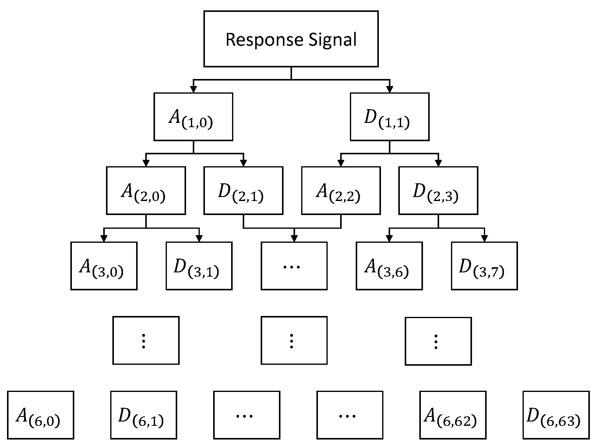
Time-domain features include common signal statistics: root mean square, variance, peak-to-peak, etc. Frequency domain features include root mean square of frequency, standard deviation of frequency and amplitude power spectrum, etc. The time–frequency joint feature is the statistical energy of different frequency bands obtained after six-layer wavelet packet decomposition, and its structure is shown in Figure 3.

Finally, each suspension system response signal has 75 statistical characteristic parameters, which can be found in the Appendix A.

3.

Feature reduction

The feature set generated in step 2 has a large amount of irrelevant and redundant information, which will degrade the performance of road classification models. In order to obtain the optimal feature combination quickly and accurately, this paper transforms the feature dimension reduction problem into a multi-objective optimization and selects the optimal features by the NSGA-II algorithm with the following parameters: a population size of 150, a number of generations of 200, and the probabilities of crossover and mutation are 0.9 and 0.1, respectively.

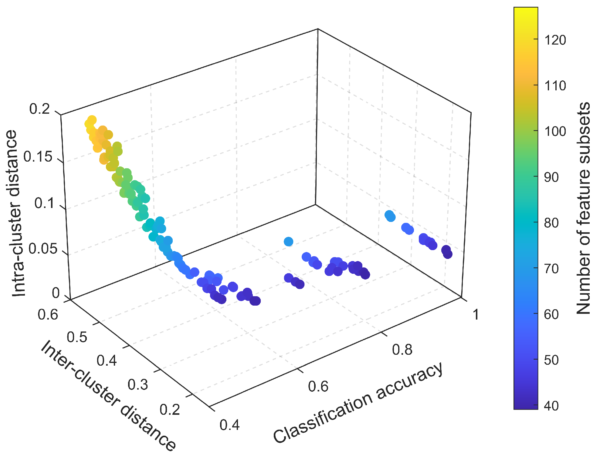
The Pareto optimal front, corresponding to the combination of optimal solutions that minimizes the classification model accuracy, the number of feature subsets, the feature inter-cluster distance and the intra-cluster distance, respectively, is shown in Figure 4.

Combining the importance of several evaluation metrics, the optimal subset of suspension characteristics includes the following 39 variables, which can be found in Appendix A.

4.

Classification:

The recognition accuracy of the road classification model needs to be used as an evaluation function for the NSGA-II algorithm; thus, in order to fully learn the suspension dynamic response feature, the receiver operating characteristic (ROC) curves are plotted in Figure 5 and the area under the ROC curve (AUC) values are calculated by testing the recognition results of different classification models. The classification models used for testing include Naive Bayes (NB), Narrow Bandwidth Neural Network (N-NN), K-Nearest Neighbor (KNN), Linear Support Vector Machine (L-SVM) and Decision Tree (DT), all of which are computed by the MATLAB Classification Learner toolbox. By selecting the L-SVM classification model with the highest AUC value, the unknown road level can be well determined.

Finally, when the unknown road level is determined by the classification algorithm, we can refer to the empirical nominal values corresponding to different roads given in

Table 1. Nominal values of Q and R for various ISO road levels.

Road Level	$\tilde{\mathit{Q}}$ Value	$\tilde{\mathit{R}}$ Value
		Sprung Mass	Unsprung Mass
A	0.0022	0.0001	0.0015
B	0.0088	0.0004	0.006
C	0.0351	0.0016	0.024
D	0.1406	0.0064	0.096
E	0.5624	0.0256	0.384
F	2.2495	0.1024	1.536
G	8.9979	0.4096	6.144
H	35.992	1.6384	24.576

[33].

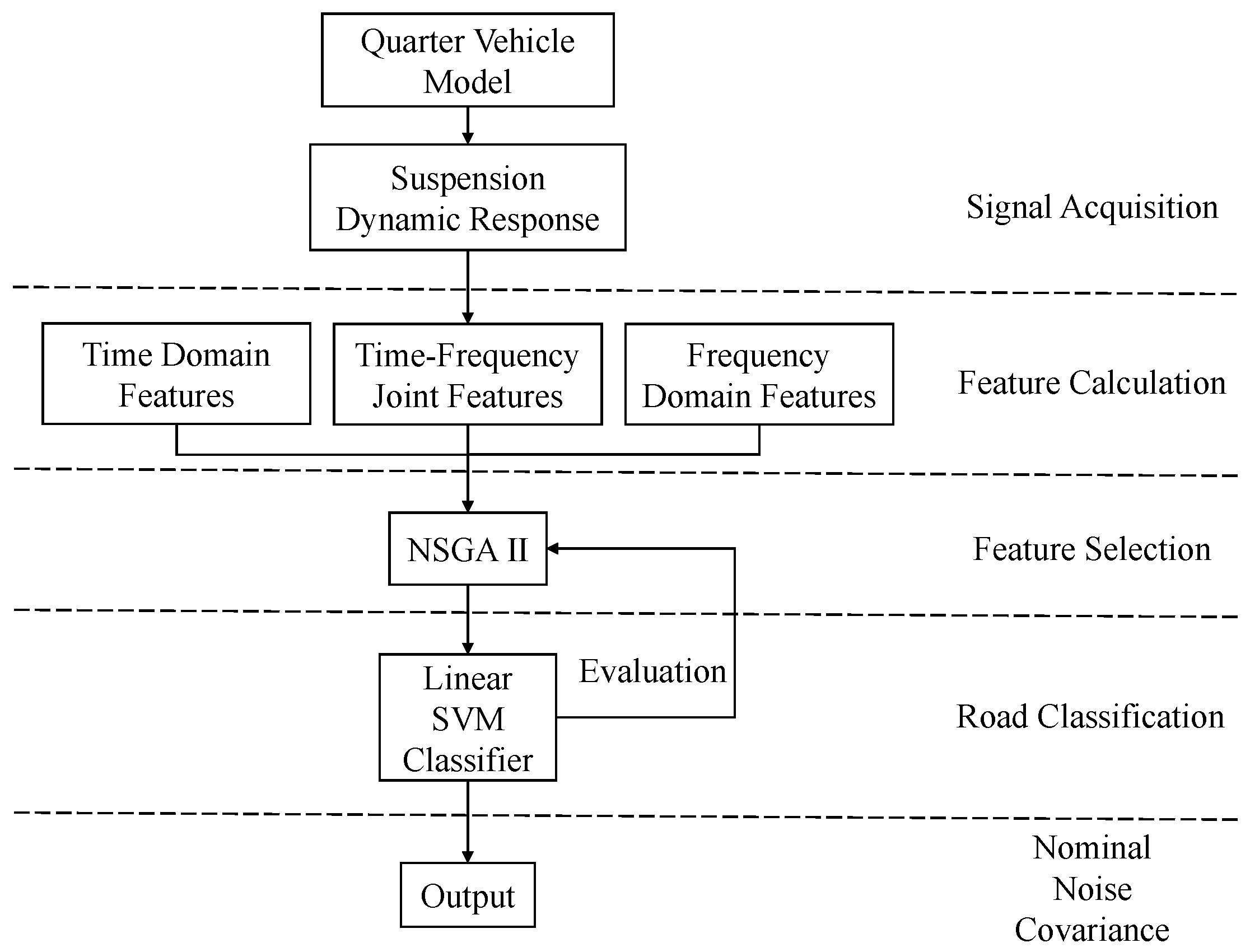
The above procedure of the proposed road classification scheme is summarized in Figure 6.

4. Simulations

The simulations in this paper focus on verifying the performance improvement effect of the proposed hybrid system based on VBAKF and road classification for 2-DOF suspension model state estimation with time-varying and unknown PNCM and MNCM. The source code is available at www.github.com/33lqq/Klaman. As mentioned in [34], the convergence principle of the Kalman filter is that the system parameters are in a time-invariant, detectable and stable state. Therefore, the suspension system considered in this paper only considers the linear time-varying system, and the 2-DOF suspension parameters are listed in

Table 2. Parameters for 2-DOF Suspension Model.

Suspension Parameters	Symbol and Unit	Value
Sprung mass	$m_s$-[kg]	250
Unsprung mass	$m_u$-[kg]	30
Suspension spring stiffness	$k_s$-[N/m]	10,000
Tyre stiffness	$k_t$-[N/m]	100,000
Suspension damping	$c_s$-[Ns/m]	1000

. The constant values of the system modeling parameters are chosen to ensure the convergence of the filter.

According to the random road surface modeling method described in [35,36], the time domain signal of a random road profile according to the ISO (International Organization for Standardization)-8608 standard can be expressed as

$$\begin{array}{c}\hfill z\left(t\right)=\sum _{i=1}^n\sqrt{2G_q\left(f_i\right)·\Delta f}sin(2\pi f_{i}t+{\theta }_i)\end{array}$$

(40)

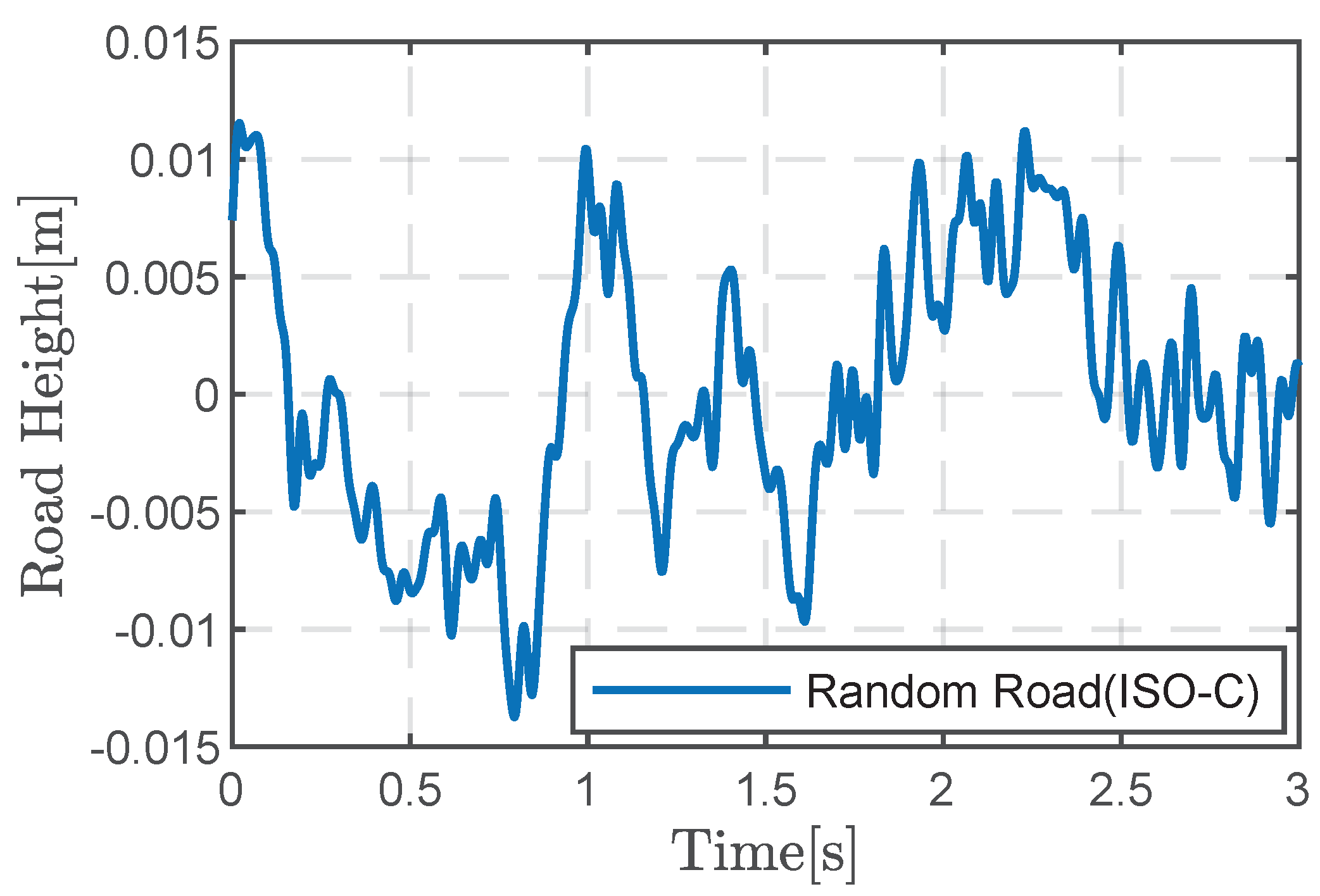
where n is the number of intervals obtained by uniformly dividing the frequency range of interest, center frequency $f_i$ and $\theta$ represents a random phase over $[0,2\pi ]$. Figure 7 shows the time domain spectrum of the ISO-C random road via Equation (40).

Considering that the state estimation error of the suspension system increases exponentially under different road levels, in this paper, in order to verify the robustness of the proposed state estimation algorithm, three different road sections are selected for simulation experiments, namely ISO-A, ISO-C and ISO-E.

The true values of the time-varying PNCM and MNCM can be assumed as follows:

$$\begin{array}{cc}\hfill Q_k& =\left(1-\cos \left(\frac{4\pi k}{T}\right)\right)\tilde{Q}\hfill \end{array}$$

(41)

$$\begin{array}{cc}\hfill R_k& =\left(1+\cos \left(\frac{4\pi k}{T}\right)\right)\tilde{R}\hfill \end{array}$$

(42)

where T = 1500 is the total number of discrete system simulations.

In addition, the initial parameters of the VBAKF algorithm in this paper are set as follows:

• The initial state $x_0$ and the error covariance matrix $P_0$ are assumed to be Gaussian distribution with $\mathrm{N}(0,1)$ for each component.
• Taking the nominal PNCM $\tilde{Q}$ and MNCM $\tilde{R}$ as the prior information of the IW distribution, the distribution parameter can be chosen as follows:

  $$\begin{array}{cc}\hfill t_0& =n_x+2,T_0=(t_0-n_x-1)\tilde{Q}\hfill \end{array}$$

  (43)

  $$\begin{array}{cc}\hfill u_0& =n_y+2,U_0=(u_0-n_y-1)\tilde{R}\hfill \end{array}$$

  (44)
• Finally, the forgetting factor is $\rho =1-\exp (-4)$, and the number of iterations is $N=10$.

Due to the different dimensions of the suspension state x, the root mean square error (RMSE) of the suspension state estimation cannot be calculated directly, so the simulation results are divided into two parts, namely the position component $x_1,x_2$ and the velocity component $x_3,x_4$. In addition, in order to eliminate the random errors caused by random numbers in the simulation process, we performed Monte Carlo (MC) operation, and used the average root mean square error (ARMSE) to quantitatively compare the performance of each filter on different road sections.

$$\begin{array}{cc}\hfill \mathrm{RMSE}\left(j\right)& \triangleq \left\{\begin{array}{cc}\sqrt{\frac{1}{M_c}{\sum }_{j=1}^{M_c}\left[{({\widehat{x}}_{1,k}^j-x_{1,k}^j)}^2+{({\widehat{x}}_{2,k}^j-x_{2,k}^j)}^2\right]},\hfill & \mathrm{position}\hfill \\ \sqrt{\frac{1}{M_c}{\sum }_{j=1}^{M_c}\left[{({\widehat{x}}_{3,k}^j-x_{3,k}^j)}^2+{({\widehat{x}}_{4,k}^j-x_{4,k}^j)}^2\right]},\hfill & \mathrm{velocity}.\hfill \end{array}\right.\hfill \end{array}$$

$$\begin{array}{cc}\hfill \mathrm{ARMSE}\left(j\right)& \triangleq \left\{\begin{array}{cc}\sqrt{\frac{1}{M_{c}T}{\sum }_{j=1}^{M_c}{\sum }_{k=1}^T\left[{({\widehat{x}}_{1,k}^j-x_{1,k}^j)}^2+{({\widehat{x}}_{2,k}^j-x_{2,k}^j)}^2\right]},\hfill & \mathrm{position}\hfill \\ \sqrt{\frac{1}{M_{c}T}{\sum }_{j=1}^{M_c}{\sum }_{k=1}^T\left[{({\widehat{x}}_{3,k}^j-x_{3,k}^j)}^2+{({\widehat{x}}_{4,k}^j-x_{4,k}^j)}^2\right]},\hfill & \mathrm{velocity}.\hfill \end{array}\right.\hfill \end{array}$$

where $M_c$ = 2000 represents the total number of the Monte Carlo runs, while ${\widehat{x}}_{i,k}^j$ and $x_{i,k}^j$ denote the estimated and true state of the ith component in the jth MC run.

The proposed hybrid systems are compared with the standard KF with true covariance matrices $Q_k$ and $R_k$ (KFTCM), the KF with nominal covariance ${\tilde{Q}}_k$ and ${\tilde{R}}_k$ (KFNCM), the AKF estimating $R_k$ based on the residual sequences (denoted by RSAKF) and the existing VBAKF estimating only $R_k$ (denoted by VBAKF-R).

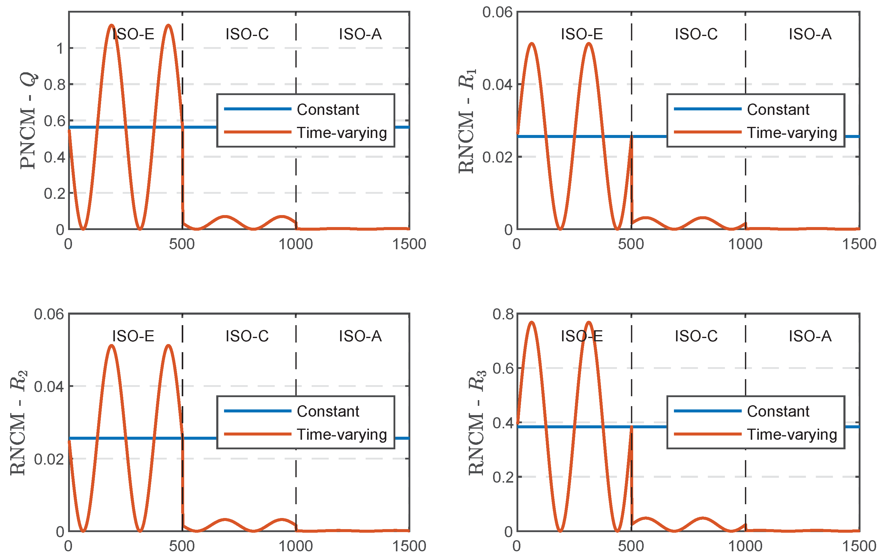
(1) First, we compare the performance results of different AKFs without road classification methods. Due to the lack of the guidance from the road classification model in the state estimation process, the suspension system cannot accurately identify the changes in the road profile level. Therefore, the nominal values of PNCM and MNCM throughout the entire simulation process only depend on the initial values of the road profile, as shown in Figure 8, where the nominal values on Stretch 2 (ISO-C) and Stretch 3 (ISO-A) have the same values as on Stretch 1 (ISO-E), i.e., the constant curve.

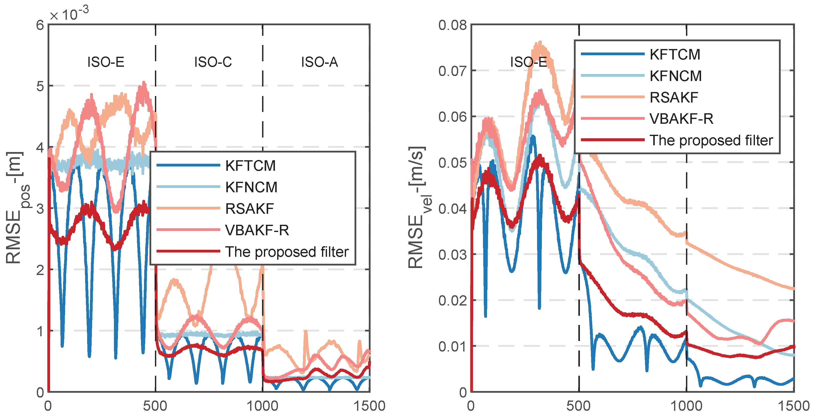
In Figure 9, from Stretch 1, it can be clearly seen that the proposed VBAKF filter algorithm is better than KFNCM, RSAKF and VBAKF-R. In

Table 3. The comparison of ARMSE in the position and velocity without road classification.

Filters	${\mathbf{ARMSE}}_{\mathbf{pos}}$
	Stretch1	Stretch2	Stretch3
KFTCM	0.0029	7.4761 $\times {10}^{-4}$	1.8678 $\times {10}^{-4}$
KFNCM	0.0037	9.4947 $\times {10}^{-4}$	2.3798 $\times {10}^{-4}$
RSAKF	0.0043	0.0018	6.4032 $\times {10}^{-4}$
VBAKF-R	0.0040	0.0010	4.3588 $\times {10}^{-4}$
The proposed filter	0.0027	6.8652 $\times {10}^{-4}$	2.7229 $\times {10}^{-4}$
Filters	${\mathrm{ARMSE}}_{\mathrm{vel}}$
KFTCM	0.0405	0.0124	0.0031
KFNCM	0.0511	0.0312	0.0129
RSAKF	0.0607	0.0414	0.0258
VBAKF-R	0.0561	0.0300	0.0129
The proposed filter	0.0430	0.0184	0.0086

, the ARMSEs of position and velocity from the proposed filter are respectively reduced by 27.03% and 15.85% compared to the existing KFNCM. In this section, the state estimation error of the proposed VBAKF filter algorithm is smoother than that of the KFTCM, and the maximum peak value is smaller than the latter. This is mainly due to the use of the Kalman smoother, which reduces the effect of time-varying fluctuations of the variance matrix on the state estimation process.

In Stretch 2 and Stretch 3, the state estimation errors of KFTCM, VBAKF-R and the VBAKF filter proposed in this paper are close to each other. This is because these two stretches use the incorrect PNCM and MNCM nominal values for state estimation, so these filters have difficulty converging to the true state in the limited iterative optimization.

Since RSAKF relies on the innovative sequence information of the historical sliding window, it is only applicable to the dynamic system for which the process noise matrix PNCM is known, so the continuous use of the incorrect PNCM nominal value leads to the continuous high level of state estimation error.

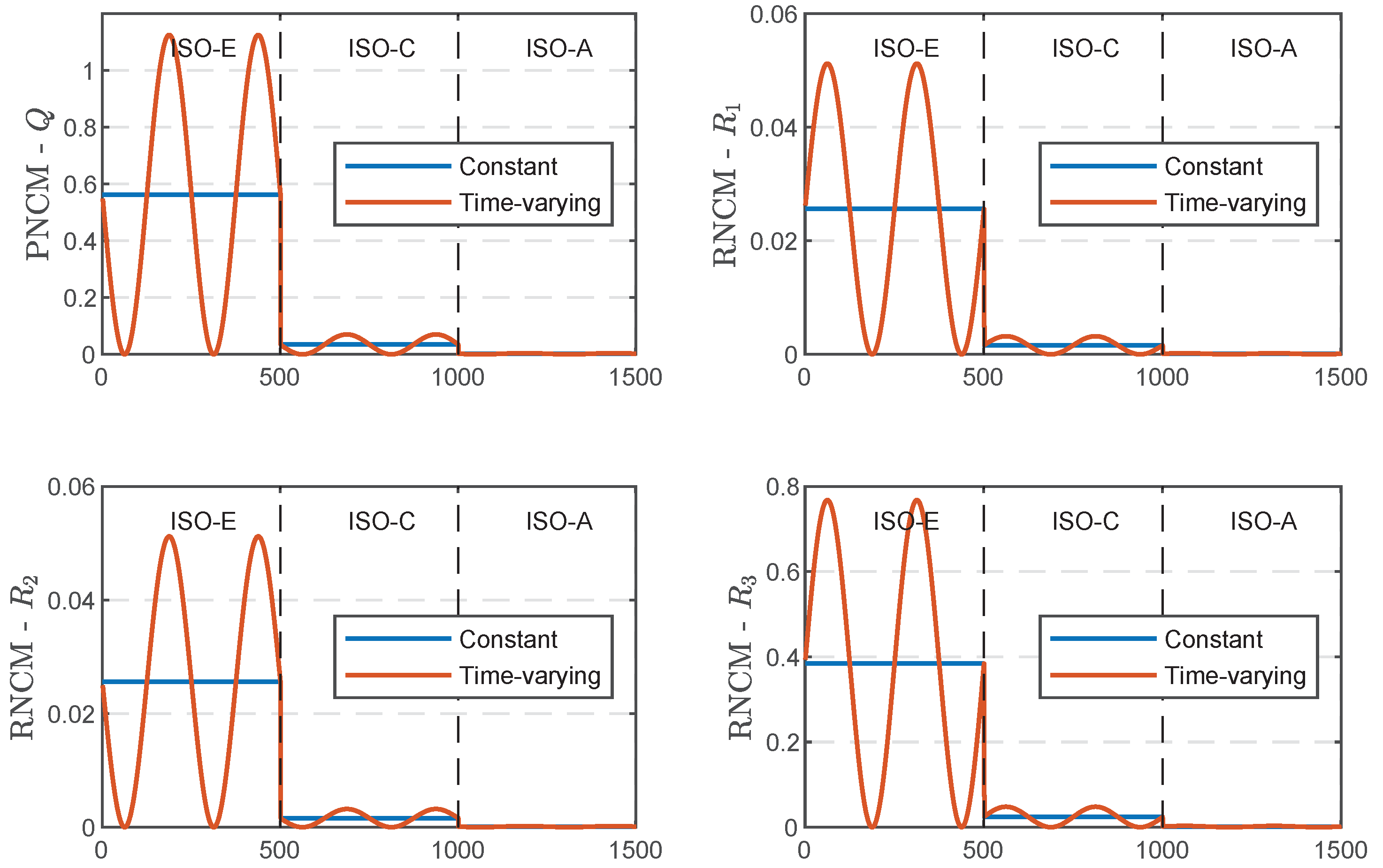
(2) Secondly, in order to verify the effectiveness of the road level classification algorithm for different adaptive filters, we still use three different random road profiles, as shown in Figure 10.

Unlike Figure 9, the nominal values of PNCM and MNCM corresponding to the current road level can be obtained by the road classification model.

In Figure 9, when the road profile level is unknown, the ARMSE of the position is only better than other filters only in segment 1. This segment is the initial road profile, and the nominal values of PNCM and MNCM have been given. In Figure 11, after using the road level classification algorithm, the road level of different segments can be accurately identified. In

Table 4. The comparisonof ARMSE in the position and velocity under road classification.

Filters	${\mathbf{ARMSE}}_{\mathbf{pos}}$
	Stretch1	Stretch2	Stretch3
KFTCM	0.0029	7.4727 $\times {10}^{-4}$	1.8688 $\times {10}^{-4}$
KFNCM	0.0037	9.4696 $\times {10}^{-4}$	2.3697 $\times {10}^{-4}$
RSAKF	0.0043	0.0011	2.7892 $\times {10}^{-4}$
VBAKF-R	0.0040	0.0010	2.5116 $\times {10}^{-4}$
The proposed filter	0.0027	6.7907 $\times {10}^{-4}$	1.7002 $\times {10}^{-4}$
Filters	${\mathrm{ARMSE}}_{\mathrm{vel}}$
KFTCM	0.0406	0.0125	0.0031
KFNCM	0.0512	0.0203	0.0053
RSAKF	0.0611	0.0240	0.0059
VBAKF-R	0.0559	0.0210	0.0054
The proposed filter	0.0398	0.0112	0.0038

, for each road segment, the proposed filters are better than other filters. For Stretch 2, the ARMSEs of position and velocity from the proposed filter are respectively reduced by 28.29% and 44.82% compared to the existing KFNCM. For Stretch 3, the proposed filter reduces the ARMSEs of position and velocity by 28.25% and 28.30%, respectively, compared to the existing KFNCM.

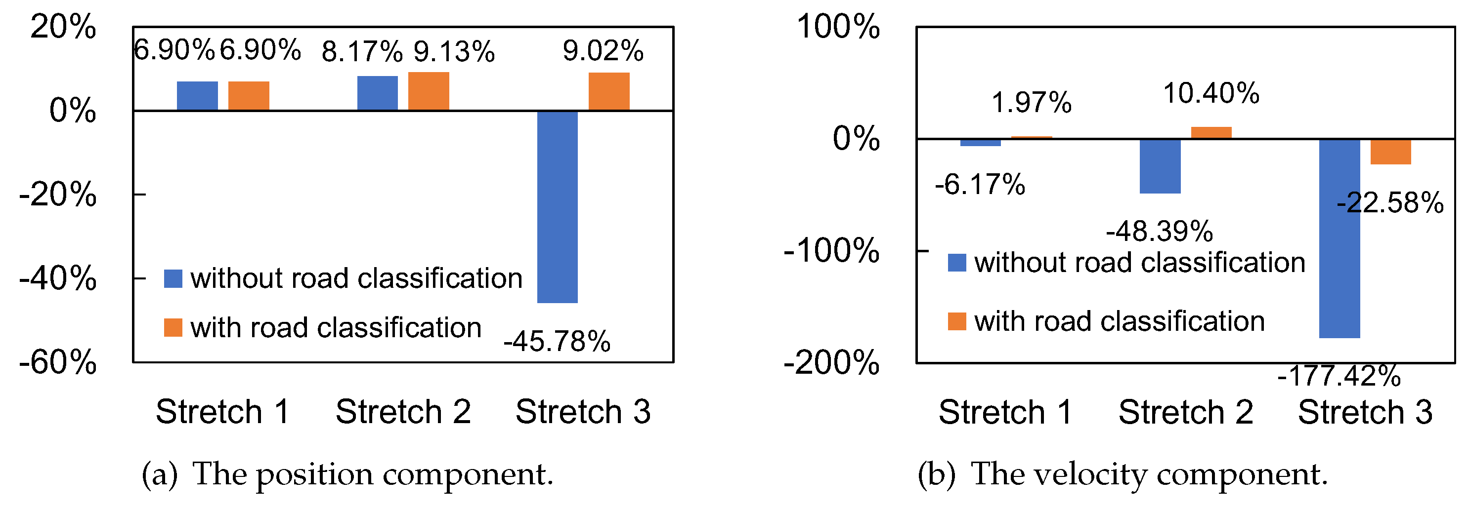
In Experiments 1 and 2, the AEMSEs of position and velocity of KFTCM remain essentially unchanged because the method uses the true values of PNCM and MNCM, while the presence or absence of road classification methods only affects the algorithms that depend on nominal values, i.e., KFNCM, RSAKF and VBAKF. Therefore, the performance improvement of the road classification method on the VBAKF algorithm can be evaluated by comparing the ARMSEs of the KFTCM and the filter proposed in this paper on the suspension state estimation in two experiments. As shown in Figure 12, the coordinates of the Y-axis coordinate represent the improvement rate of the proposed filter compared to KFTCM, and its calculation formula is as follows:

$$\frac{{\mathrm{ARMSE}}_{\mathrm{KFTCM}}-{\mathrm{ARMSE}}_{\mathrm{The}\mathrm{proposed}\mathrm{filter}}}{{\mathrm{ARMSE}}_{\mathrm{KFTCM}}}\times 100\%$$

Using the KFTCM as a benchmark for comparison, the use of the road category classification model significantly improved the state estimation accuracy of the VBAKF. In the second part, the performance of the location ARMS system was improved by 58.79% using the road surface identification method. In Section 3, the method improved the velocity ARMS and position ARMS by 57.8% and 154.84%, respectively. It can be noted that in Section 3, the accuracy improvement of the road classification algorithm for VBAKF estimation on ISO-A roads is exceptional. This improvement compared to ISO-C roads in Section 1 is mainly due to the low road variability in this region and the high accuracy of road class identification, which allows more accurate nominal values of the noise covariance matrix to be used during the state estimation iterations. In fact, this is not a performance improvement in the strict sense of the word. This improvement rate is calculated by the VBAKF algorithm relative to the road classification algorithm because the road classification model provides the filter with accurate PNCM and MNCM nominal values to avoid unknown nominal values causing the filter to converge in the wrong direction, i.e., increased state estimation error without VBAKF road classification.

In this experiment, the unknown characteristics of the road surface are transformed once at an interval of 500 sampling points. It is unlikely that the road surface category remains constant over time during the actual driving process, and the road surface class ahead of the vehicle is constantly changing. Of course, this type of problem can be solved by using sensors such as radar or cameras to obtain information about the road surface profile ahead and to identify the road surface class in advance. In addition, some specific road surface types such as concave and convex excitation, matrix excitation and triangular excitation are not considered in this paper and will be the focus of future studies.

5. Conclusions

In this paper, we develop a novel state estimation approach based on VBAKF and road classification to address the problem of suspension system state estimation with time-varying and unknown noise covariances. The main contributions of the paper are as follows:

(1)

The inverse Wishart distribution is used to approximate the time-varying covariance matrixes PECM and MNCM. Then, optimized state estimation is achieved by finite sampling the posterior PDF of the noise covariance and backward Kalman smoothing.

(2)

A road classification method with the input of the dynamic response of the suspension is proposed by combining multi-objective optimization and the linear classifier to accurately obtain the nominal values of PNCM and MNCM of the suspension system.

(3)

Compared with the existing filters, the developed novel state estimation approach makes an improvement in the estimation of the suspension state.