Data-Driven Nonlinear Iterative Inversion Suspension Control

Abstract

The commercial operation of the maglev train has strict requirements for the reliability and safety of the suspension control system. However, due to a large number of unmodeled dynamics of the suspension system, it is difficult to obtain the precise mathematical model of the suspension system. After the suspension system has been operated for a long time with high load, the system model will change due to the wear, aging and failure of components, as well as the settlement of the line and track. The control performance is degraded. Therefore, this paper proposes a data-driven nonlinear iterative inversion suspension control algorithm, which can achieve high-precision tracking performance recovery control after control performance degradation without depending on the suspension system model. The control performance of the suspension system is improved by learning the measured data of the historical suspension system, and the fast convergence of the tracking error and high-precision stable suspension control are realized in the presence of unmodeled dynamics and external noise interference. Based on the historical suspension data of the maglev train suspension control system, the inverse dynamics model of the suspension system is identified by iterative inversion learning based on data drive, and the suspension control framework based on iterative inversion is designed. Then, the nonlinear input update strategy is used to realize the rapid convergence of the learning process. Finally, the simulation experiment of the maglev train suspension system and the physical experiment of the maglev system experimental platform are combined. It is verified that the proposed levitation control algorithm can achieve high-precision fast tracking performance recovery control after the system control performance degrades under noise environment.

1. Introduction

As a new rail transit tool with mature technology, quiet operation, comfortable ride and high degree of localization, maglev train has become a popular means of transportation for citizens. Commercial operation lines, including Beijing Maglev Line S1, Changsha Maglev Express Line, Shanghai High speed Maglev Demonstration Line and Phoenix Culture Tourism Maglev Line, have been well integrated into people’s daily travel. In order to meet the strict requirements of the commercial operation reliability and operation performance of the maglev train, it is necessary to ensure that the suspension control system can always maintain a high performance working state. However, when the maglev train on the commercial operation line runs under a high load for a long time, the model parameters of the suspension system will change due to the wear, aging and failure of system components, as well as the track settlement of the line, which will lead to the deterioration of the control performance of the suspension control system. As the allowable variation range of the suspension gap is small, the maglev train will be prone to hit the track. This will affect the passenger’s riding experience. In serious cases, it may even affect the normal operation of the maglev train and endanger the safety of passengers. Therefore, in order to ensure the stable operation of the maglev train at the set suspension working gap of 10 mm, it is necessary to design a suspension control algorithm with high tracking performance.

The iterative learning control (ILC) method, which is used to implement repetitive control by learning from historical data to achieve high tracking performance, is widely popular for such problems as high-performance tracking control of suspension system clearance setting [1]. In this case, in order to improve the tracking performance of the suspension control, it is necessary to conduct accurate inverse dynamic modeling of the suspension system explicitly or implicitly. Accurate inverse dynamic model is very important to the performance of tracking control. The methods of constructing inverse models include model-based method and modeless method. Model-based iterative learning control uses the inverse model of the system as a learning filter for learning. If an accurate system model can be identified and the learning filter approximates the inverse dynamic model of the controlled object, the learning process can achieve rapid convergence [2,3]. Model-based methods usually use stable approximation [4,5] or numerical optimization [6,7] to obtain the inverse model.

However, model-based inversion of ILC requires sophisticated modeling, which is not practical in actual industrial sites. Zhongsheng Hou et al. also pointed out that due to the development of information science and technology, the complexity of industrial systems has increased, and it is difficult to model based on the first principle or identification method [8]. Therefore, it is very important to directly design controllers based on a large amount of data generated in industrial processes, which also promotes the development of data-driven control methods. Ronghu Chi et al. proposed a data-driven optimal terminal ILC method for linear and nonlinear discrete-time systems for fixed-input constant-value control systems [9,10]. The controller design only depends on the input and output measurement data of the system. Bolder et al. designed a data-driven steepest descent ILC method for the practical application of printing system control [11]. For these data-driven learning methods, the system model is constructed by model identification in the iterative learning process. Therefore, a modeless ILC method based on input-output data to identify the inverse dynamic model of the system is increasingly welcomed by researchers [12].

In addition, there are also ILCs based on compression mapping methods, such as D-type ILC, P-type ILC, PD-type ILC and PID-type ILC, and modeless methods based on time reversal ILC. The D-type ILC uses the derivative of the previous error signal to update the input, introducing high-frequency noise. Type P ILC avoids this problem. PD-type ILC can effectively ensure the convergence of tracking error. However, the tuning of PD parameters does not always meet the monotonic convergence conditions of the system, and the tuning process of PD parameters is particularly time consuming and may damage the system. Moreover, such methods based on contractive mapping require that the nonlinear terms of the system meet the global Lipschitz condition and have the same initial conditions. More significantly, such methods can only ensure that the system tracking error converges in the sense of the norm, and the weight of the norm is an exponential that decreases with time, so the tracking error will certainly decrease rapidly with time, which cannot accurately describe the dynamic characteristics of the system on the time axis. The transient problem caused by overshoot in the sense of a 2-norm cannot be avoided, and the fixed learning law form cannot adapt to the degradation of the system well. The ILC based on time reversal uses the adjoint operator of the system as the learning filter, and the iterative learning speed is slow.

Therefore, in order to achieve rapid error convergence, Kim et al. proposed a model free of iterative inversion-based control (MFIIC) method to estimate the inverse frequency response function (FRF) model based on the historical input and output data of the system [13]. It is unnecessary to determine the FRF model in advance, reducing the requirements for the model. However, when the system reference value is equivalent to the output interference, the performance will be significantly reduced. Pieter Janssens et al. proposed a data-driven constrained-norm optimal iterative learning control framework for linear time invariant systems for tracking and point to point motion problems [14]. They estimated the impulse response of the system using the input and output measurements of the previous iteration, eliminating time-consuming identification experiments.

The inverse dynamic model identification of the system can be obtained by solving the least squares problem in the time domain [15,16] or by point-by-point division in the frequency domain [17,18,19,20]. However, because there is no sustained excitation, these methods are usually sensitive to output disturbances, and the inverse model identification may not converge due to output disturbances. Therefore, ILC needs to balance the effective compensation of repetitive interference with the amplification effect of non-repetitive interference [21,22]. The key reason for ILC amplification of non-repetitive interference is that the effectiveness of repetitive interference is largely attributed to the non-causality in the time domain, while the essence of feedback control is causality, and ILC has strict causality in the iterative domain.

Since fast convergence can be obtained when the learning filter approaches the inverse system dynamics [23,24], a typical learning filter design method is based on the inversion of the parametric object model [3], which requires taking measures to ensure that the inverse of the non-minimum phase model is stable. The zero point of the non-minimum phase model means that the causal and stable inverse of the system does not exist, and the stable inverse is anti-causal [25]. For inverse causal inversion, the input required by the system can be determined according to the stable inversion process [26]. Because these methods are essentially model-based, requirements are put forward for parameter identification and approximate inversion of learning filters.

At present, although the system inverse dynamics estimation based on iterative learning reduces the requirement of prior modeling, the unmeasured interference of the system will still affect the convergence of iterative learning when the system inverse dynamics identification is conducted using historical test data.

Therefore, a data-driven nonlinear iterative inversion control method is designed in this paper to achieve high-precision fast-tracking suspension control of the maglev train so as to ensure that the suspension system of the maglev train can also ensure high-performance suspension tracking control when disturbed by track irregularities.

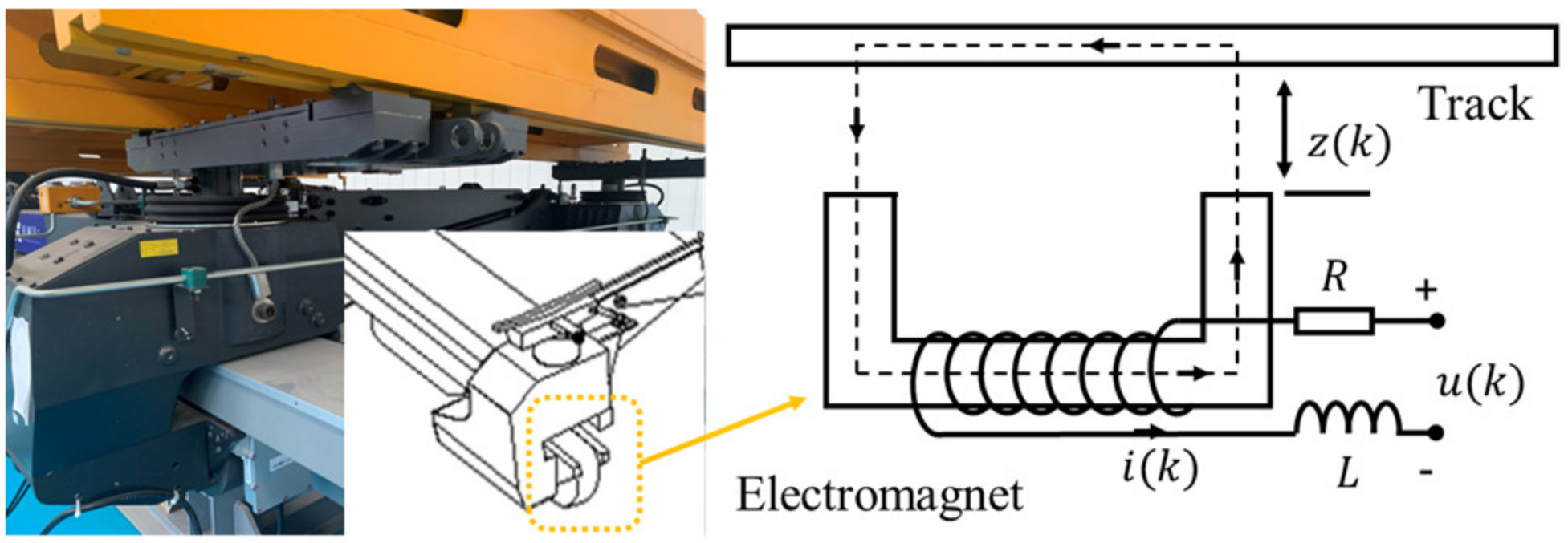
2. Maglev Control Problem Description

The main interference of the suspension control system is the track irregularity caused by the settlement of the maglev operation line track and the deformation of the track beam, which directly affects the measured value of the suspension gap. The vertical deflection of the track beam increases with the increase of the weight of the train and the span of the track beam. The track irregularity caused by the settlement of the line foundation or supporting pier will also affect the safe operation of the train. As shown in Figure 1. The lifting of the track outside the curve section of the maglev commercial operation line will also bring the influence of track irregularity to the maglev train suspension system. As shown in Figure 2.

In addition, for the control of maglev train suspension system, the following issues need to be considered:

(1)

The control input of the suspension system is limited (input saturation problem), mainly including the limitation of the output duty cycle of the suspension chopper and the limitation of the input current of the suspension controller. Working for a long time with an excessive current will cause the suspension electromagnet to overheat, which may affect the safe operation of the maglev train in serious cases.

(2)

The state of the maglev train suspension system is also limited. According to the structure of the suspension frame of the medium and low speed maglev train, the suspension gap in normal operation needs to be maintained at 8–12 mm.

(3)

Considering the actual operation of the maglev train, such as lifting, lowering, ramps and curves, the control of the suspension system needs to ensure passenger comfort on the maglev train during lifting and lowering, as well as the safe operation of the maglev train on ramps and curves under the influence of track irregularity.

(4)

Because the mileage of the maglev operation line is limited, the running time of the maglev train is limited, and the actual control performance of the maglev train cannot be guaranteed by the levitation control algorithm that requires the running time to reach infinity to obtain the gradual convergence effect.

(5)

The dynamic model of the actual suspension system of the maglev train has high-order nonlinear characteristics, and there are a lot of unmodeled dynamics, which makes it impossible to obtain an accurate model of the suspension system. At the same time, because the components of the suspension system will age or even fail, and the mechanical components will wear or even break after the maglev train runs for a long time, the model of the suspension system will also change. This means that the suspension control of the maglev train cannot simply rely on the accurate system model.

Therefore, aiming at the suspension control problem of maglev train suspension system in the presence of track irregularity interference, this paper makes full use of the characteristics of maglev train’s cyclic and repetitive operation and designs a data-driven nonlinear iterative inversion suspension control framework, as shown in Figure 3.

Where, $R$ is the reference value of the suspension gap, $E_i$ is the tracking error, $U_i$ is the control input of the suspension system, $D_i$ is the output interference of the suspension system, $Y_i$ is the output suspension gap, F is the learning filter, $F_i$ is the output signal of the i-th iteration of the learning filter, $G\left(z\right)$ is the z-domain form of the transfer function of the SISO discrete LTI suspension system that is gradually stable under zero initial conditions, and i is the number of iterations.

Assume that the time domain signal length of the system is infinite to meet the requirements of frequency domain analysis and avoid leakage in frequency domain calculation, that is $N\to \infty$. The entire impulse response is included in the object model [27].

$$G\left(z\right)\triangleq {\displaystyle \sum _{k=-N/2}^{N/2}g\left(k\right)z^{-k}}$$

(1)

where k is the time index of the discrete time signal, $g\left(k\right)\in ℝ$ is the impulse response of object $G$, and $u\left(k\right)\in ℝ$ and $y\left(k\right)\in ℝ$ are the input and output signals of the object respectively. Output signal $y\left(k\right)$ is obtained by convolving $g\left(k\right)$ and $u\left(k\right)$ in the time domain $y\left(k\right)=G\left(z\right)u\left(k\right)$. Therefore, the time domain update law of the general ILC algorithm is

$$u_{i+1}\left(k\right)=u_i\left(k\right)+F\left(z\right)\left[r\left(k\right)-y_i\left(k\right)\right]=u_i\left(k\right)+F\left(z\right)e_i\left(k\right),$$

(2)

where $r\left(k\right)$ is the reference signal of the system, $e_i\left(k\right)$ is the error signal of the i-th iteration of the system, and $u_i\left(k\right)$ and $y_i\left(k\right)$ are the input and output signals of the i-th iteration of the system respectively.

The general ILC algorithm will reset the initial condition $u_0\left(k\right)=F\left(z\right)r\left(k\right)$ before each iterative learning. Therefore, it can be obtained that the system tracking error is

$$\begin{array}{ccc}{e}_i\left(k\right)\hfill & =& r\left(k\right)-G\left(z\right)u_i\left(k\right)=r\left(k\right)-G\left(z\right)F\left(z\right){\displaystyle \sum _{n=0}^i{\left[1-G\left(z\right)F\left(z\right)\right]}^{n}r\left(k\right)}\\ & =& r\left(k\right){\left[1-G\left(z\right)F\left(z\right)\right]}^{i+1},\hfill \end{array}$$

(3)

Iterative tracking control needs to ensure that the tracking error converges to zero after multiple iterations. The goal is to minimize tracking error by updating feedforward using measurement data generated by previous control tasks. That is, for system $G\left(z\right)$, the ILC stability condition in frequency domain shown in Equation (4) needs to be satisfied.

$${\Vert I-G\left(z\right)F\left(z\right)\Vert }_{\infty }<1$$

(4)

where ${\Vert \cdot \Vert }_{\infty }$ denotes H∞-norm.

Therefore, the iterative tracking control problem needs to meet the following assumptions [27]:

Assumption 1. 

$R\left({\omega }_k\right)$ is the DFT form of the constant bounded reference input $R$, $Y_i\left({\omega }_k\right)$ is the DFT form of the output suspension gap, and the DFT form of the tracking error is

$$E_i\left({\omega }_k\right)\triangleq R\left({\omega }_k\right)-Y_i\left({\omega }_k\right)$$

(5)

where the output of the suspension system can be obtained by measurement, and its expression is

$$Y_i\left({\omega }_k\right)=G\left(e^{j{\omega }_k}\right)U_i\left({\omega }_k\right)+D_i\left({\omega }_k\right)$$

(6)

where $D_i\left({\omega }_k\right)$ is the DFT form of bounded track irregularity interference, and $\delta \left({\omega }_k\right)$ is the boundary, i.e., $\forall i$, so that

$$\left|D_i\left({\omega }_k\right)\right|\le \delta \left({\omega }_k\right)$$

(7)

This assumption is to achieve robustness to the worst-case estimation error. For the general ILC algorithm, the error signal is minimized by updating the feedforward with the measurement data from the previous task, thus improving the performance of repetitive control. For example, in the norm optimal ILC algorithm, suppose $r_{i+1}\left(k\right)=r_i\left(k\right)$ and the tracking error of the i-th iteration is [28]:

$$e_i\left(k\right)=S\left(z\right)r_i\left(k\right)-S\left(z\right)G\left(z\right)f_i\left(k\right)$$

(8)

where $S\left(z\right)={\left(I+G\left(z\right)C\left(z\right)\right)}^{-1}$ is the sensitivity function, and $f_i\left(k\right)$ is the output signal of the learning filter of the i-th iteration. The system minimizes the tracking error based on historical measurement data. Then the tracking error of the i + 1 iteration is

$$e_{i+1}\left(k\right)=e_i\left(k\right)+S\left(z\right)G\left(z\right)\left(f_i\left(k\right)-f_{i+1}\left(k\right)\right)$$

(9)

where the feedforward signal of the i + 1 iteration can be determined as

$$\begin{array}{ccc}{f}_{i+1}\left(k\right)\hfill & =& \underset{f_{i+1}}{\arg \min }V\left(f_{i+1}\left(k\right)\right)\hfill \\ & =& \underset{f_{i+1}}{\arg \min }(\Vert e_{i+1}\left(f_{i+1}\left(k\right)\right)\Vert W_e+\Vert f_{i+1}\left(k\right)\Vert W_f+\Vert f_{i+1}\left(k\right)-f_i\left(k\right)\Vert W_{\Delta f}),\hfill \end{array}$$

(10)

$V\left(f_{i+1}\left(k\right)\right)$ is a data-based performance standard, $W_e>0$ is a positive definite weight matrix, and $W_f\ge 0$ and $W_{\Delta f}\ge 0$ are semi positive definite weight matrices, which are used to balance the robustness and convergence of iterative learning algorithms. However, due to the influence of track irregularity, the reference signal $r\left(k\right)$ of the suspension control system will change, making the key assumptions of the ILC algorithm no longer meet, which will lead to the decline of the tracking performance of the ILC algorithm.

3. Model Free Nonlinear Iterative Inverse Learning Control for Suspension System

Considering the existence of track irregularity in levitation control, a data-driven iterative inversion learning control update law is determined as [29]

$$U_{i+1}\left({\omega }_k\right)=f\left(U_i\left({\omega }_k\right),Y_i\left({\omega }_k\right),R\left({\omega }_k\right)\right)$$

(11)

$$f\left(U_i,Y_i,R\right)=\{\begin{array}{l}{U}_i+\rho \left(\left|Y_i\right|\right)\frac{U_i}{Y_i}{E}_i,Y_i\ne 0,\\ U_i,Y_i=0,\end{array}$$

(12)

where $\rho \in ℝ$ is the gain learning function, $\rho \ge 0$ and $i\ge 1$. The basic principle is to use $\rho \left(\left|Y_i\right|\right)$ to avoid unbounded amplification of input.

In addition, if the system is disturbed by changes, the tracking error will not converge to 0. Define the tracking error change rate as

$$\Delta \delta \left({\omega }_k\right)\triangleq \underset{i\ge 0}{\max }\left|D_i\left({\omega }_k\right)-D_{i+1}\left({\omega }_k\right)\right|$$

(13)

3.1. Tracking Performance Conditions Based on Nonlinear IIL

Consider the update law given in Equation (12). If for $\alpha >1$, the following constraints are satisfied [29]:

$$\left(\alpha -1\right)/\alpha \le \rho \left(\left|Y_i\right|\right)\le 1$$

(14)

$$\left|R\right|\ge \alpha \delta +\Delta \delta \alpha /\left(\alpha -1\right)$$

(15)

$$\left|E_0\right|\le \left|R\right|-\alpha \delta ,$$

(16)

where $E_0$ is the initial tracking error. Then we can obtain

$$\underset{i\to \infty }{\lim }{E}_i\in \left\{x\in ℂ|\left|x-z\right|\le r,z=0,r=\Delta \delta \frac{\alpha }{\alpha -1}\right\}$$

(17)

When $\Delta \delta =0$ and sequence $\left\{E_i\right\}$ converge monotonically to $E_{\infty }=0$. Therefore, when the following conditions are met, the error asymptotic convergence can be guaranteed: (1) The learning gain $\rho \left(\left|Y_i\right|\right)$ has a non-zero strict lower bound, which does not exceed 1; (2) $\left|R\right|$ is much larger than $\delta$ and $\Delta \delta$; (3) The initial tracking error is far less than $\left|R\right|$ and $\delta$; and (4) The tracking error converges to the neighborhood of 0, which is proportional to $\Delta \delta$. This conclusion can be proved by the following lemma [29]:

Lemma 1. 

Each sequence ${\left\{E_i\right\}}_{i=0}^{\infty }$ satisfies the following boundary conditions,

$$\left|E_{i+1}\right|\le k_i\left|E_i\right|+\Delta \delta ,i\ge 0$$

(18)

$$\left|E_i\right|\le {\overline{k}}^i\left|E_0\right|+\Delta \delta \left({\overline{k}}^i-1\right)/\left(\overline{k}-1\right),i\ge 0$$

(19)

$$k_i\triangleq \left|\left(\left(1-\rho \left(\left|Y_i\right|\right)\right)\left(R-E_i\right)+\rho \left(\left|Y_i\right|\right)D_i\right)/\left(R-E_i\right)\right|$$

(20)

where $\overline{k}\in ℝ,\overline{k}\ge 0$ and $\forall i$ satisfies $k_i\le \overline{k}$.

Lemma 2. 

If there is $\left(\alpha -1\right)/\alpha <\rho \left(\left|Y_i\right|\right)\le 1,\left|R\right|\ge \alpha \delta$ for $\alpha >1$, and

$$\left|E_i\right|\le \left|R\right|-\alpha \delta$$

(21)

then $k_i\le 1/\alpha$, where $k_i$ is given by Equation (20).

3.2. Convergence Analysis

For $\alpha <1$, given Equations (14)–(16), $\forall i$ makes Equation (21) hold. It needs to be proven that if Equation (21) holds for i, then Equation (21) holds for i + 1.

In order to obtain this conclusion, suppose that Equation (21) is true for i, according to Lemma 2, $k_i\le 1/\alpha$, combined with Equation (15) $\left|R\right|\ge \alpha \delta +\Delta \delta /\left(1-k_i\right)$, we can obtain $k_i\left(\left|R\right|-\alpha \delta \right)+\Delta \delta \le \left|R\right|-\alpha \delta$, and because Equation (21) is true for i, we can obtain $k_i\left|E_i\right|+\Delta \delta \le \left|R\right|-\alpha \delta$, and then we can obtain $\left|E_{i+1}\right|\le \left|R\right|-\alpha \delta$ according to Equation (18).

Therefore, if Equation (21) is true for i, then it is also true for i + 1. Since Equation (21) is also true when i = 0, it is proven that Equation (21) is true for $\forall i$ [29].

According to Lemma 2, $\forall i$ makes $k_i\le 1/\alpha <1$. Therefore, for $i\to \infty$,

$$\underset{i\to \infty }{\lim }\left|E_i\left({\omega }_k\right)\right|\le \Delta \delta \alpha /\left(\alpha -1\right)$$

(22)

This also proves Equation (17). In addition, if $\Delta \delta =0$, we can directly draw the conclusion that ${\left\{E_i\right\}}_{i=0}^{\infty }$ converges monotonically to 0 from Equation (18) in Lemma 1.

In addition, for the iterative inversion learning control update law of Equation (18), the input can converge to the neighborhood of the limit point.

According to the following Theorem 1, if the error converges to the neighborhood of 0, the input will converge to the neighborhood of $U_{\infty }$ [29]:

Theorem 1. 

Consider Equation (12) under the condition of Assumption 1. If Equations (14)–(16) hold for $\alpha >1$ then

$$\{\begin{array}{l}\underset{i\to \infty }{\lim }{U}_i\in \{x\in ℂ|\left|x-U_{\infty }\right|\le r,U_{\infty }=G^{-1}R,\\ r=\left|G^{-1}\right|(\Delta \delta \alpha /\left(\alpha -1\right)+\delta )\},\end{array}$$

(23)

for the case of $\Delta \delta =0$, ${\left\{U_i\right\}}_{i=0}^{\infty }$ converges to $U_{\infty }=G^{-1}\left(R-D\right)$.

In addition, when the reference is relatively small relative to the interference, Theorem 2 can be obtained [29].

Theorem 2. 

Under the condition of Assumption 1, consider Equation (12), if $0<\rho \left(\left|Y_i\right|\right)\le 1$, $\left|Y_i\right|\ne 0$, for $\beta >1$, then $\forall i$ makes reference $\beta \left|R\right|\le \left|D_i\right|$, and the initial input is

$$\left|U_0\right|<\left(\beta -1\right)\left|G^{-1}R\right|$$

(24)

then sequence ${\left\{U_i\right\}}_{i=0}^{\infty }$ of Equation (12) converges monotonically to $U_{\infty }=0$.

According to Theorem 2, if $\left|R\right|$ is smaller than $\left|D_i\right|$, then $U_i$ will converge to 0. This is obviously different from the iterative learning method based on the update law of the inverse model. In this method, if the convergence condition is not satisfied, the unstable iterative dynamics may lead to unbounded input. However, in NLIIC, the iterative update will not result in unbounded input, and the input will converge to 0. Theorem 2 can be proven by Lemmas 3 and 4 [29]:

Lemma 3. 

Under the condition of Assumption 1, consider Equation (12), and each sequence ${\left\{U_i\right\}}_{i=0}^{\infty }$ satisfies

$$U_{i+1}=\left(\frac{\left(1-\rho \left(\left|Y_i\right|\right)\right)\left(G{U}_i+D_i\right)+\rho \left(\left|Y_i\right|\right)R}{G{U}_i+D_i}\right)U_i$$

(25)

 that is, each sequence ${\left\{U_i\right\}}_{i=0}^{\infty }$ meets the following restrictions

$$\left|U_{i+1}\right|=k_i\left|U_i\right|,i\ge 0$$

(26)

$$k_i\triangleq \left|\frac{\left(1-\rho \left(\left|Y_i\right|\right)\right)\left(G{U}_i+D_i\right)+\rho \left(\left|Y_i\right|\right)R}{G{U}_i+D_i}\right|$$

(27)

where $\forall i$, $\overline{k}\in ℝ$ and $\overline{k}\ge 0$, meet $k_i\le \overline{k}$.

Lemma 4. 

If $0<\rho \left(\left|Y_i\right|\right)\le 1$, for $Y\ne 0$ and $\beta >1$, $\forall i$ makes $\beta \left|R\right|\le \left|D_i\right|$ true, and $\forall i$, makes $\left|U_i\right|<\left(\beta -1\right)\left|G^{-1}R\right|$ true.

The proof of Theorem 2 is as follows: Given $0<\rho \left(\left|Y_i\right|\right)\le 1$ for $Y_i\ne 0$ and for $\beta >1$, $\forall i$ let $\beta \left|R\right|\le \left|D_i\right|$ and $\left|U_0\right|<\left(\beta -1\right)\left|G^{-1}R\right|$ hold according to Lemma 4. For A, it is equivalent to B. Because of C, according to D, E can be obtained. Then according to Lemma 4, we can know $k_1<1$. Repeat the above process to obtain $\forall i$, $k_i<1$. Therefore, Theorem 2 proves thatTherefore, Theorem 2 proves that ${\left\{U_i\right\}}_{i=0}^{\infty }$ converges to $U_{\infty }=0$.

This section mainly analyzes the system input convergence of the control algorithm. In addition, according to the reference [20], the conditions that need to be satisfied to obtain the bounded input amplification $\rho \left(\left|Y_i\right|\right)$ can be derived, so as to ensure the global input convergence of the system. According to Equation (27),

$$\begin{array}{ccc}{k}_i\hfill & \le & \left(\left|Y_i\right|+\rho \left(\left|Y_i\right|\right)\left|Y_i\right|+\rho \left(\left|Y_i\right|\right)\left|R\right|\right)/\left|Y_i\right|\hfill \\ & \le & 1+\rho \left(\left|Y_i\right|\right)+\left|R\right|\left|\rho \left(\left|Y_i\right|\right)\right|/\left|Y_i\right|\hfill \\ & \le & 1+\overline{\rho }+\left|R\right|\tau ,\hfill \end{array}$$

(28)

where $\tau \triangleq \underset{\left|Y_i\right|\ne 0}{\sup }\left(\rho \left|Y_i\right|/\left|Y_i\right|\right)$ and $\overline{\rho }\triangleq \underset{\left|Y_i\right|\ne 0}{\sup }\left(\rho \left|Y_i\right|\right)$.

Therefore, $\forall x\in \left(0,\infty \right)$, if and only if $f\left(x\right)\triangleq \rho \left(x\right)/x$ is bounded, the third term on the right side of Equation (28) is bounded. Under the assumption of 1, if $\rho \left(x\right)$ is continuous in the neighborhood of 0, and $\underset{x\to 0}{\lim }\rho \left(x\right)=0$ and $\left(d\rho /d\left|Y_i\right|\right){|}_{\left|Y_i\right|=0}\in ℝ$ exist, then $\forall x\in \left(0,\infty \right)$, the real function $f\left(x\right)\triangleq \rho \left(x\right)/x$ is bounded, and $\left|R\right|$ is bounded.

Therefore, under the assumption of 1, if $\rho \left(\left|Y_i\right|\right)$ is continuous in the neighborhood of 0, $\underset{\left|Y_i\right|\to 0}{\lim }\rho \left(\left|Y_i\right|\right)=0$, and $\left(d\rho /d\left|Y_i\right|\right){|}_{\left|Y_i\right|=0}\in ℝ$ exists, then $\forall i$, $\left|U_{i+1}\right|\le \overline{k}\left|U_i\right|$,

$$\overline{k}=1+\overline{\rho }+\tau \left|R\right|$$

(29)

This conclusion shows that if $\rho \left(\left|Y_i\right|\right)$ is continuous near 0, when $\left|Y\right|\to 0$, $\rho \left(\left|Y_i\right|\right)\to 0$, and $\rho \left(\left|Y_i\right|\right)$ is differentiable near 0, then $\overline{k}$ satisfies an upper bound. Therefore, for the iterative inverse learning control update law designed in this paper, the amplification of the system input is bounded. This conclusion also provides a global guarantee for the convergence of the system input [29].

In this section, the input amplification is adjusted by using the learning gain function $\rho \left(\left|Y_i\right|\right)$. If $\rho \left(\left|Y_i\right|\right)$ and $\left|R\right|$ meet specific attributes, NLIIC can solve the problem of data-driven iterative tracking.

In the next section, we will study the limitations of traditional MFIIC to help design specific gain functions, so as to design and complete the data-driven iterative inversion levitation control algorithm.

3.3. Data-Driven Nonlinear Iterative Inversion Suspension Control Algorithm

In this section, the IIC algorithm and the limitations of MFIIC algorithm are reviewed to help design a data-driven nonlinear iterative inversion levitation control algorithm.

According to the literature [13], when the modeling error is not too large and the iterative coefficient is selected, IIC algorithm can achieve accurate tracking, but the algorithm is sensitive to the phase uncertainty of system dynamics, especially when the phase uncertainty is close to $\pi /2$.

MFIIC updates the inverse model by using input and output measurement data in each iteration, and makes the iteration coefficient 1, which not only eliminates IIC’s modeling process and its related model quality and modeling time consuming problems but also improves the quality of the inverse model through iteration [13]. Considering the case of NLIIC $\rho \left(\left|Y_i\right|\right)=1$, NLIIC will be simplified to the traditional MFIIC. Obviously, when $Y_i\to 0$, $\underset{\left|Y_i\right|\to 0}{\lim }{k}_i=\infty$, the boundedness of input amplification cannot be guaranteed. According to MFIIC [30],

$$U_i=\frac{GR}{G\left(1+S_i\right)+P_i/\alpha },\forall i\ge 1$$

(30)

$$P_i={\displaystyle \prod _{j=0}^{i-1}{D}_j/R},S_i=\{\begin{array}{l}0,i=1,\\ {\displaystyle \sum _{n=1}^{i-1}{\displaystyle \prod _{j=1}^n{D}_{i-j}/R}},i\ge 2,\end{array}$$

(31)

For random noise and non-random effects (such as nonlinear dynamics not modeled), as long as $D_i/R$ is small enough, the iterative process will make the noise correlation terms $P_i$ and $S_i$ tend to zero. For $\forall i$, when $\exists \epsilon$ makes $\left|D_i/R\right|\le \epsilon <0.5$, the relative tracking error is bounded,

$$\underset{i\to \infty }{\lim }\left|\left(Y_i-R\right)/R\right|\le 2\epsilon \left(1-\epsilon \right)/\left(1-2\epsilon \right)$$

(32)

when $\epsilon <1-\sqrt{2}/2\approx 0.3$, $\underset{i\to \infty }{\lim }\left|\left(Y_i-R\right)/R\right|<1$. This ensures MFIIC’s ability to improve output tracking. Therefore, MFIIC can improve the tracking performance and input convergence performance of the system. Therefore, the gain function designed in this section is [29]

$$\rho \left|Y_i\right|=\{\begin{array}{l}1,\left|Y_i\right|>\gamma ,\\ 0.5\left(1-\cos \left(\pi \left|Y_i\right|/\gamma \right)\right),\left|Y_i\right|\le \gamma ,\end{array}$$

(33)

when $\gamma >0$, $\left|Y_i\right|>\gamma$, $\rho \left|Y_i\right|=1$, and $\gamma =\left|R\right|$ are often used. Therefore, when $\left|R\right|>\delta$ and $k_i=\left|D_i\right|/\left|Y_i\right|\le \delta /\left|Y_i\right|\le \left|R\right|/\left|Y_i\right|<1$, MFIIC is used for reference, the tracking performance of the system increases monotonously, and the system input is strictly reduced during iteration.

When $\left|Y_i\right|\le \gamma$ is selected, NLIIC is used for reference to ensure that the amplification of system input is bounded.

$$\{\begin{array}{l}\underset{\left|Y_i\right|\to 0}{\lim }{k}_i\le 1+\rho \left(\left|Y_0\right|\right)+\left|R\right|\underset{\left|Y_i\right|\to 0}{\lim }\left(\rho \left(\left|Y_i\right|\right)/\left|Y_i\right|\right)=1,\\ \overline{k}=1+\overline{\rho }+\tau \left|R\right|\le 2+\tau \left|R\right|,\end{array}$$

(34)

$$\begin{array}{c}\frac{d}{d\left|Y_i\right|}\left(\frac{\rho \left|Y_i\right|}{\left|Y_i\right|}\right)=\frac{d}{d\left|Y_i\right|}\left(\frac{1-\cos \left(\pi \left|Y_i\right|/\gamma \right)}{2\left|Y_i\right|}\right)=\frac{2\left|Y_i\right|\frac{\pi }{\gamma }\sin \left(\pi \left|Y_i\right|/\gamma \right)-2\left(1-\cos \left(\pi \left|Y_i\right|/\gamma \right)\right)}{4{\left|Y_i\right|}^2}\\ \hspace{1em}\hspace{1em}\hspace{1em}\hspace{1em} =\mu \sin \left(\mu \right)-1+\cos \left(\mu \right),\end{array}$$

(35)

where $\mu \in \left(0,\pi \right]$, when $\mu \approx 2.33$,

$$\tau =\underset{\left|Y_i\right|>0}{\sup }\left(\rho \left|Y_i\right|/\left|Y_i\right|\right)=\left(1-\cos \left(\mu \right)\right)\pi /\left(2\gamma \mu \right)$$

(36)

Therefore, the input is bounded.

In addition, in order to improve the robustness of the control system, especially considering the influence of high-frequency model uncertainty and to achieve a low tracking error in the steady state of the system, the adjoint-based learning method is used for reference. Design the initial switching learning filter $F_0\left(z\right)=\alpha G^{*}\left(z\right)$, and make the gain $\alpha >0$ small enough to ensure the stability condition,

$${\Vert 1-F_0\left(z\right)G\left(z\right)\Vert }_{\infty }<1$$

(37)

Among them, $\alpha G^{*}\left(z\right)e_i\left(k\right)$ can be obtained based on modeless time inversion filtering technology [28], as shown in Algorithm 1.

Algorithm 1: Calculating ILC learning law based on time inversion
S1	Reverse the error signal $e{1}_i\left(k\right)=e_i\left(N-k\right)$.
S2	Apply the reverse error signal $e{1}_i\left(k\right)$ to the system to obtain the output signal:$e{2}_i\left(k\right)=G\left(z\right)e{1}_i\left(k\right)$.
S3	Then reverse the output signal and multiply by a factor small enough:$e{3}_i\left(k\right)=\alpha e{2}_i\left(N-k\right)$.
S4	Finally, the learning law based on adjoint is:$u_{i+1}\left(k\right)=u_i\left(k\right)+\alpha G^{*}\left(z\right)e_i\left(k\right)=u_i\left(k\right)+e{3}_i\left(k\right)$.

However, a small gain $\alpha$ will result in slow convergence. Therefore, this paper combines the advantages of MFIIC’s fast convergence, low steady-state tracking error based on time inversion filtering, and the advantages of NLIIC’s high tracking performance in the presence of interference and designs a data-driven nonlinear iterative inversion levitation control algorithm. The computational cost of the algorithm inherits the advantages of MFIIC. Its time complexity is $\mathbf{O}(n)$ and space complexity is $\mathbf{O}(1)$. Therefore, the iterative learning speed of the algorithm is fast, as shown in Figure 4. The algorithm flow is shown in Algorithm 2.

Algorithm 2: Data-driven nonlinear iterative inversion learning control based on time inversion
S1	Initialize, select system initial input: $u_0\left(k\right)=r\left(k\right)$, $F_0\left(z\right)=\alpha G^{*}\left(z\right)$.
S2	Apply input $u_i\left(k\right)$ to the system to obtain output $y_i\left(k\right)$, and then calculate the tracking error $e_i\left(k\right)=r\left(k\right)-y_i\left(k\right)$ of the system. If the tracking error is small enough and within the acceptable range, stop the iterative learning process or go to the next step.
S3	If $i=0$, go to step 4, otherwise go to step 5.
S4	Execute the ILC based on time inversion, $u_{i+1}\left(k\right)=u_i\left(k\right)+\alpha G^{*}\left(z\right)e_i\left(k\right)$, and then let $i=i+1$. Go to step 2 for execution.
S5	Discrete Fourier transform is used to obtain frequency domain signals $U_i\left({\omega }_k\right)$ and $E_i\left({\omega }_k\right)$.
S6	Then combine learning gain function $\rho \left(\left|Y_i\right|\right)$ and obtain $U_{i+1}\left({\omega }_k\right)$ according to Equation (11). Finally, perform IDFT to obtain time domain $u_{i+1}\left(k\right)$, and then turn to step 2 for $i=i+1$ to execute.

In the iterative learning process, the inverse model is applied to the learning filter of the nonlinear iterative inversion levitation control algorithm to accelerate the convergence of the tracking error [27,31]. The learning filter update structure is shown in Figure 5. Once the tracking error converges, the inverse model-based optimal learning filter can be used to track any trajectory. The learning filter update algorithm flow based on the inverse model is shown in Algorithm 3.

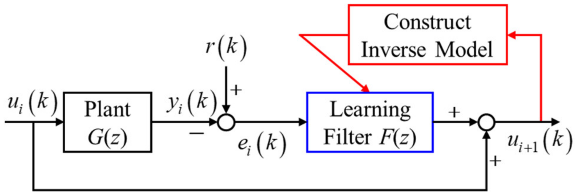
Algorithm 3: Update learning filter
S1	Initialize the reference pulse signal to $r\left(k\right)=\alpha \delta \left(k\right)$. Execute the algorithm initialization in Algorithm 2.
S2	Perform the algorithm iteration update steps in Algorithm 2.
S3	Construct the inverse model as $\overline{G}\left(z\right)={\displaystyle {\sum }_{k=-N/2}^{N/2}u\left(k\right)z^{-k}}$.
S4	Finally, the updated learning filter is replaced by the inverse model.

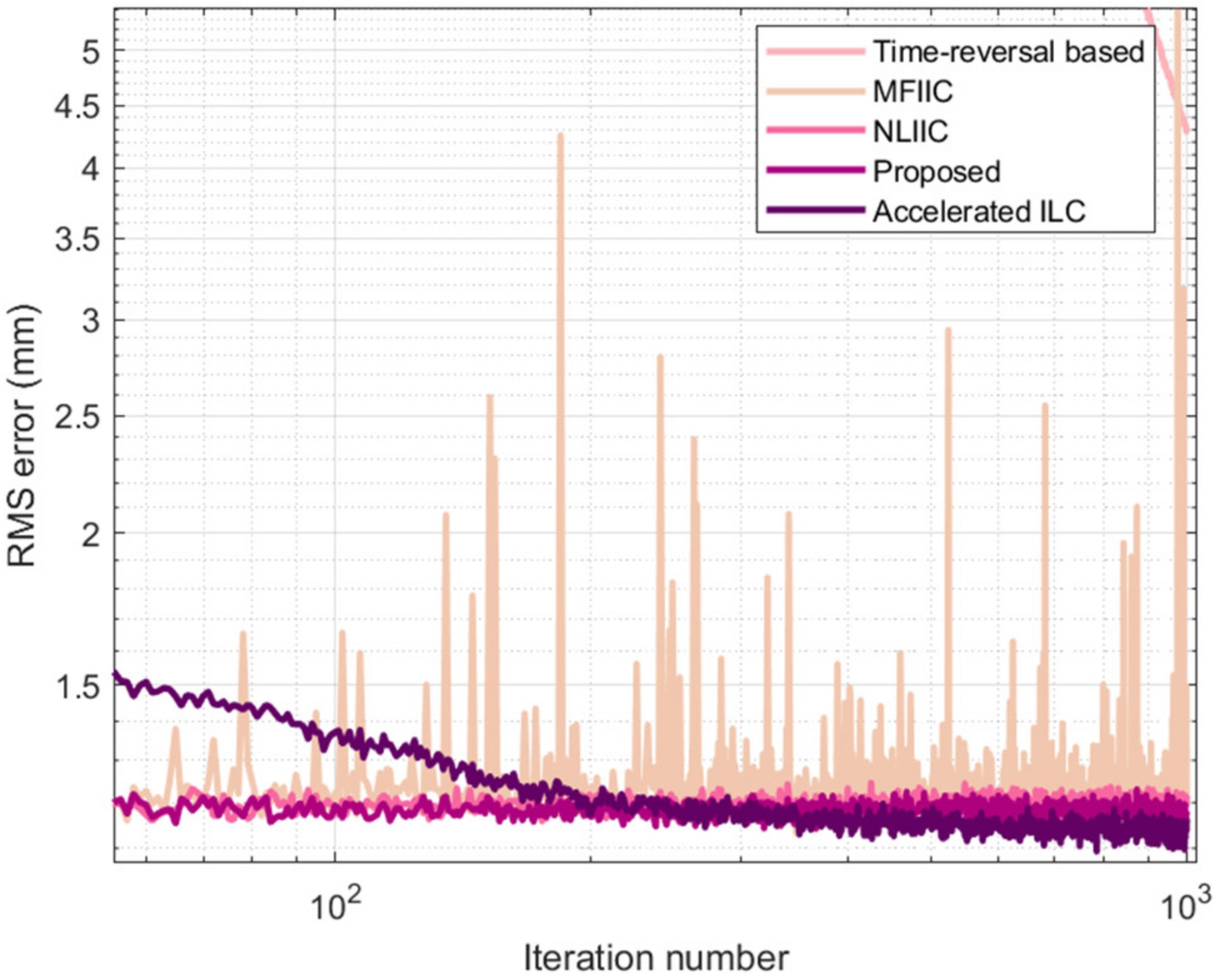
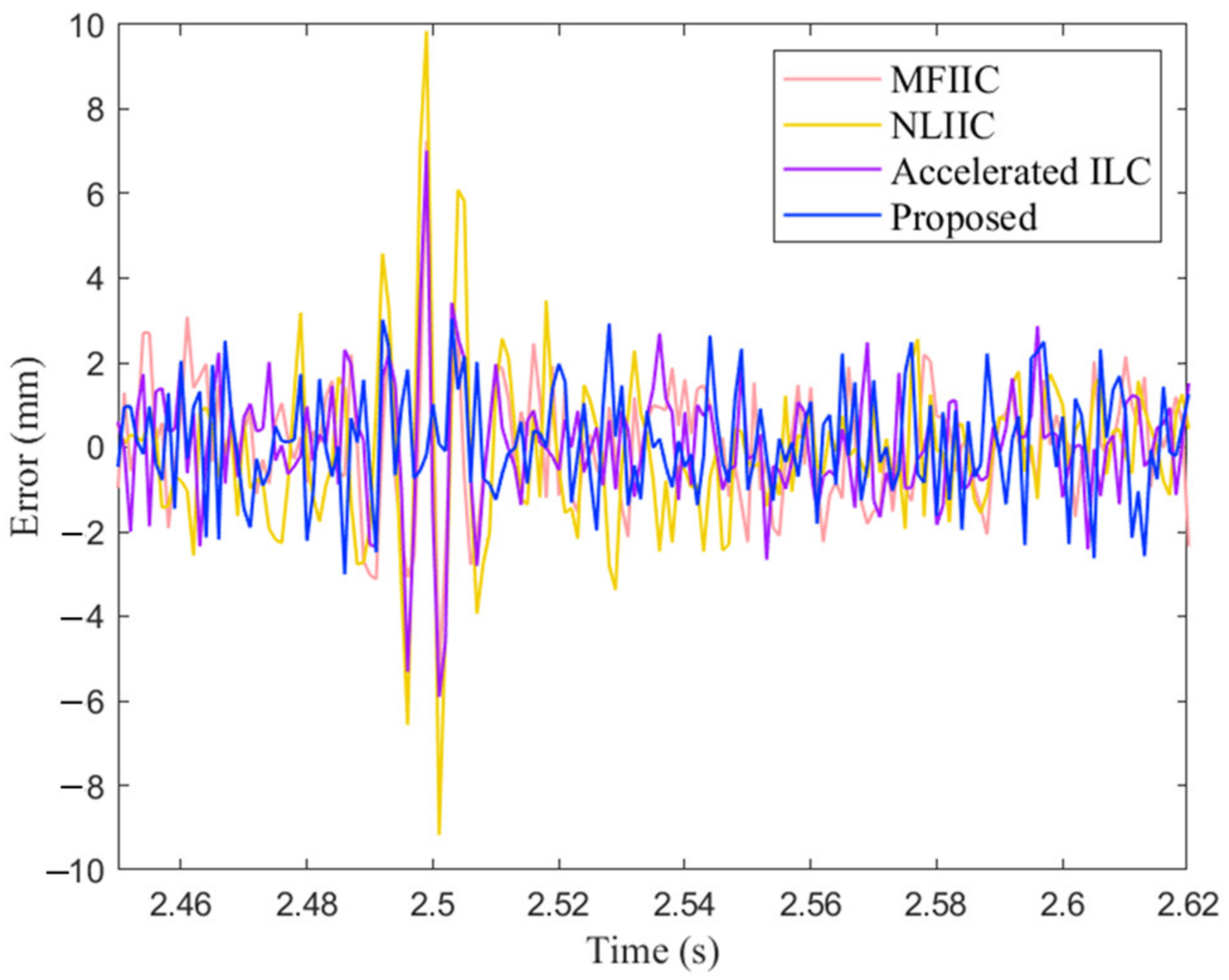
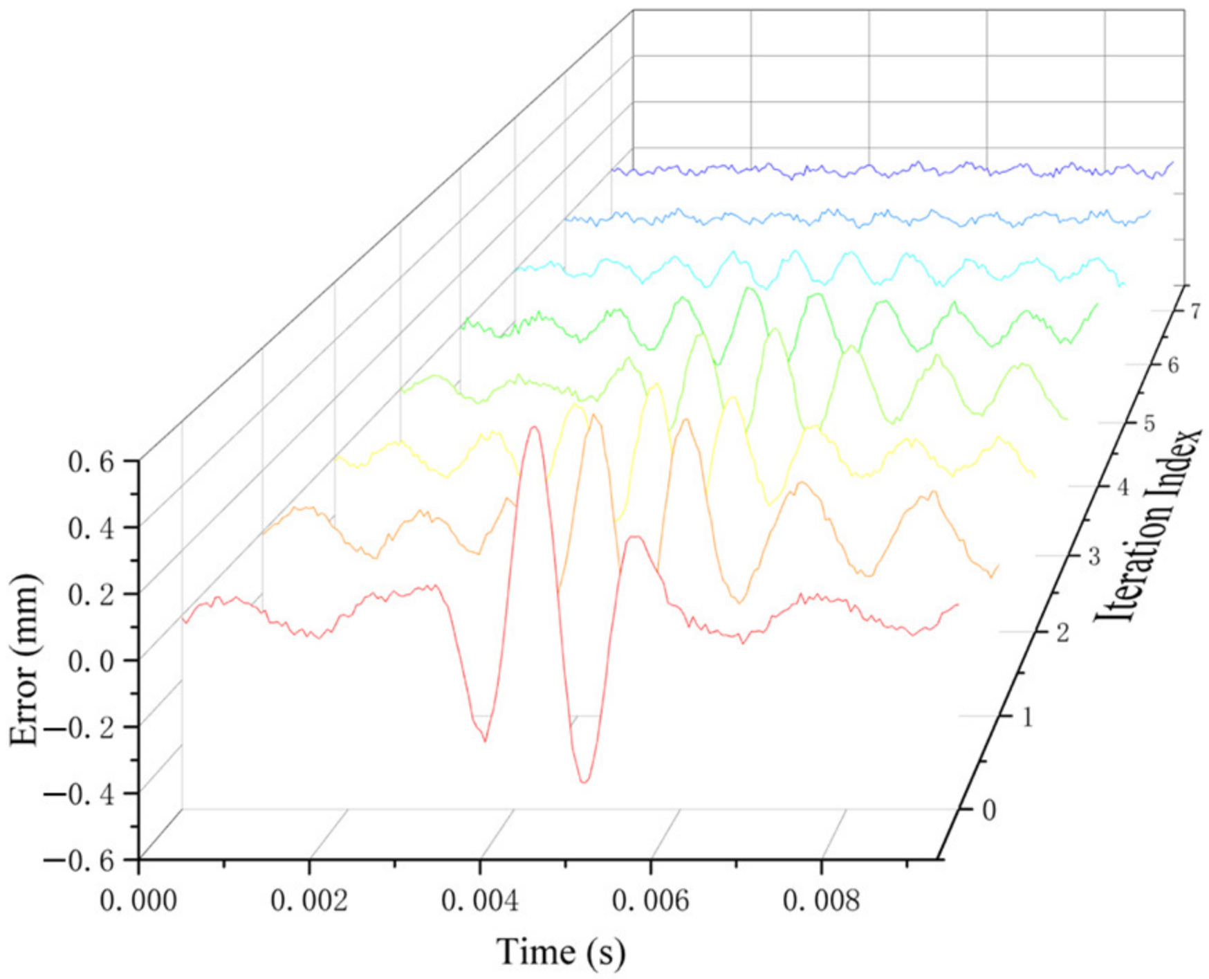
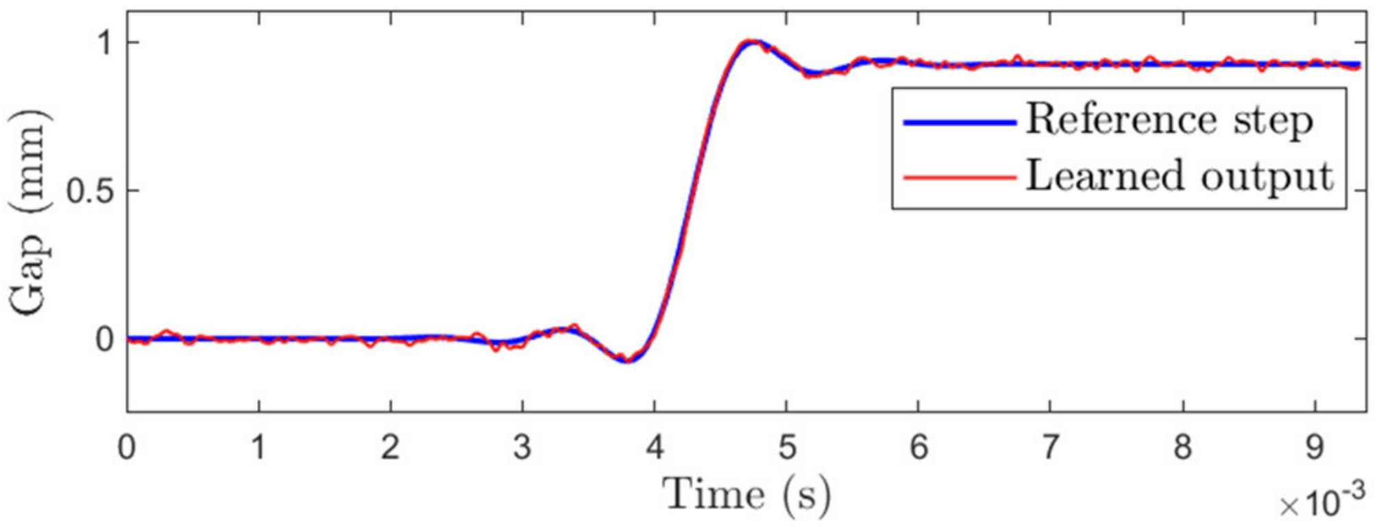
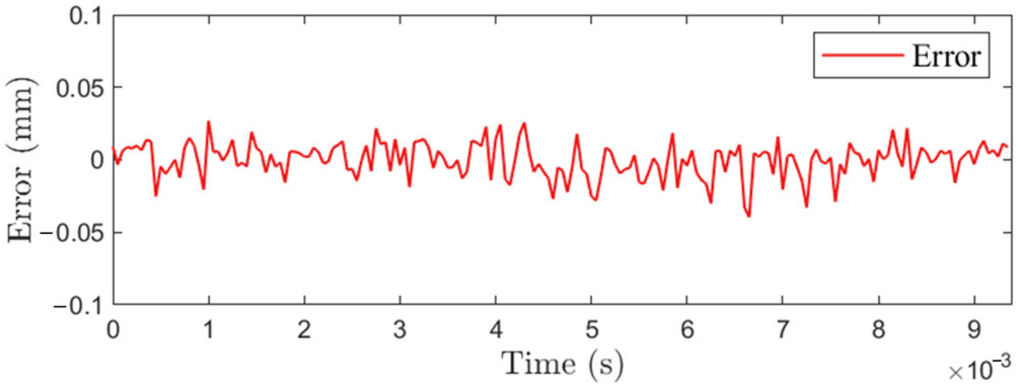
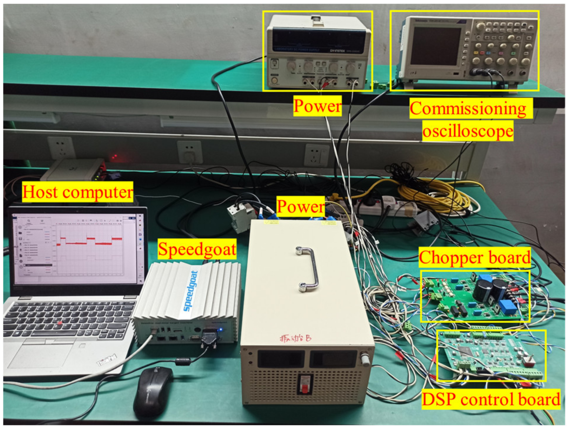
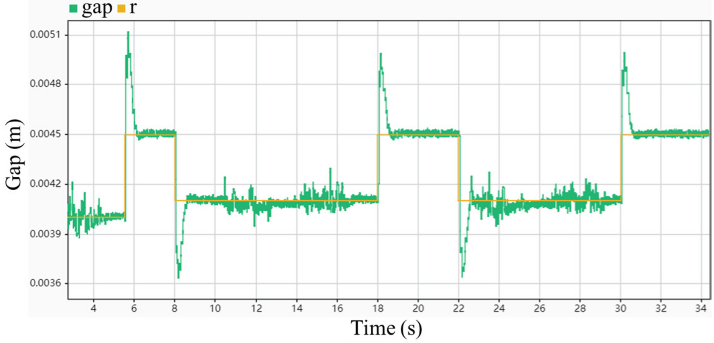
4. Suspension Control Experiment and Analysis

This section takes Changsha medium- and low-speed maglev trains as the research object, combines a large number of maglev train suspension gap data to realize the identification of the inverse model of the suspension system, and selects historical data with a high signal-to-noise ratio to improve the estimation accuracy.

The suspension clearance data of the maglev train is obtained through the data acquisition system. The data acquisition system is mainly composed of suspension gap sensor, acceleration sensor, current sensor, temperature sensor and corresponding data receiving and processing module. It can collect suspension gap, vertical acceleration, lateral acceleration, electromagnet working current and electromagnet coil surface temperature data during the operation of the maglev train, with a sampling rate of 1 kHz, as shown in Figure 6.

The prior information of the suspension system is used to improve the convergence speed of the data-driven nonlinear iterative inversion suspension control algorithm. The suspension system of maglev train after mechanical decoupling of suspension bogie is simplified as a single point suspension system, as shown in Figure 7.

Considering the single point suspension system of the maglev train, after linear processing at the suspension balance point, the state variable is $\left[\begin{array}{cc}\Delta z(t)& \Delta \dot{z}(t)\end{array}\right]$, and the state space description of the suspension system model can be obtained as follows [32]:

$$\{\begin{array}{l}\left[\begin{array}{c}\Delta \dot{z}\left(t\right)\\ \Delta \ddot{z}\left(t\right)\end{array}\right]=\left[\begin{array}{cc}0& 1\\ K_z/m& 0\end{array}\right]\left[\begin{array}{c}\Delta z\left(t\right)\\ \Delta \dot{z}\left(t\right)\end{array}\right]+\left[\begin{array}{c}0\\ -K_i/m\end{array}\right]\Delta u\left(t\right),\\ y\left(t\right)=\left[\begin{array}{ll}1\hfill & 0\hfill \end{array}\right]\left[\begin{array}{l}\Delta z\left(t\right)\hfill \\ \Delta \dot{z}\left(t\right)\hfill \end{array}\right],\end{array}$$

(38)

$$K_z=\frac{{\mu }_{0}S{N}^2{i}_0^2}{2z_0^3},K_i=\frac{{\mu }_{0}S{N}^2{i}_0}{2z_0^2},L_0=\frac{{\mu }_{0}S{N}^2}{2z_0}$$

(39)

where $\Delta i(t)$ is the change of coil current; $\Delta z(t)$ is the change of air gap; $\Delta u(t)$ is the change of the voltage at both ends of the solenoid coil. According to the data of Changsha maglev trains, vacuum permeability ${\mu }_0=12.6\times {10}^{-7}$ H/m, coil current $i_0=22.0$ A in steady state, time gap value in steady state $z_0=8.0$ mm, coil turns N = 360 turns, electromagnet sectional area S = 0.038 m², coil resistance R = 0.92 Ω, and electromagnet equivalent mass m = 535 kg. Therefore, the state space of the suspension system model describes the system matrix $A=\left[\begin{array}{cc}0& 1\\ 5467.52& 0\end{array}\right]$, control matrix $B=\left[\begin{array}{c}0\\ -1.99\end{array}\right]$, and output matrix $C=\left[\begin{array}{ll}1\hfill & 0\hfill \end{array}\right]$.

Then, a controller based on PID algorithm is designed to make the closed-loop stable. On the basis of this closed-loop single point suspension system model, considering the influence of track irregularity, a simulation experiment of nonlinear iterative inversion suspension control based on data drive is carried out [33,34]. After the suspension system simulation experiment, the iterative learning error curve is obtained, as shown in Figure 8. The system converges after finite iterative learning. It can be observed from the simulation experiment result curve that the error convergence speed of ILC based on time inversion is the slowest under the output noise interference environment with standard deviation of 1 mm and mean value of 0 mm. Compared with the ILC method based on time inversion, Accelerated Convergence Interleaving further improves the learning rate. The error convergence rate of MFIIC method is the fastest, but the method may have unpredictable learning transient for the case with output interference, as shown in Figure 9. NLIIC solves the robustness problem of MFIIC in the presence of output interference and has a fast error convergence rate. However, the steady-state tracking performance of NLIIC is worse than that of MFIIC and the methods proposed in this paper. As shown in Figure 10, at 2.5 s of the steady-state tracking error curve, NLIIC has a larger tracking error than other algorithms. The NLIIC method based on time inversion proposed in this paper has good steady-state tracking performance, and the iterative learning error convergence rate is fast, close to the error convergence rate of NLIIC.

The time domain tracking error after iterative learning is shown in Figure 10. According to Figure 11, when the number of updates of the learning filter increases, the tracking error of the system pulse response decreases. When the seventh learning filter update is completed, it can be considered that the FIR inverse filter at this time is superior to the previous results. The FIR inverse model is used to replace the learning filter, which achieves a faster error convergence rate [31].

Then the tracking control problem of the suspension system in the presence of track irregularity interference is studied. A step signal with Gaussian white noise interference is applied at the output position of the suspension system. After the suspension system simulation experiment, the step response simulation curve of the suspension system is obtained, as shown in Figure 12. It can be seen from Figure 12 that the suspension system can realize fast tracking control, and the tracking error of the system is within ±0.05 mm, as shown in Figure 13. The experimental results show that the data-driven nonlinear iterative inversion suspension control based on time inversion can achieve high-precision tracking control.

Finally, the tracking control experiment of the levitation system is carried out on the experimental platform of the magnetic levitation system. Verify the tracking control performance of the control algorithm designed in this paper in the presence of track irregularity interference. The control circuit module of the magnetic suspension vibration experimental platform is shown in Figure 14. The magnetic suspension vibration experiment platform includes the baseline series real-time target machine of Speedgoat Company (Bern, Switzerland), which realizes the real-time operation control and monitoring of the suspension system. The levitation electromagnet module and its corresponding control circuit board, chopper circuit board, upper computer and power supply module can simulate the levitation system of the maglev train. It also includes a vibrating table base module capable of applying external interference excitation. The suspension electromagnet module of the magnetic suspension system experimental platform is shown in Figure 15.

For the tracking control experiment of the suspension system, first of all, build the most commonly used closed-loop suspension control structure based on PID in engineering, adjust the PID parameters to make the system suspend stably, and obtain the experimental results of the step response output suspension gap curve of the closed-loop suspension system experiment based on PID algorithm without feedforward filter link, as shown in Figure 16. The control error curve of the step response experiment of the corresponding closed-loop suspension system is shown in Figure 17. At this time, the suspension control system can better follow the step input reference signal of the system but has a large overshoot. Then, on the basis of the closed-loop suspension control structure based on PID, the feedforward filter link of the data-driven nonlinear iterative inversion suspension control based on time inversion is added, and the suspension gap curve of the step response output of the data-driven nonlinear iterative inversion suspension control experiment with the feedforward filter link is obtained as shown in Figure 18. It can be seen from Figure 18 that after the results are updated iteratively, the system can track the step input reference signal well and has a small overshoot. The experimental results verify the effectiveness of the proposed method.

5. Conclusions

In this study, a data-driven nonlinear iterative inverse levitation control algorithm is designed for the levitation control of maglev train under track irregularity. According to the historical suspension clearance data of the suspension system, the model of the suspension system is identified in the iterative learning update process. The convergence of the control algorithm is analyzed when the system is subjected to bounded disturbance signals. Then, combining the advantages of NLIIC and MFIIC, the gain function of the control law is designed, and the control framework of the data-driven nonlinear iterative inversion levitation control algorithm is designed. Finally, the simulation experiment of the maglev train suspension system and the physical experiment of the maglev system experimental platform verify the high precision tracking performance of the suspension control algorithm proposed in this paper.

References

1. Hara, S.; Yamamoto, Y.; Omata, T.; Nakano, M. Repetitive control system: A new type servo system for periodic exogenous signals. IEEE Trans. Autom. Control. 1988, 33, 659–668. [Google Scholar] [CrossRef]
2. Teng, K.T.; Tsao, T.C. A comparison of inversion based iterative learning control algorithms. In Proceedings of the 2015 American Control Conference, Chicago, IL, USA, 1–3 July 2015; IEEE: Piscataway, NJ, USA, 2015; pp. 3564–3569. [Google Scholar]
3. Van Zundert, J.; Oomen, T. On inversion-based approaches for feedforward and ILC. Mechatronics 2018, 50, 282–291. [Google Scholar] [CrossRef]
4. Lee, K.S.; Bang, S.H.; Chang, K.S. Feedback-assisted iterative learning control based on an inverse process model. J. Process Control 1994, 4, 77–89. [Google Scholar] [CrossRef]
5. Kinosita, K.; Sogo, T.; Adachi, N. Iterative learning control using adjoint systems and stable inversion. Asian J. Control 2002, 4, 60–67. [Google Scholar] [CrossRef]
6. De Roover, D.; Bosgra, O.H. Synthesis of robust multivariable iterative learning controllers with application to a wafer stage motion system. Int. J. Control. 2000, 73, 968–979. [Google Scholar] [CrossRef]
7. Amann, N.; Owens, D.H.; Rogers, E.; Wahl, A. An H∞ approach to linear iterative learning control design. Int. J. Adapt. Control Signal Process. 1996, 10, 767–781. [Google Scholar] [CrossRef]
8. Hou, Z.S.; Wang, Z. From model-based control to data-driven control: Survey, classification and perspective. Inf. Sci. 2013, 235, 3–35. [Google Scholar] [CrossRef]
9. Chi, R.; Huang, B.; Wang, D.; Zhang, R.; Feng, Y. Data-driven optimal terminal iterative learning control with initial value dynamic compensation. IET Control Theory Appl. 2016, 10, 1357–1364. [Google Scholar] [CrossRef]
10. Chi, R.; Wang, D.; Hou, Z.; Jin, S. Data-driven optimal terminal iterative learning control. J. Process Control 2012, 22, 2026–2037. [Google Scholar] [CrossRef]
11. Bolder, J.; Kleinendorst, S.; Oomen, T. Data-driven multivariable ILC: Enhanced performance by eliminating L and Q filters. Int. J. Robust Nonlinear Control 2018, 28, 3728–3751. [Google Scholar] [CrossRef]
12. Janssens, P.; Pipeleers, G.; Swevers, J. Model-free iterative learning control for LTI systems and experimental validation on a linear motor test setup. In Proceedings of the 2011 American Control Conference, San Francisco, CA, USA, 29 June–1 July 2011; IEEE: Piscataway, NJ, USA, 2011; pp. 4287–4292. [Google Scholar]
13. Kim, K.S.; Zou, Q. A modeling-free inversion-based iterative feedforward control for precision output tracking of linear time-invariant systems. IEEE/ASME Trans. Mechatron. 2012, 18, 1767–1777. [Google Scholar] [CrossRef]
14. Janssens, P.; Pipeleers, G.; Swevers, J. A data-driven constrained norm-optimal iterative learning control framework for LTI systems. IEEE Trans. Control Syst. Technol. 2012, 21, 546–551. [Google Scholar] [CrossRef]
15. Boeren, F.; Oomen, T.; Steinbuch, M. Iterative motion feedforward tuning: A data-driven approach based on instrumental variable identification. Control Eng. Pract. 2015, 37, 11–19. [Google Scholar] [CrossRef]
16. Feng, Z.; Ling, J.; Ming, M.; Xiao, X. A model-data integrated iterative learning controller for flexible tracking with application to a piezo nanopositioner. Trans. Inst. Meas. Control 2018, 40, 3201–3210. [Google Scholar] [CrossRef]
17. Wang, Z.; Zou, Q. A modeling-free differential-inversion-based iterative control approach to simultaneous hysteresis-dynamics compensation: High-speed large-range motion tracking example. In Proceedings of the 2015 American Control Conference, Chicago, IL, USA, 1–3 July 2015; IEEE: Piscataway, NJ, USA; pp. 3558–3563. [Google Scholar]
18. Devasia, S. Iterative machine learning for output tracking. IEEE Trans. Control Syst. Technol. 2017, 27, 516–526. [Google Scholar] [CrossRef]
19. Ito, S.; Yoo, H.W.; Schitter, G. Comparison of modeling-free learning control algorithms for galvanometer scanner’s periodic motion. In Proceedings of the 2017 IEEE International Conference on Advanced Intelligent Mechatronics, Munich, Germany, 3–7 July 2017; IEEE: Piscataway, NJ, USA; pp. 1357–1362. [Google Scholar]
20. De Rozario, R.; Oomen, T. Data-driven iterative inversion-based control: Achieving robustness through nonlinear learning. Automatica 2019, 107, 342–352. [Google Scholar] [CrossRef]
21. Bolder, J.; Oomen, T. Rational basis functions in iterative learning control—With experimental verification on a motion system. IEEE Trans. Control Syst. Technol. 2014, 23, 722–729. [Google Scholar] [CrossRef]
22. Gao, X.; Mishra, S. An iterative learning control algorithm for portability between trajectories. In Proceedings of the 2014 American Control Conference, Portland, OR, USA, 4–6 June 2014; IEEE: Piscataway, NJ, USA, 2014; pp. 3808–3813. [Google Scholar]
23. Blanken, L.; Hazelaar, T.; Koekebakker, S.; Oomen, T. Multivariable repetitive control design framework applied to flatbed printing with continuous media flow. In Proceedings of the 2017 IEEE 56th Annual Conference on Decision and Control, Melbourne, Australia, 12–15 December 2017; IEEE: Piscataway, NJ, USA, 2017; pp. 4727–4732. [Google Scholar]
24. Moore, K.L. Iterative Learning Control for Deterministic Systems; Springer: Berlin/Heidelberg, Germany, 2012. [Google Scholar]
25. Devasia, S.; Chen, D.; Paden, B. Nonlinear inversion-based output tracking. IEEE Trans. Autom. Control 1996, 41, 930–942. [Google Scholar] [CrossRef]
26. Zeng, G.; Hunt, L.R. Stable inversion for nonlinear discrete-time systems. IEEE Trans. Autom. Control 2000, 45, 1216–1220. [Google Scholar] [CrossRef]
27. Chen, C.W.; Tsao, T.C. Accelerated convergence interleaving iterative learning control and inverse dynamics identification. IEEE Trans. Control Syst. Technol. 2021, 30, 45–56. [Google Scholar] [CrossRef]
28. Blanken, L. Learning and Repetitive Control for Complex Systems: With Application to Large-Format Printers. Ph.D. Thesis, Eindhoven University of Technology, Eindhoven, The Netherlands, 2019. [Google Scholar]
29. De Rozario, R. Data-Driven Learning Control for Complex Multivariable and Linear Parameter-Varying Systems. Ph.D. Thesis, Eindhoven University of Technology, Eindhoven, The Netherlands, 2020. [Google Scholar]
30. Zhang, G.H.; Chen, C.W. On Improving Transient Behavior and Steady-State Performance of Model-free Iterative Learning Control. IFAC—Pap. 2020, 53, 1433–1438. [Google Scholar] [CrossRef]
31. Chen, C.W.; Rai, S.; Tsao, T.C. Iterative learning of dynamic inverse filters for feedforward tracking control. IEEE/ASME Trans. Mechatron. 2019, 25, 349–359. [Google Scholar] [CrossRef]
32. Long, Z.Q.; Hao, A.M.; Chang, W.S. Suspension controller design of maglev train considering the rail track periodical irregularity. J. Natl. Univ. Def. Technol. 2003, 025, 84–89. [Google Scholar]
33. Havaei, P.; Sandidzadeh, M.A. Intelligent-PID controller design for speed track in automatic train operation system with heuristic algorithms. J. Rail Transp. Plan. Manag. 2022, 22, 100321. [Google Scholar] [CrossRef]
34. Witanowski, Ł.; Breńkacz, Ł.; Szewczuk-Krypa, N.; Dorosińska-Komor, M.; Puchalski, B. Comparable analysis of PID controller settings in order to ensure reliable operation of active foil bearings. Eksploat. Niezawodn. 2022, 24, 377–385. [Google Scholar] [CrossRef]
Figure 1. Vertical section of maglev commercial operation line project.
Actuators 12 00068 g001
Figure 2. Cross section diagram of track beam structure in curved section of maglev commercial operation line.
Actuators 12 00068 g002
Figure 3. Suspension control block diagram of nonlinear IIC based on data-driven.
Actuators 12 00068 g003
Figure 4. Schematic diagram of gain switching structure of control algorithm learning law proposed in this paper.
Actuators 12 00068 g004
Figure 5. Schematic diagram of control algorithm learning filter updating structure proposed in this paper.
Actuators 12 00068 g005
Figure 6. Schematic diagram of maglev data system.
Actuators 12 00068 g006
Figure 7. Schematic diagram of single point suspension system of maglev train.
Actuators 12 00068 g007
Figure 8. Error curve of iterative learning process.
Actuators 12 00068 g008
Figure 9. Error curve of iterative learning process.
Actuators 12 00068 g009
Figure 10. Steady state levitation tracking error curve.
Actuators 12 00068 g010
Figure 11. Pulse response tracking error curve after learning filter updating.
Actuators 12 00068 g011
Figure 12. Simulation curve of suspension system step response.
Actuators 12 00068 g012
Figure 13. Suspension system tracking control error curve.
Actuators 12 00068 g013
Figure 14. Schematic diagram of control circuit module of magnetic suspension system experimental platform.
Actuators 12 00068 g014
Figure 15. Schematic diagram of suspension electromagnet module of magnetic suspension system experimental platform.
Actuators 12 00068 g015
Figure 16. Suspension clearance curve of step response output of closed-loop suspension system experiment based on PID algorithm without feedforward filter link.
Actuators 12 00068 g016
Figure 17. Control error curve of step response of closed-loop suspension system experiment based on PID algorithm without feedforward filter link.
Actuators 12 00068 g017
Figure 18. Suspension gap curve of step response output of suspension control experiment based on time driven nonlinear iterative inversion with feedforward filter link.
Actuators 12 00068 g018
Disclaimer/Publisher’s Note: The statements, opinions and data contained in all publications are solely those of the individual author(s) and contributor(s) and not of MDPI and/or the editor(s). MDPI and/or the editor(s) disclaim responsibility for any injury to people or property resulting from any ideas, methods, instructions or products referred to in the content.