Abstract
To address system parameter changes during permanent magnet synchronous motor (PMSM) operation, an H∞ filtering algorithm with a dynamic forgetting factor is proposed for online identification of motor resistance and inductance. First, a standard linear discrete PMSM parameter identification model is established; then, the discrete H∞ filtering algorithm is derived using game theory reducing state and measurement noise influence. A cost function is defined, solving extremes values of different terms. A dynamic forgetting factor is introduced to the weighted combination of initial and current measurement noise covariance matrices, eliminating identification issues from different initial values. On this basis, a dynamic forgetting factor is added to weigh the combination of the initial measurement noise covariance matrix and the current measurement noise covariance matrix, which eliminates the influence of the discrimination error caused by the different initial values. Finally, the identification model is built in MATLAB/Simulink for simulation analysis to verify the feasibility of the proposed algorithm. The simulation results show the proposed H∞ filtering algorithm rapidly and accurately identifies resistance and inductance values with significantly improved robustness. The forgetting factor enables quick stable recognition even with poor initial values, enhancing PMSM control performance.
1. Introduction
The structure of a permanent magnet synchronous motor and other factors can result in differences in motor parameters under different working conditions. This can reduce the accuracy of the overall control system and potentially impact system stability []. Accurate identification of motor parameters is therefore crucial.
Compared to offline identification methods, ideal online methods can accurately estimate motor parameters in real time, enhancing system control performance [,,]. Current online parameter identification methods for permanent magnet synchronous motors primarily utilize least squares [,,], model reference adaptive [,,], and Kalman filter algorithms [,,]. Uddin et al. [] realizes online alternating axis inductance by identification via a model-referenced adaptive algorithm, assuming known, constant stator resistance and permanent magnet magnetic chain. Gao et al. [] proposed a model-referenced adaptive system based on disturbance compensation, designed a real-time disturbance estimator, and updated the adaptive rate according to the disturbance. This reduces system uncertainty and disturbance effects and increases model-referenced adaptive algorithm application scenarios. Based on the permanent magnet synchronous motor mechanical and electromagnetic models, Tang et al. [] designed an adaptive rate improvement model reference adaptive algorithm. This estimates rotor position and load torque while designing a load torque feedforward compensator controller for quick load response. Kalman filtering for linear systems can be updated in real-time to optimally estimate parameters but often fails with unknown noise and large modeling errors. The motor system is nonlinear, so many scholars improved Kalman filtering, such as via extended Kalman filtering [,], traceless Kalman filtering [], unscented Kalman filtering [], etc. Kalman filtering assumes Gaussian distributed measurement noise, but system noise statistics are often unknown or time-varying in reality. The adaptive Kalman filtering algorithm in reference [] addresses this to some extent by selecting the appropriate covariance distribution to estimate the covariance matrix, which does not vary significantly. However, it is limited by the linear Gaussian state model. Researchers have achieved many achievements in engine parameter identification, but existing methods often only consider Gaussian noise, while practice engines are often disturbed by non-Gaussian noise and other factors. For Gaussian noise with unknown covariance, the traditional H∞ filtering algorithm is used. Chen et al. [] proposes an adaptive H∞ filtering algorithm for parameter identification, based on the traditional extended H∞ filtering algorithm, and investigates the online identification of motor stator inductance and resistance. However, the covariance of the traditional H∞ filtering algorithm is set by humans, which affects the accuracy of the H∞ filtering algorithm. As inductance parameters are influenced by the motor’s operating state, Liu et al. [] establishes a motor model based on the motor’s transient voltage equation and introduces a forgetting factor to improve the least squares identification method, successfully enhancing algorithm tracking performance. However, setting the forgetting factor to a specific value makes ensuring the least squares method’s robustness during identification difficult. Fang et al. [] takes the error between theoretical and actual output as a variable, dynamically adjusting the forgetting factor, to accelerate algorithm convergence and ensure robustness.
Therefore, this paper proposes a discrete H∞ filtering algorithm containing dynamic forgetting factor based on minimizing maximum estimation error requiring no assumptions about system or observation noise characteristics. The remaining paper is organized as follows: First, a PMSM parameter identification model is established from the PMSM’s d-q mathematical model. Second, the cost function is defined per H∞ filtering, with the extreme point solved. Then, a dynamic forgetting factor is introduced to reduce abnormal initial value influence on the algorithm. Finally, this H∞ filtering with dynamic forgetting factor identifies PMSM parameters, verifying effectiveness via simulation.
2. Modeling of PMSM Parameter Identification
To facilitate the study, the mathematical model under the synchronous rotation coordinate system d-q of the permanent magnet synchronous motor is usually selected, so that the stator voltage equation can be expressed as
The equation for the stator chain can be expressed as follows:
Substituting Equation (2) into Equation (1) gives the following Equation:
where ud and uq are the voltages of the d and q axes, respectively; id and iq are the currents of the d and q axes, respectively; Rs is the stator resistance; Ψd and Ψq are the stator chain components, respectively; ωe is the electric angular velocity of the rotor; Ld and Lq are the inductances of the d and q axes, respectively; and Ψf is the magnetic chain of the permanent magnet.
The state space equations for the permanent magnet synchronous motor are established by selecting the id and iq of the current in the d and q axes and identifying the parameters Ld and Lq, and Rs as state variables. This paper focuses on the surface-mounted motor, which satisfies Ld = Lq = Ls. Thus, Equation (3) can be rearranged as follows:
Since the coefficient matrix of Equation (4) contains coupling terms, the direct identification of Rs and Ls becomes more complex. Therefore, intermediate variables a and b are introduced to simplify the identification equations. Let a = Rs/Ls, b = 1/Ls. Equation (4) can be rearranged as follows:
The output y can be expressed as
where w represents the process noise of the system and v represents the measurement noise of the system. The state variable matrix of the system is denoted by x = [id iq a b]T, and the output variable matrix is denoted by y = [id iq]T. By discretizing Equations (5) and (6) using the sampling period Ts, the standard linear discrete system form presented below is obtained as
where wk and vk are noise terms that are random and of unknown statistical properties; Fk and Hk represent the coefficient matrices as follows:
Thus, the algorithm in this study uses the H∞ filtering algorithm to detect parameters a and b using the above model. Next, the values of resistance Rs and inductance Ls are obtained by relating a and b and Rs and Ls.
3. H∞ Filtering Algorithm Based on Game Theory
The estimation of xk is denoted as k, and the estimation of the initial state is denoted as 0. In the game-theoretic approach to derive H∞ filtering and estimate xk, including N − 1 moments and N − 1 moments before the measurement condition, the cost function [] must be defined as shown in Equation (9):
The presence of disturbances, such as natural noise, produces wk, vk, and x0, that maximizes J1. Thus, the cost function places wk, vk and x0 in the denominator. To minimize J1, we must estimate xk in the cost function and find the appropriate solution. Equation (9) employs symmetric positive definite matrices P0, Qk, Rk and Sk, chosen based on the specific problem.
Minimizing J1 directly is challenging; thus, we choose a performance limit that ensures the J1 cost function meets the following condition:
θ is the performance boundary. We set the following:
Therefore, from Equation (11), it can be seen that J can be minimized by choosing an appropriate wk, vk, and x0, while wk, vk, and x0 generated by the noise effect can maximize J. The noise effect can be expressed by substituting vk into Equation (11). From yk = Hkxk + vk in Equation (7), it can be seen that vk = yk − Hkxk, and substituting vk into Equation (11) can be expressed as
where Ψ(x0) and Lk can be expressed by Equation (13), and to solve the extreme-problem that exists in Equation (12), the extreme points of J with respect to wk and x0 can be found first, and then the extreme points of J with respect to k and yk.
3.1. Extreme Solutions for wk and x0
To obtain the maximum value with respect to J, we define the Hamiltonian function as follows:
The 2λTk+1/θ is the time-varying Lagrange multiplier to be computed (k = 0,…, N − 1). It is clear from the theory of dynamic constrained optimization that we can solve the constrained optimization problem of J with respect to wk and x0 via the following Equation:
Simplified Equation (15):
This can be obtained by substituting wk = Qkλk+1 in Equation (16) into Equation (7):
From Equation (16), we obtain x0 = 0 + P0λ0, so we can set that
Equation (18) holds for all k. μk and Pk are functions to be determined, P0 is given, and the initial value μ0 = 0. Assume that xk is an affine function of λk, if the final result is correct, our assumption is correct. Substituting Equation (18) into Equation (17), we obtain
Substituting λk = FkTλk+1 + θSk(xk − k) + HkTRk−1(yk − Hkxk) in Equation (16) into Equation (18), we obtain
Shifting the terms gives λk as follows:
Substituting the expression of Equation (21) into Equation (19) gives the following:
This equation holds when both sides of the above equation are zero at the same time. Setting the left side to zero gives:
Let the right side of Equation (22) be zero to obtain
Define k as
It follows from Equation (25) that if Pk, Sk, and Rk are symmetric, then they will also be positive definite; and it follows from Equation (24) that if Qk is positive definite, then Pk+1 will also be positive definite; so, for all k, P0, Sk, Qk, and Rk, if they are all symmetric, then k and Pk will be symmetric at some point.
It turns out that we are able to find the extreme points of J, so the above assumption is correct. Using the values of x0 and wk already obtained, we can again find the extreme points of the function J with respect to k and yk.
3.2. Extreme Solutions for and
Based on the solution of the problem of the extreme points of x0 and wk, we also need to find the extreme points of the function J with respect to k and yk. From the initial condition of μk in Equation (18), we can see that
The following can be obtained from Equation (26):
In this case, Equation (12) can be rewritten as
Substituting the expression for xk, the Equation (28) can be rewritten as
Substituting the expression for wk in Equation (16) into this position of Equation (29) gives the new equation:
As Qk is a symmetric matrix, Equation (30) can be written as
It follows from Equation (16) that λN = 0; hence,
Equation (32) can be written as
Equation (31) is obtained by subtracting Equation (33) and simplifying the following:
Taking Equation (24) into Equation (34) and organizing it gives the following:
Taking Equation (35) into Equation (34) and organizing it gives the following:
The goal is to find the solutions to the extreme value problem of J with respect to k and yk. Therefore, the J of Equation (36) is made to take partial derivatives with respect to k and yk, respectively, and the partial derivatives are made to be zero. We obtain the following:
The solutions to Equation (37) are as follows:
k and yk in Equation (38) are the extreme points of Equation (37). If the second-order partial derivatives of J are positive definite, it means that the extreme point is the minimum point. The second-order partial derivatives of J with respect to k are as follows:
If Sk + θSkkSk is positive definite, k will be the point where J is minimized. The choice of Sk in Equation (9) is always positive definite, so k will be the point of minimum of J as long as k is positive definite.
From Equations (23), (24) and (38), a filtering method as shown in Equation (40) can be derived such that the cost function J1 can be smaller than 1/θ.
where Kk is the gain matrix.
In order to have a solution to the problem of the observer of Equation (40), the following conditions must always be satisfied:
4. Forgetting Factor H∞ Filtering Algorithm
In the H∞ filtering algorithm, the noise covariance matrix is artificially set based on experience, and its initial value affects the accuracy and convergence of the algorithm [,,]. In this chapter, assuming a fixed process noise covariance matrix, we design a dynamic forgetting factor to weight the combination of the initial and current measurement noise covariance matrices. The initial matrix is gradually forgotten to minimize the effect of anomalous initial values on the algorithm.
Define the best estimate of the measurement noise via the following:
Combined with Equation (7), these yield the following:
At this point, the measurement noise covariance matrix is as follows:
Define the dynamic forgetting factor βk:
where α is a constant, usually taken as 0.96~0.99.
Weighting the measurement noise covariance matrix with a dynamic forgetting factor strengthens the role of the measurement noise covariance matrix in the estimation at that moment and gradually forgets the initial measurement noise covariance matrix:
Combining Equation (46) with the filtering method shown in Equation (40) can lead to the H∞ filtering algorithm with dynamic forgetting factor shown in Equation (47):
5. Experimental Analysis and Comparison
In order to verify the feasibility of the parameter identification algorithm proposed in this paper, relevant simulations are carried out in this chapter to verify the simulation flowchart, and the motor parameters used are shown in Figure 1 and Table 1.
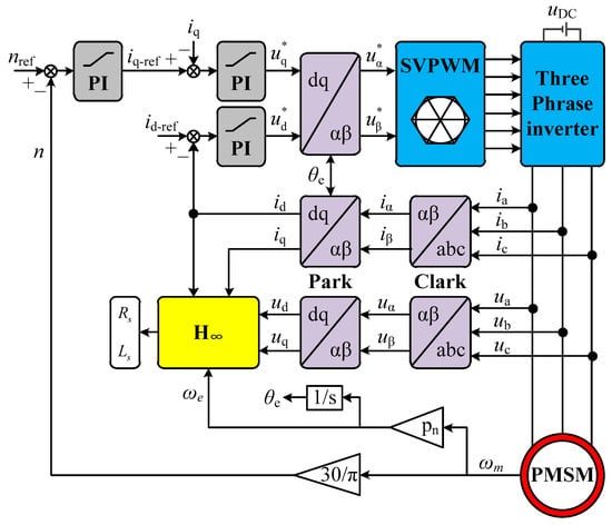
Figure 1.
Permanent magnet synchronous motor system model.

Table 1.
Parameters of the PMSM control system.
In this section, the parameter identification simulation under a steady-state condition is carried out first to verify the effectiveness of the proposed identification algorithm then to verify the robustness of the proposed parameter identification algorithm, the simulation analysis is carried out for three conditions of motor load change, stator resistance change, and stator inductance change in turn. At the end, the effectiveness of the parameter identification algorithm with the addition of a forgetting factor is verified.
5.1. Steady-State Performance
The motor is operating in a steady-state condition. The motor load is set to 0.3 N·m and the motor speed is set to 600 rpm. The parameters of the recognition algorithm are set as follows: x0 = [0.01 5 280 550], P0 = diag([0.01 0.1 1 1]), Sk = diag([0.18 0.06 0 0]), Qk = diag([0 0 0.9 1.18]),and Rk = [1 1], Ts = 0.0001 s. The simulation results are shown in Figure 2.
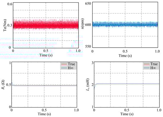
Figure 2.
Parameter identification of Rs and Ls under steady-state conditions.
From Figure 2, it can be seen that the proposed parameter identification algorithm can achieve the identification of resistance and inductance in a short time. The difference between the final identification result and the actual value of the resistance is almost 0. The actual value of the inductance is 2 mH, the final identification is 2.1 mH, and the difference between the final identification result and the actual value of inductance is within 5%, which proves the effectiveness of the proposed parameter identification algorithm.
5.2. Robustness Verification
5.2.1. Load Torque
The motor speed is set to 900 rpm and the torque changes from 0.2 N·m to 0.4 N·m at 0.5 s. The simulation results are shown in Figure 3.
Figure 3.
Parameter identification of Rs and Ls under load torque variation.
From Figure 3, it can be seen that the proposed parameter identification algorithm can guarantee the identification of the parameters when the torque is changed (twice). The resistance parameter identification results remain almost unchanged when the torque is changed. The inductance parameter identification results are 2.2 mH and 2.1 mH, respectively, and the difference between the changed identification result and the previous one is within 2%, which proves that the proposed parameter identification algorithm is robust to the torque-change condition.
5.2.2. Stator Resistance
In this subsection, the simulation simulates two operating conditions: sudden change in resistance due to motor failure and slow increase in resistance due to temperature rise and other factors. The stator resistance increased stepwise from 0.48 Ω to 0.8 Ω and gradually to 0.8 Ω, respectively. The motor speed is set to 900 rpm, the motor load is set to 0.3 N·m, and the simulation results are shown in Figure 4.
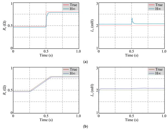
Figure 4.
Parameter identification of Rs and Ls under varying stator resistance: (a) sudden change in resistance due to motor failure; (b) slow increase in resistance due to temperature rise and other factors.
From Figure 4, it can be seen that the proposed parameter identification algorithm can guarantee the identification of the parameters when the resistance is changed and guarantees the qualified response speed when the resistance is changed abruptly, which proves that the proposed parameter identification algorithm connects the robustness to the working condition of the resistance change.
5.2.3. Stator Inductance
In this section, the simulation simulates the inductance change condition corresponding to the previous section. The stator inductance is abruptly changed from 2 mH to 4 mH and gradually increases from 2 mH to 4 mH. The motor speed is set to 900 rpm, the motor load is set to 0.3 N·m, and the simulation results are shown in Figure 5.
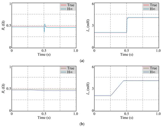
Figure 5.
Parameter identification of Rs and Ls under varying stator inductance. (a) The stator inductance changed abruptly from 2 mH to 4 mH. (b) The stator inductance changed gradually from 2 mH to 4 mH.
From Figure 5, it can be seen that the proposed parameter identification algorithm can guarantee the identification of the parameters when the inductance is changed and guarantees the qualified response speed when the inductance is changed abruptly, which proves that the proposed parameter identification algorithm connects the robustness to the working condition of the inductance change.
5.3. Validation of the Forgetting Factor
In this section, the steady-state condition of Section 5.1 is re-simulated for the identification algorithm before and after adding the forgetting factor. Then, the R matrix is changed to [10 10] to verify the effectiveness of the forgetting factor proposed in this paper. The comparative simulation results are shown in Figure 6.
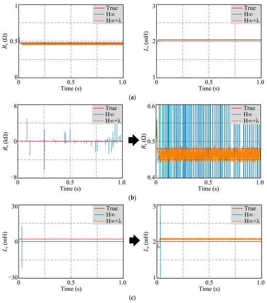
Figure 6.
Comparison of the effect of parameter identification after adding forgetting factor. (a) The condition of steady-state. (b) Identification of parameter Rs when the initial value is abnormal. (c) Identification of parameter Ls when the initial value is abnormal.
From Figure 6, it can be seen that the recognition algorithm with the added forgetting factor is not much different from the previous algorithm when the initial parameters are normal. However, when the initial parameters are abnormal, the observation results of the recognition algorithm without the added forgetting factor are abnormal, while the proposed forgetting factor is able to correct the error and recognize the parameters in time.
6. Discussion
With the development of modern power electronics technology, PMSMs are increasingly used in CNC machine tools, robots, and new energy vehicles due to their simple structure, high efficiency, and high functionality. However, there are modeling errors and noise uncertainties in PMSM systems. To meet the system’s requirements for robustness, we adopt the H∞ filtering algorithm. However, the noise covariance matrix and the upper performance limit of the H∞ filtering algorithm are set empirically, which may affect the accuracy of the algorithm. If they are not set appropriately, it may lead to a decrease in system accuracy and even to filtering divergence.
The application of the H∞ filtering algorithm to real PMSMs requires online identification of several parameters, such as motor speed, rotor position, and magnetic chain. These parameters will be collected by measuring instruments in the motor system and processed by the H∞ filtering algorithm, which reduces the influence of noise and other external disturbances, achieving high-accuracy online parameter identification of the motor and improving system robustness. However, implementing the H∞ filtering algorithm in a real PMSM system faces many challenges.
- (1)
- Sensor noise: The PMSM control system uses sensors to obtain measured values of the motor state, which may contain sensor noise. The H∞ filtering algorithm must consider the influence of sensor noise when dealing with external noise interference. If the statistical characteristics of the sensor noise change, the accuracy of the H∞ filtering algorithm may be affected.
- (2)
- High sampling rate and data processing requirements: Servo motors are generally divided into three control rings-current, speed, and position. The frequency of each ring determines its position, with higher frequencies corresponding to inner rings. PMSM control systems require high sampling rates for accurate measurement and control, increasing hardware and real-time performance requirements. Additionally, H∞ filtering may need to process large amounts of data, which is challenging for devices with limited data processing capabilities.
7. Conclusions
Through theoretical analysis and simulation verification, it can be concluded that the H∞ filtering algorithm based on game theory can obtain the recognition results quickly and accurately without making any assumptions about the noise, and its robustness has been significantly improved. The H∞ filtering algorithm after adding the improved forgetting factor can quickly and stably obtain the recognition result under the situation of poor initial value, which compensates the recognition error caused by human setting.
The algorithm proposed in this paper improves the estimation accuracy and robust performance of the original algorithm to some extent, but there are still deficiencies to be improved:
- (1)
- This paper improves the H∞ filtering algorithm by adding a dynamic forgetting factor, achieving weighted estimation of the initial and current measurement noise covariances. Although the accuracy of the algorithm is improved, it takes more time due to multiple iterations per time step.
- (2)
- The motor in the simulation ran at low speed, and the algorithm is inadequate for high-speed operation. The subsequent work can focus on identifying motor parameters during high-speed operation.
Author Contributions
Conceptualization, T.Y., J.C. and Y.Z.; methodology, J.C.; software, J.C. and Y.Z.; validation, T.Y., J.C. and Y.Z.; formal analysis, T.Y., J.C. and Y.Z.; investigation, T.Y.; resources, T.Y.; data curation, Y.Z.; writing—original draft preparation, J.C. and Y.Z.; writing—review and editing, J.C. All authors have read and agreed to the published version of the manuscript.
Funding
This research was funded by the project is supported by Scientific Research Project of Education Department of Jilin Province (No. JJKH20230121KJ).
Data Availability Statement
Data are contained with the article.
Conflicts of Interest
The authors declare no conflict of interest.
References
- Ali, N.; Alam, W.; Pervaiz, M.; Iqbal, J. Nonlinear adaptive backsteepping control of permanent magnet synchronous motor. RRST-EE 2023, 66, 15–20. [Google Scholar]
- Zhang, X.H.; Zhao, J.W.; Wang, L.J.; Hu, D.B.; Wang, L. High Precision Anti-interference Online Multiparameter Estimation of PMSLM With Adaptive Interconnected Extend Kalman Observer. Proc. CSEE 2022, 12, 4571–4581. [Google Scholar]
- Ma, Y.L.; Yuan, H.; Yin, W.; Yang, H. An on-line parameter identification method for PMSM DC signal injection considering equivalent electromagnetic loss resistance offset. Trans. China Electrotech. Soc. 2023, 6015–6026. [Google Scholar]
- Zhang, Q.S.; Fan, Y. The Online Parameter Identification Method of Permanent Magnet Synchronous Machine under Low-Speed Region Considering the Inverter Nonlinearity. Energies 2022, 15, 4314. [Google Scholar] [CrossRef]
- Yu, J.W. Research on Online Parameter Identification of Permanent Magnet Synchronous Motor Considering the Variation of Operating Condition; Harbin Institute of Technology: Harbin, China, 2021. [Google Scholar]
- Lian, C.Q.; Xiao, F.; Liu, J.L.; Gao, S. Parameter and VSI Nonlinearity Hybrid Estimation for PMSM Drives Based on Recursive Least Square. IEEE Trans. Transp. Electrif. 2023, 9, 2195–2206. [Google Scholar] [CrossRef]
- Purbowaskito, W.; Wu, P.Y.; Lan, C.Y. Permanent Magnet Synchronous Motor Driving Mechanical Transmission Fault Detection and Identification: A Model-Based Diagnosis Approach. Electronics 2022, 11, 1356. [Google Scholar] [CrossRef]
- Liu, H.; Zhang, H.X.; Zhang, H.; Chen, G.Q. Model Reference Adaptive Speed Observer Control of Permanent Magnet Synchronous Motor Based on Single Neuron PID. J. Phys. Conf. Ser. 2022, 2258, 012052. [Google Scholar] [CrossRef]
- Miao, J.L.; Li, X.; Dong, B. Vector Control Strategy of Permanent Magnet Synchronous Motor Based on Model Reference Adaptive. Mech. Eng. Autom. 2020, 6, 16–18. [Google Scholar]
- Niu, F.; Chen, X.; Huang, S.P.; Huang, X.Y.; Wu, L.J.; Li, K.; Fang, Y.T. Model predictive current control with adaptive-adjusting timescales for PMSMs. CES Trans. Electr. Mach. Syst. 2021, 5, 108–117. [Google Scholar] [CrossRef]
- Wang, L.; Li, J.W.; Ma, Y.; Kan, H.Y.; Sun, B.B.; Gao, S.; Wang, D. Estimation of Rotor Position of PMSM Based on Strong Tracking Cubature Kalman Filter. Micromotors 2020, 53, 61–65. [Google Scholar]
- Niedermayr, P.; Alberti, L.; Bolognani, S.; Abl, R. Implementation and Experimental Validation of Ultrahigh-Speed PMSM Sensorless Control by Means of Extended Kalman Filter. IEEE J. Emerg. Sel. Top. Power Electron. 2022, 10, 3337–3344. [Google Scholar] [CrossRef]
- Dini, P.; Saponara, S. Design of an Observer-Based Architecture andNon-Linear Control Algorithm for Cogging Torque Reduction in Synchronous Motors. Energies 2020, 13, 2077. [Google Scholar] [CrossRef]
- Uddin, M.N.; Chy, M.M.I. Online Parameter-Estimation-Based Speed Control of PM AC Motor Drive in Flux-Weakening Region. IEEE Trans. Ind. Appl. 2008, 44, 1486–1494. [Google Scholar] [CrossRef]
- Gao, D.X.; Zhou, L.; Chen, J.; Pan, C.Z. Design of Derivative-free Model-reference Adaptive Control for a Class of Uncertain Systems Based on Disturbance Compensation. Control Theory Appl. 2023, 40, 735–743. [Google Scholar]
- Tang, Y.R.; Xu, W.; Liu, Y.; Dong, D.H. Dynamic Performance Enhancement Method Based on Improved Model Reference Adaptive System for SPMSM Sensorless Drives. IEEE Access 2021, 9, 135012–135023. [Google Scholar] [CrossRef]
- Dang, D.Q.; Rafaq, M.S.; Choi, H.H.; Jung, J.-W. Online Parameter Estimation Technique for Adaptive Control Applications of Interior PM Synchronous Motor Drives. IEEE Trans. Ind. Electron. 2016, 63, 1438–1449. [Google Scholar] [CrossRef]
- Liu, X. Research on Torque Ripple Suppression of Brushless DC Motor Based on Buck-Boost Topology and Kalman Filter; Jiangsu University: Zhenjiang, China, 2018. [Google Scholar]
- Khazraj, H.; Silva, F.F.D.; Bak, C.L. A performance comparison between extended Kalman Filter and unscented Kalman Filter in power system dynamic state estimation. In Proceedings of the 51st International Universities Power Engineering Conference (UPEC), Coimbra, Portugal, 6–9 September 2016. [Google Scholar]
- Wasim, M.; Ali, A.; Choudhry, M.A.; Saleem, F.; Shaikh, I.U.H.; Iqbal, J. Unscented Kalman filter for airship model uncertainties and wind disturbance estimation. PLoS ONE 2021, 16, e0257849. [Google Scholar] [CrossRef] [PubMed]
- Huang, Y.L.; Zhang, Y.G.; Wu, Z.M.; Li, N.; Chambers, J. A Novel Adaptive Kalman Filter With Inaccurate Process and Measurement Noise Covariance Matrices. IEEE Trans. Autom. Control 2018, 63, 594–601. [Google Scholar] [CrossRef]
- Chen, L.J. Parameter Estimations for Brushless DC Motor Based on Adaptive H-Inifnity Filter; Nanjing University of Posts and Telecommunications: Nanjing, China, 2022. [Google Scholar]
- Liu, X.; Wang, X.P.; Wang, S.H.; Liang, L.B.; Huang, J.W. Inductance Identification of Permanent Magnet Synchronous Motor Based on Least Square Method. Electr. Mach. Control Appl. 2020, 47, 1–5+32. [Google Scholar]
- Fang, G.H.; Wang, H.C.; Gao, X. Parameter Identification Algorithm of Permanent Magnet Synchronous Motor Based on Dynamic Forgetting Factor Recursive Least Square Method. Comput. Appl. Softw. 2021, 38, 280–283. [Google Scholar]
- Wang, R.T.; Wang, S.Q. Research on split-source two-stage matrix converter and its modulation strategy. J. Northeast. Electr. Power Univ. 2023, 43, 47–54. [Google Scholar]
- Chen, J.K.; Dong, J.Q.; Li, H.R.; Zhu, S.Q. STATCOM harmonic circulation and sub-module voltage imbalance analysis and suppression method. J. Northeast. Electr. Power Univ. 2023, 43, 8–17. [Google Scholar]
- Yan, G.G.; Jia, X.H.; Wang, Y.P.; Cui, C.; Cui, Y.S. Control parameter identification method of wind turbine grid-connected converter driven by dynamic response error. J. Northeast. Electr. Power Univ. 2023, 43, 1–7. [Google Scholar]
Disclaimer/Publisher’s Note: The statements, opinions and data contained in all publications are solely those of the individual author(s) and contributor(s) and not of MDPI and/or the editor(s). MDPI and/or the editor(s) disclaim responsibility for any injury to people or property resulting from any ideas, methods, instructions or products referred to in the content. |
© 2023 by the authors. Licensee MDPI, Basel, Switzerland. This article is an open access article distributed under the terms and conditions of the Creative Commons Attribution (CC BY) license (https://creativecommons.org/licenses/by/4.0/).