Natural Characteristics Analysis for the Spacecraft Equipped with Constructed Cantilever Solar Panels

Abstract

The power series polynomial constraining method is proposed in this paper. The dynamical model of the cantilever plate can be established by applying the constraint, which is different from the traditional polynomial. Firstly, the characteristic orthogonal polynomial was used to describe the displacement field of the rectangular plate of which all edges are free. Then the four-sided free plate was equivalent to cantilever plate by power series multiplier constraint method. The characteristic equation of the constructed cantilever plate was obtained by the Rayleigh–Ritz method. Natural frequencies and modal shapes of the plate were obtained by solving the characteristic equation. Next, the proposed method was adopted to establish dynamical model of a pair of solar panels clamped on the central platform symmetrically. The convergence of the proposed method was verified by comparing the calculated results of the cantilever plate with that of the finite element software ANSYS 15.0. The optimum order the power series polynomial was obtained by comparing different results. The analysis of the dynamical characteristics of the cantilever plate and the spacecraft demonstrates the validation of the proposed method. This method can provide a new idea for the plate with local edge constrained.

1. Introduction

With the development of space technology and the diversification of space missions, the new generation of spacecraft is required to have the features of strong function and long life. Therefore, the structure of the spacecraft becomes sophisticated and refined to satisfy the various functional demands.

The solar panel is a major component of the spacecraft because it provides energy to support the operation of the whole spacecraft. Solar panels that are large and lightweight are easy to deform and vibrate under the excitation. The elastic vibration of the solar panel inevitably has effects on the rigid body movement of the main platform of the spacecraft. On the other hand, the attitude maneuver of the whole spacecraft may excite the low-frequency vibration modes of the solar panel [1]. Therefore, it is of theoretical significance and engineering value to model the rigid-flexible coupling dynamics of spacecraft with large solar panels and study its dynamic behavior based on the model. The solar panel on a spacecraft is a flexible body with infinite degrees of freedom, which is often discretized to obtain a discrete dynamic model. Li et al. established the finite element model of the flexible solar panel spacecraft composed of flexible rods and films and obtained the low-order discrete model of the structure by using the global generalized coordinates [2]. Liu et al. modeled rigid-flexible thermal coupling dynamics of the two-panel flexible spacecraft based on the Hamiltonian principle [3]. The model was compared with a single-panel spacecraft. It was concluded that the thermal vibration characteristics of the two are significantly different. Based on the node coordinate formula (NCF) and the absolute node coordinate formula (ANCF), Li et al. established a rigid-flexible coupling dynamics model of spacecraft with solar panels and gap nodes, which has reference significance for the modeling of flexible spacecraft [4,5,6]. Pan and Liu studied the computational efficiency and correctness of hypothetical modes based on free-ended, simply supported or cantilever boundary conditions in the modeling of flexible multibody systems [7]. The results show that the mixed statically determinate conditions will have a large error but that using statically determinate boundary conditions can get the correct results. Based on the Lagrange method, Zhang, Lu, and Zhao established a dynamic model for the classical solar panel system which considered the rigid-flexible coupling effect and the driving instability excitation [8]. The model is an extension of the traditional solar panel system dynamic model. Yang and Liu established the dynamics equations of spacecraft using vector mechanics [9]. The dynamics evolution law of spacecraft is revealed by simulation. The evolution law was verified by establishing a simplified experimental platform. Francesco Nicassio et al. proposed a dynamic modeling method based on a Newton–Lagrange hybrid method for large variable space vehicles with a configuration similar to the International Space Station, which is of reference significance for the modeling of large spacecraft [10].

In addition to the discrete method mentioned above, the global mode or rigid-flexible coupling modes are very effective and widely used discrete methods. Wei et al. used the global modal method to conduct dynamic modeling for the flexible manipulator with end-mass [11] and the multi-beam structure connected by nonlinear nodes [12]. Fang et al. used the global modal method (GMM) to establish a new dynamic model of cable-towed flexible spacecraft for SDRS vibration analysis. The comparison between this method and the finite element calculation results verifies the effectiveness of this method [13]. Liu et al. conducted dynamic modeling of flexible spacecraft based on global modal method [14,15]. Chen et al. modeled a general nonlinear rectangular cantilever plate considering large deflection and angle based on Hamiltonian principle. This has reference significance for the modeling of rectangular cantilever plate [16]. Cao et al. based on Hamiltonian principle and global modal method conducted dynamic models for T-beam structure [17] and flexible spacecraft with solar panels [18,19]. Based on the Rayleigh–Ritz method, He et al. modeled the dynamics of the three-axis attitude stabilized spacecraft. The comparison between this method and the calculation results of finite element software ANSYS proves that this method has good convergence and high accuracy [20]. Xing and Wang modeled the dynamics of rigid-flexible coupled spacecraft with bidirectional hinged solar panels based on the Rayleigh–Ritz method, in which Chebyshev polynomials and Lagrange multipliers were introduced to model the solar panels [21].

For the structure composed of multiple beams or plates, the elastic hinge is the major connection between each flexible component. The Lagrange multiplier is usually the constraint. He et al. conducted dynamic modeling on the multi-panel structure with flexible hinges [22] and the flexible spacecraft with hinged solar panels [23]. The comparison between the proposed method and the finite element software ANSYS proves that the proposed method has good convergence and high accuracy. Cao et al. proposed a dynamic modeling method for multi-plate structures connected by nonlinear hinges based on the Rayleigh–Ritz method. Chebyshev polynomials and Lagrange multipliers were used to model each plate, which has reference value for dynamic modeling of flexible spacecraft with solar panels [24]. Xing and Wang studied the free vibration characteristics of a flexible hinged bi-directional solar panel structure. Chebyshev polynomials were introduced to model the dynamics of solar panels. The natural frequency and global mode shape of the structure were calculated by the Rayleigh–Ritz method [25].

According to the literature review, most of dynamical models of the solar panel are still based on the classical boundary condition. Even for the plate with the constraint of hinges [22,23], only the traditional Lagrange multiplier was adopted to describe the point constraint. In this paper, the power series multiplier constraint method is proposed. It can be used to describe the constraint in an interval, which is a breakthrough to the Lagrange multiplier method. By the proposed method, the mathematical model of the cantilever plate can no longer be based on the basis functions with specific boundary conditions. To obtain the cantilever plate, it only needs to apply the clamped constraining expression on one of edges for the four-side free plate. Based on such a method, the dynamical model of the flexible spacecraft is established. The dynamical characteristics are then analyzed and discussed.

This paper mainly includes the following four parts. In Section 2, the dynamic modeling and solving process of the cantilever plate based on the power series multiplier constraint method are introduced. In Section 3, the dynamic model of the flexible spacecraft with two solar panels is established. In Section 4, the validity of the proposed power series multiplier constraint method is verified. The numerical analysis and discussion of the flexible spacecraft are given. Finally, some conclusions are summarized in Section 5.

2. Power Series Constraining Method

2.1. Displacement Field of the Plate

For a thin plate with the length L, width 2b, and thickness 2h, the lateral displacement function w (x, y, t) undergoing the free vibration can be expressed as

$$w(x,y,t)=W(x,y)\sin \omega t,$$

(1)

where ω is the circular frequency of the plate. W (x, y) is the mode shape function of the plate. It is usually expressed as a linear combination of basis functions that satisfy specific boundary conditions as follows

$$W(x,y)={\displaystyle \sum _{m=1}^{m_t}{\displaystyle \sum _{n=1}^{n_t}{A}_{mn}{\phi }_m(x){\phi }_n(y)}},$$

(2)

where $A_{mn}$ is unknown coefficient. ${\phi }_m(x)$ and ${\phi }_n(y)$ are the characteristic orthogonal polynomials in the x and y directions, respectively. m_t and n_t are the numbers of these two types of polynomials intercepted in the actual calculation.

According to Ref. [26], the expression of the orthogonal polynomial is obtained from the first term that depends on the boundary condition. In order to introduce the constraining method in this paper, the original structure is set as a rectangular plate with all edges free. Therefore, the first term of ${\phi }_m(x)$ and ${\phi }_n(y)$ are given as

$$\begin{array}{l}{\psi }_1(x)=1,x=0:free;x=L:free,\\ {\psi }_1(y)=1,y=-b:free;y=b:free.\end{array}$$

(3)

Then other terms of orthogonal polynomials can be derived by the Gram–Schmidt recursion method according to Ref. [26].

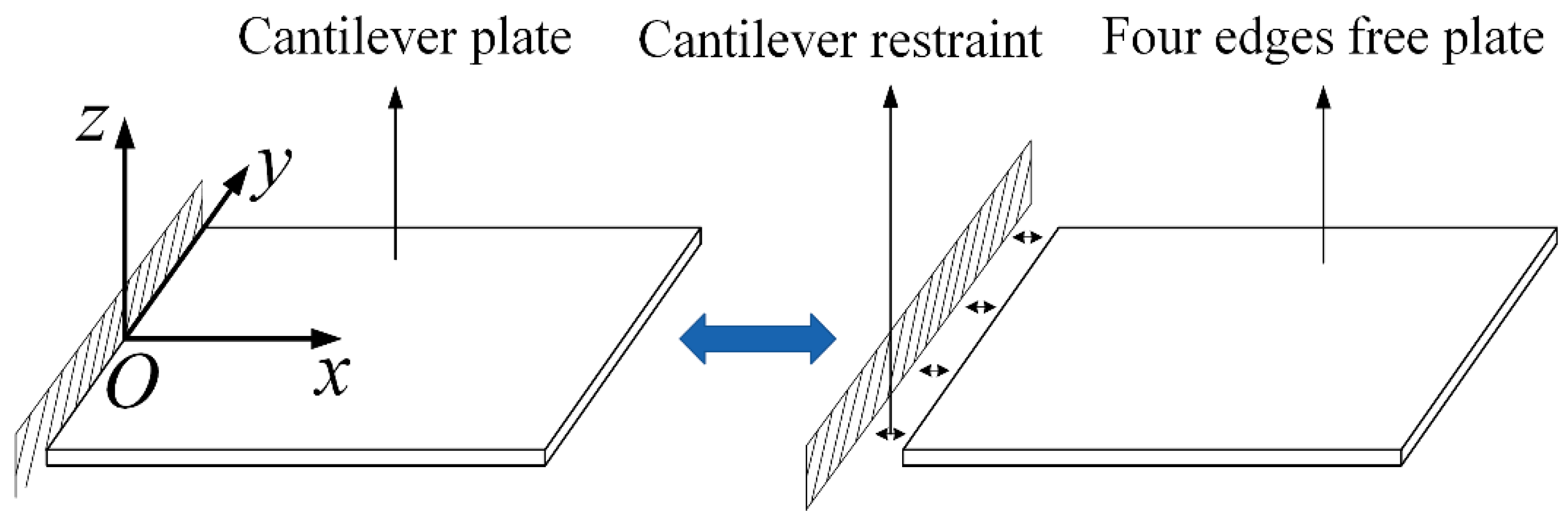
2.2. Constraining by Power Series Multiplier

The essence of a rectangular cantilever plate is that one of the ends is fully constrained. Inspired by the Lagrange multiplier method [22], the boundary condition of the cantilever plate can be described as the constraint expressed by the Lagrange multiplier applied on the free edge of the plate directly. Taking the edge in the y direction as the example, the constraint expression is given as

$$\mathsf{\Lambda }(y)={\displaystyle \sum _{i=j=0}^N{\lambda }_i{y}^j}={\lambda }_0+{\lambda }_{1}y+{\lambda }_2{y}^2+{\lambda }_3{y}^3+{\lambda }_4{y}^4+...,$$

(4)

where ${\lambda }_i$ is the Lagrange multiplier and acts as the coefficient of the polynomial. The number of terms N depends on the accuracy requirement.

Therefore, the cantilever plate can be established by applying the constraint on one edge of the four edges free plate as shown in Figure 1. As shown in Figure 2, the traditional Lagrange multiplier method [22] described point constraints. The power series multiplier method proposed in this paper describes the constraints in the interval.

The energy functional expression of the cantilever plate is

$$\prod =T_{\max }-U_{\max }+L_M,$$

(5)

where

$$\begin{array}{l}{T}_{\max }=\frac{1}{2}{\omega }^2\rho {\displaystyle {\int }_{-h}^h{\displaystyle {\int }_{-b}^b{\displaystyle {\int }_0^L{W}^2\mathrm{d}x\mathrm{d}y\mathrm{d}z}}},\\ U_{\max }=\frac{1}{2}{\displaystyle {\int }_{-h}^h{\displaystyle {\int }_{-b}^b{\displaystyle {\int }_0^L({\sigma }_x{\epsilon }_x+{\sigma }_y{\epsilon }_y+{\tau }_{xy}{\gamma }_{xy})\mathrm{d}x\mathrm{d}y\mathrm{d}z}}}.\end{array}$$

(6)

The symbol $\rho$ in T_max is the volume density of the plate. Symbols in U_max denote the stress–strain relationship as follows

$$\left[\begin{array}{l}{\sigma }_x\\ {\sigma }_y\\ {\tau }_{xy}\end{array}\right]=\left[\begin{array}{ccc}{Q}_{11}& Q_{12}& 0\\ Q_{21}& Q_{22}& 0\\ 0& 0& Q_{66}\end{array}\right]\left[\begin{array}{c}{\epsilon }_x\\ {\epsilon }_y\\ {\gamma }_{xy}\end{array}\right],\begin{array}{l}{Q}_{11}=Q_{22}=\frac{E}{1-{\mu }^2},\hfill \\ Q_{12}=\frac{E\mu }{1-{\mu }^2},Q_{66}=G,\hfill \end{array}$$

(7)

where E, G, and $\mu$ denote the elastic modulus, shear modulus, and Poisson ratio, respectively.

$L_M$ in Equation (5) is the term of the multiplier constraint. As the fixed boundary condition included the displacement and torsion angle, the expression of $L_M$ is given as follows

$$L_M={\displaystyle {\int }_{y_1}^{y_2}\left[{\displaystyle \sum _{i=j=0}^N{\lambda }_i{y}^{j}W(0,y)}+{\displaystyle \sum _{i=j=0}^N{\beta }_i{y}^j\frac{\partial W(0,y)}{\partial x}}\right]\mathrm{d}y},$$

(8)

where ${\lambda }_i$ and ${\beta }_i$ denote the constraining multipliers that corresponding to the displacement and rotating angle.

3. Dynamical Model of the Flexible Spacecraft with Solar Panels

In this section, the model of three-axis attitude stabilization spacecraft is established, which includes a central rigid-body platform and a pair of flexible solar panels.

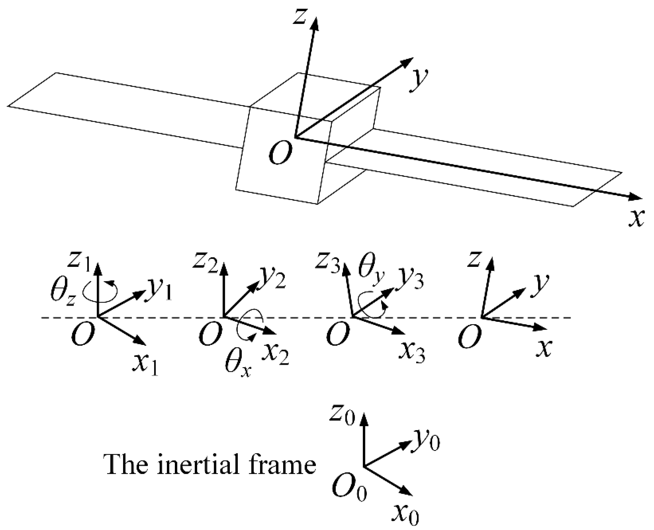
3.1. Geometric Description of the Model

To facilitate modeling, the flexible spacecraft can be modeled with a hub-plate system, as shown in Figure 3. The central rigid body is a cube structure. Point o is the center of the central rigid body. Coordinate system o₀ − x₀y₀z₀ is defined as the inertial frame. Coordinate system o − x₁y₁z₁ is defined as a coordinate system fixed on the central rigid body and parallel to the inertial frame. The coordinate frame o − xyz is defined as the companion coordinate system fixed on the central rigid body, which can be obtained by rotating o − x₁y₁z₁. As shown in Figure 3, o − x₁y₁z₁ first rotated θ_z around the z₁ axis then rotated θ_x around the x₂ axis. Finally, θ_y rotated around the y₃ axis to obtain o − xyz.

The transformation matrix of the coordinate system from o − xyz to o₀ − x₀y₀z₀ is expressed as follows

$$\mathbf{A}=\left[\begin{array}{ccc}\cos {\theta }_z& -\sin {\theta }_z& 0\\ \sin {\theta }_z& \cos {\theta }_z& 0\\ 0& 0& 1\end{array}\right]\left[\begin{array}{ccc}1& 0& 0\\ 0& \cos {\theta }_x& -\sin {\theta }_x\\ 0& \sin {\theta }_x& \cos {\theta }_x\end{array}\right]\left[\begin{array}{ccc}\cos {\theta }_y& 0& \sin {\theta }_y\\ 0& 1& 0\\ -\sin {\theta }_y& 0& \cos {\theta }_y\end{array}\right].$$

(9)

As the dynamical model is similar to that of Ref. [14], the total kinetic energy and strain energy has the same expression. By neglecting the same process of the derivation, the expressions of the kinetic and strain energy are given as follows

$$\begin{array}{ll}T=& \frac{1}{2}\rho {\displaystyle {\int }_{V_R}\{z^2{\left(\frac{\partial {\dot{w}}_1}{\partial x}\right)}^2+z^2{\left(\frac{\partial {\dot{w}}_1}{\partial y}\right)}^2+{\dot{w}}_1{}^2+{(x+r_0)}^2({\dot{\theta }}_z^2+{\dot{\theta }}_y^2)+y^2({\dot{\theta }}_x^2+{\dot{\theta }}_z^2)+z^2}\\ & \times ({\dot{\theta }}_{\mathrm{y}}^2+{\dot{\theta }}_x^2)+{\dot{x}}_o^2+{\dot{y}}_o^2+{\dot{z}}_o^2+2{\dot{z}}_o^2\left[{\dot{w}}_1-(x+r_0){\dot{\theta }}_y+y{\dot{\theta }}_x\right]+2(x+r_0){\dot{\theta }}_z{\dot{y}}_o\\ & -2y{\dot{\theta }}_z{\dot{x}}_o-2\left[(x+r_0){\dot{w}}_1+z^2\frac{\partial {\dot{w}}_1}{\partial x}\right]{\dot{\theta }}_y+2\left(y{\dot{w}}_1+z^2\frac{\partial {\dot{w}}_1}{\partial y}\right){\dot{\theta }}_x-2(x+r_0)y{\dot{\theta }}_x{\dot{\theta }}_y\}\mathrm{d}V\\ & +\frac{1}{2}\rho {\displaystyle {\int }_{V_L}{\Re }_T\mathrm{d}V}+\frac{1}{2}{m}_R({\dot{x}}_o^2+{\dot{y}}_o^2+{\dot{z}}_o^2)+\frac{1}{2}(J_z{\dot{\theta }}_z^2+J_x{\dot{\theta }}_x^2+J_y{\dot{\theta }}_y^2),\end{array}$$

(10)

$$\begin{array}{ll}U=& \frac{D}{2}{\displaystyle {\int }_0^L{\displaystyle {\int }_{-b}^b\left[{\left(\frac{{\partial }^2{w}_1}{\partial x^2}\right)}^2+2\mu \frac{{\partial }^2{w}_1}{\partial x^2}\frac{{\partial }^2{w}_1}{\partial y^2}+{\left(\frac{{\partial }^2{w}_1}{\partial y^2}\right)}^2+2(1-\mu ){\left(\frac{{\partial }^2{w}_1}{\partial x\partial y}\right)}^2\right]}\mathrm{d}x\mathrm{d}}y\\ & +\frac{D}{2}{\displaystyle {\int }_{-L}^0{\displaystyle {\int }_{-b}^b{\Re }_U\mathrm{d}x\mathrm{d}y}.}\end{array}$$

(11)

where x, y, and z are the coordinates of any point in the random coordinate system o − xyz. w₁ is the displacement of any point on the solar panel along the z axis. r₀ is half the length of the sides of the central rigid body (cube). x_o, y_o, and z_o are the displacements of the central rigid body. θ_x, θ_y, and θz are the corners of the central rigid body. m_R is the mass of the central rigid body. J_x, J_y, and J_z are the moment of inertia of the central rigid body. Replacing r₀ and w₁ in the first integral of Equation (10) with -r₀ and w₂ yields ${\Re }_T$ in this equation. Similarly, replacing w₁ in the first integral expression of Equation (11) with w₂ leads to ${\Re }_U$ in this equation. It should be noted that in kinetic energy Expression (10), nonlinear coupling terms of degree three and higher are ignored, which are products of w₁, w₂, θ_x, θ_y, θ_z, x_o, y_o, and z_o and their derivatives with respect to time t and coordinates x and y such as ${\dot{\theta }}_1{\dot{\theta }}_3\partial w/\partial x$.

In Equation (11), D is the flexural stiffness of the solar panel, where L and b are one half of the length and width of the solar panel, respectively. The expression of flexural stiffness D is

$$D=\frac{2E{h}^3}{3(1-{\mu }^2)}.$$

(12)

3.2. Characteristic Equation of the Spacecraft

As solar panels are fixed on the spacecraft, each solar panel can be regarded as a cantilever plate. According to the construction method of the cantilever plate mentioned in Section 2.2, the energy functional of the spacecraft can be constructed as follows

$$\begin{array}{ll}\prod =& U_{\max }-T_{\max }+{\displaystyle {\int }_{-b}^b{\displaystyle \sum _{i=j=0}^N{\lambda }_{R_i}{y}^j\cdot W_R(0,y)\mathrm{d}y}}+{\displaystyle {\int }_{-b}^b{\displaystyle \sum _{i=j=0}^N{\beta }_{R_i}{y}^j\cdot \frac{\partial W_R(0,y)}{\partial x}\mathrm{d}y}}\\ & +{\displaystyle {\int }_{-b}^b{\displaystyle \sum _{i=j=0}^N{\lambda }_{L_i}{y}^j\cdot W_L(0,y)\mathrm{d}y}}+{\displaystyle {\int }_{-b}^b{\displaystyle \sum _{i=j=0}^N{\beta }_{L_i}{y}^j\cdot \frac{\partial W_L(0,y)}{\partial x}\mathrm{d}y}}.\end{array}$$

(13)

According to the concept of rigid-flexible coupled modes in Ref. [14], the rigid body motion of the spacecraft can be expressed as the product of a constant and a time term

$$q_o=S_o\sin \omega t,{\theta }_q={\theta }_0^{(q)}\sin \omega t,q=x,y,z,S=X,Y,Z,$$

(14)

where $S_o$ and ${\theta }_0^{(q)}$ are unknown coefficients.

The solar panel vibration displacement Expression (1) and the spacecraft rigid body displacement Expression (14) are substituted into the flexible spacecraft kinetic energy Expression (10) and potential energy Expression (11). Through the Rayleigh–Ritz method, the system Rayleigh quotient with respect to the coefficients $X_o$, $Y_o$, $Z_o$, ${\theta }_0^{(x)}$, ${\theta }_0^{(y)}$, ${\theta }_0^{(z)}$, $A_{mn}^{(1)}$, $A_{mn}^{(2)}$, ${\lambda }_{R_i}$, ${\beta }_{R_i}$, ${\lambda }_{L_i}$, and ${\beta }_{L_i}$ is minimized

$$\frac{\partial \prod }{\partial X_o}=0,\frac{\partial \prod }{\partial Y_o}=0,\frac{\partial \prod }{\partial Z_o}=0,$$

(15)

$$\frac{\partial \prod }{\partial {\theta }_0^{(x)}}=0,\frac{\partial \prod }{\partial {\theta }_0^{(y)}}=0,\frac{\partial \prod }{\partial {\theta }_0^{(z)}}=0,$$

(16)

$$\frac{\partial \prod }{\partial A_{mn}^{(i)}}=0,i=1,2,$$

(17)

$$\frac{\partial \prod }{\partial {\lambda }_{R_i}}=0,\frac{\partial \prod }{\partial {\beta }_{R_i}}=0,\frac{\partial \prod }{\partial {\lambda }_{L_i}}=0,\frac{\partial \prod }{\partial {\beta }_{L_i}}=0,i=0,1,\dots ,N.$$

(18)

The characteristic equation of the flexible spacecraft equipped with a pair of solar panels is obtained as follows

$$(\mathbf{K}-{\omega }^2\mathbf{M}+\mathsf{\Lambda })\mathbf{X}=\mathbf{0},$$

(19)

where X is a column vector containing all unknown coefficients in the following form

$$\begin{array}{c}\mathbf{X}=[X_o,Y_o,Z_o,{\theta }_0^{(x)},{\theta }_0^{(y)},{\theta }_0^{(z)},A_{11}^{(1)},A_{12}^{(1)},\dots ,A_{m_t{n}_t}^{(1)},A_{11}^{(2)},A_{12}^{(2)},\dots ,A_{m_t{n}_t}^{(2)},\\ {\lambda }_{R_0},\dots ,{\lambda }_{R_N},{\beta }_{R_0},\dots ,{\beta }_{R_N},{\lambda }_{L_0},\dots ,{\lambda }_{L_N},{\beta }_{L_0},\dots ,{\beta }_{L_N}{]}^{\mathrm{T}}.\end{array}$$

(20)

K is the matrix of $[6+2m_t{n}_t+4(N+1)]\times [6+2m_t{n}_t+4(N+1)]$

$$\mathbf{K}=\left[\begin{array}{cccc}{\mathbf{0}}_{6\times 6}& {\mathbf{0}}_{6\times m_t{n}_t}& {\mathbf{0}}_{6\times m_t{n}_t}& {\mathbf{0}}_{6\times 4(N+1)}\\ {\mathbf{0}}_{m_t{n}_t\times 6}& {\mathbf{K}}_{77}& {\mathbf{0}}_{m_t{n}_t\times m_t{n}_t}& {\mathbf{0}}_{m_t{n}_t\times 4(N+1)}\\ {\mathbf{0}}_{m_t{n}_t\times 6}& {\mathbf{0}}_{m_t{n}_t\times m_t{n}_t}& {\mathbf{K}}_{88}& {\mathbf{0}}_{m_t{n}_t\times 4(N+1)}\\ {\mathbf{0}}_{4(N+1)\times 6}& {\mathbf{0}}_{4(N+1)\times m_t{n}_t}& {\mathbf{0}}_{4(N+1)\times m_t{n}_t}& {\mathbf{0}}_{4(N+1)\times 4(N+1)}\end{array}\right],$$

(21)

where K₇₇ and K₈₈ are the block matrices of K. Their size is $m_t{n}_t\times m_t{n}_t$. The elements of the two are denoted as

$$\begin{array}{ll}{({\mathbf{K}}_{77})}_{m_i{n}_i,m_j{n}_j}=& D{\displaystyle {\int }_0^L{\displaystyle {\int }_{-b}^b[\frac{{\partial }^2{\phi }_{m_i}^{(1)}(x)}{\partial x^2}{\phi }_{n_i}^{(1)}(y)\frac{{\partial }^2{\phi }_{m_j}^{(1)}(x)}{\partial x^2}{\phi }_{n_j}^{(1)}(y)}}\\ & +\mu {\phi }_{m_i}^{(1)}(x)\frac{{\partial }^2{\phi }_{n_i}^{(1)}(y)}{\partial y^2}\frac{{\partial }^2{\phi }_{m_j}^{(1)}(x)}{\partial x^2}{\phi }_{n_j}^{(1)}(y)\\ & +\mu \frac{{\partial }^2{\phi }_{m_i}^{(1)}(x)}{\partial x^2}{\phi }_{n_i}^{(1)}(y){\phi }_{m_j}^{(1)}(x)\frac{{\partial }^2{\phi }_{n_j}^{(1)}(y)}{\partial y^2}\\ & +{\phi }_{m_i}^{(1)}(x)\frac{{\partial }^2{\phi }_{n_i}^{(1)}(y)}{\partial y^2}{\phi }_{m_j}^{(1)}(x)\frac{{\partial }^2{\phi }_{n_j}^{(1)}(y)}{\partial y^2}\\ & +2(1-\mu )\frac{\partial {\phi }_{m_i}^{(1)}(x)}{\partial x}\frac{\partial {\phi }_{n_i}^{(1)}(y)}{\partial y}\frac{\partial {\phi }_{m_j}^{(1)}(x)}{\partial x}\frac{\partial {\phi }_{n_j}^{(1)}(y)}{\partial y}]\mathrm{d}y\mathrm{d}x,\end{array}$$

(22)

$$\begin{array}{ll}{({\mathbf{K}}_{88})}_{m_i{n}_i,m_j{n}_j}=& D{\displaystyle {\int }_{-L}^0{\displaystyle {\int }_{-b}^b[\frac{{\partial }^2{\phi }_{m_i}^{(2)}(x)}{\partial x^2}{\phi }_{n_i}^{(2)}(y)\frac{{\partial }^2{\phi }_{m_j}^{(2)}(x)}{\partial x^2}{\phi }_{n_j}^{(2)}(y)}}\\ & +\mu {\phi }_{m_i}^{(2)}(x)\frac{{\partial }^2{\phi }_{n_i}^{(2)}(y)}{\partial y^2}\frac{{\partial }^2{\phi }_{m_j}^{(2)}(x)}{\partial x^2}{\phi }_{n_j}^{(2)}(y)\\ & +\mu \frac{{\partial }^2{\phi }_{m_i}^{(2)}(x)}{\partial x^2}{\phi }_{n_i}^{(2)}(y){\phi }_{m_j}^{(2)}(x)\frac{{\partial }^2{\phi }_{n_j}^{(2)}(y)}{\partial y^2}\\ & +{\phi }_{m_i}^{(2)}(x)\frac{{\partial }^2{\phi }_{n_i}^{(2)}(y)}{\partial y^2}{\phi }_{m_j}^{(2)}(x)\frac{{\partial }^2{\phi }_{n_j}^{(2)}(y)}{\partial y^2}\\ & +2(1-\mu )\frac{\partial {\phi }_{m_i}^{(2)}(x)}{\partial x}\frac{\partial {\phi }_{n_i}^{(2)}(y)}{\partial y}\frac{\partial {\phi }_{m_j}^{(2)}(x)}{\partial x}\frac{\partial {\phi }_{n_j}^{(2)}(y)}{\partial y}]\mathrm{d}y\mathrm{d}x,\end{array}$$

(23)

where $m_i,m_j=1,2,\dots ,m_t$ and $n_i,n_j=1,2,\dots ,n_t$.

M is the matrix of $[6+2m_t{n}_t+4(N+1)]\times [6+2m_t{n}_t+4(N+1)]$

$$\mathbf{M}=\left[\begin{array}{cc}{\mathbf{M}}_s& {\mathbf{0}}_{(6+2m_t{n}_t)\times 4(N+1)}\\ {\mathbf{0}}_{4(N+1)\times (2m_t{n}_t+6)}& {\mathbf{0}}_{4(N+1)\times 4(N+1)}\end{array}\right],$$

(24)

where

$${\mathbf{M}}_s=\left[\begin{array}{cccccccc}{M}_{11}& 0& 0& 0& 0& M_{16}& {\mathbf{0}}_{1\times m_t{n}_t}& {\mathbf{0}}_{1\times m_t{n}_t}\\ 0& M_{22}& 0& 0& 0& M_{26}& {\mathbf{0}}_{1\times m_t{n}_t}& {\mathbf{0}}_{1\times m_t{n}_t}\\ 0& 0& M_{33}& M_{34}& M_{35}& 0& {\mathbf{M}}_{37}& {\mathbf{M}}_{38}\\ 0& 0& M_{43}& M_{44}& 0& 0& {\mathbf{M}}_{47}& {\mathbf{M}}_{48}\\ 0& 0& M_{53}& 0& M_{55}& 0& {\mathbf{M}}_{57}& {\mathbf{M}}_{58}\\ M_{61}& M_{62}& 0& 0& 0& M_{66}& {\mathbf{0}}_{1\times m_t{n}_t}& {\mathbf{0}}_{1\times m_t{n}_t}\\ {\mathbf{0}}_{m_t{n}_t\times 1}& {\mathbf{0}}_{m_t{n}_t\times 1}& {\mathbf{M}}_{73}& {\mathbf{M}}_{74}& {\mathbf{M}}_{75}& {\mathbf{0}}_{m_t{n}_t\times 1}& {\mathbf{M}}_{77}& {\mathbf{0}}_{m_t{n}_t\times m_t{n}_t}\\ {\mathbf{0}}_{m_t{n}_t\times 1}& {\mathbf{0}}_{m_t{n}_t\times 1}& {\mathbf{M}}_{83}& {\mathbf{M}}_{84}& {\mathbf{M}}_{85}& {\mathbf{0}}_{m_t{n}_t\times 1}& {\mathbf{0}}_{m_t{n}_t\times m_t{n}_t}& {\mathbf{M}}_{88}\end{array}\right],$$

(25)

where

$$\begin{array}{l}{M}_{11}=\rho {\displaystyle {\int }_0^L{\displaystyle {\int }_{-b}^{b}2h\mathrm{d}y}}\mathrm{d}x+\rho {\displaystyle {\int }_{-L}^0{\displaystyle {\int }_{-b}^{b}2h\mathrm{d}y}}\mathrm{d}x+m_R,M_{22}=M_{11},M_{33}=M_{11},\\ M_{16}=\rho {\displaystyle {\int }_0^L{\displaystyle {\int }_{-b}^b-2hy\mathrm{d}y}}\mathrm{d}x+\rho {\displaystyle {\int }_{-L}^0{\displaystyle {\int }_{-b}^b-2hy\mathrm{d}y}}\mathrm{d}x,M_{61}=M_{16},\\ M_{26}=\rho {\displaystyle {\int }_0^L{\displaystyle {\int }_{-b}^{b}2h(x+r_0)\mathrm{d}y}}\mathrm{d}x+\rho {\displaystyle {\int }_{-L}^0{\displaystyle {\int }_{-b}^{b}2h(x-r_0)\mathrm{d}y}}\mathrm{d}x,M_{62}=M_{26},\\ M_{34}=-M_{16},M_{35}=-M_{26},M_{43}=M_{34},M_{53}=M_{35},\\ M_{44}=\rho {\displaystyle {\int }_0^L{\displaystyle {\int }_{-b}^b\left(2h{y}^2+\frac{2}{3}{h}^3\right)\mathrm{d}y}}\mathrm{d}x+\rho {\displaystyle {\int }_{-L}^0{\displaystyle {\int }_{-b}^b\left(2h{y}^2+\frac{2}{3}{h}^3\right)\mathrm{d}y}}\mathrm{d}x+J_x,\\ M_{55}=\rho {\displaystyle {\int }_0^L{\displaystyle {\int }_{-b}^b\left[2h{(x+r_0)}^2+\frac{2}{3}{h}^3\right]\mathrm{d}y}}\mathrm{d}x+\rho {\displaystyle {\int }_{-L}^0{\displaystyle {\int }_{-b}^b\left[2h{(x-r_0)}^2+\frac{2}{3}{h}^3\right]\mathrm{d}y}}\mathrm{d}x+J_y,\\ M_{66}=\rho {\displaystyle {\int }_0^L{\displaystyle {\int }_{-b}^b\left[2h{(x+r_0)}^2+2h{y}^2\right]\mathrm{d}y}}\mathrm{d}x+\rho {\displaystyle {\int }_{-L}^0{\displaystyle {\int }_{-b}^b\left[2h{(x-r_0)}^2+2h{y}^2\right]\mathrm{d}y}}\mathrm{d}x+J_z.\end{array}$$

(26)

${\mathbf{M}}_{37}$, ${\mathbf{M}}_{38}$, ${\mathbf{M}}_{47}$, ${\mathbf{M}}_{48}$, ${\mathbf{M}}_{57}$ and ${\mathbf{M}}_{58}$ are $1\times m_t{n}_t$ row vectors. Its elements are

$$\begin{array}{l}{({\mathbf{M}}_{37})}_{m_i{n}_i}=\rho {\displaystyle {\int }_0^L{\displaystyle {\int }_{-b}^{b}2h{\phi }_{m_i}^{(1)}(x){\phi }_{n_i}^{(1)}(y)\mathrm{d}y}}\mathrm{d}x,\\ {({\mathbf{M}}_{38})}_{m_i{n}_i}=\rho {\displaystyle {\int }_{-L}^0{\displaystyle {\int }_{-b}^{b}2h{\phi }_{m_i}^{(2)}(x){\phi }_{n_i}^{(2)}(y)\mathrm{d}y}}\mathrm{d}x,\\ {({\mathbf{M}}_{47})}_{m_i{n}_i}=\rho {\displaystyle {\int }_0^L{\displaystyle {\int }_{-b}^b\left[2hy{\phi }_{m_i}^{(1)}(x){\phi }_{n_i}^{(1)}(y)+\frac{2}{3}{h}^3{\phi }_{m_i}^{(1)}(x)\frac{\partial {\phi }_{n_i}^{(1)}(y)}{\partial y}\right]\mathrm{d}y}}\mathrm{d}x,\\ {({\mathbf{M}}_{48})}_{m_i{n}_i}=\rho {\displaystyle {\int }_{-L}^0{\displaystyle {\int }_{-b}^b\left[2hy{\phi }_{m_i}^{(2)}(x){\phi }_{n_i}^{(2)}(y)+\frac{2}{3}{h}^3{\phi }_{m_i}^{(2)}(x)\frac{\partial {\phi }_{n_i}^{(2)}(y)}{\partial y}\right]\mathrm{d}y}}\mathrm{d}x,\\ {({\mathbf{M}}_{57})}_{m_i{n}_i}=\rho {\displaystyle {\int }_0^L{\displaystyle {\int }_{-b}^b\left[-2h(x+r_0){\phi }_{m_i}^{(1)}(x){\phi }_{n_i}^{(1)}(y)-\frac{2}{3}{h}^3\frac{\partial {\phi }_{m_i}^{(1)}(x)}{\partial x}{\phi }_{n_i}^{(1)}(y)\right]\mathrm{d}y}}\mathrm{d}x,\\ {({\mathbf{M}}_{58})}_{m_i{n}_i}=\rho {\displaystyle {\int }_{-L}^0{\displaystyle {\int }_{-b}^b\left[-2h(x-r_0){\phi }_{m_i}^{(2)}(x){\phi }_{n_i}^{(2)}(y)-\frac{2}{3}{h}^3\frac{\partial {\phi }_{m_i}^{(2)}(x)}{\partial x}{\phi }_{n_i}^{(2)}(y)\right]\mathrm{d}y}}\mathrm{d}x,\end{array}$$

(27)

${\mathbf{M}}_{73}$, ${\mathbf{M}}_{83}$, ${\mathbf{M}}_{74}$, ${\mathbf{M}}_{84}$, ${\mathbf{M}}_{75}$ and ${\mathbf{M}}_{85}$ are $m_t{n}_t\times 1$ column vectors. Its elements are

$$\begin{array}{l}{\mathbf{M}}_{73}={\mathbf{M}}_{37}^{\mathrm{T}},{\mathbf{M}}_{74}={\mathbf{M}}_{47}^{\mathrm{T}},{\mathbf{M}}_{75}={\mathbf{M}}_{57}^{\mathrm{T}},\\ {\mathbf{M}}_{83}={\mathbf{M}}_{38}^{\mathrm{T}},{\mathbf{M}}_{84}={\mathbf{M}}_{48}^{\mathrm{T}},{\mathbf{M}}_{85}={\mathbf{M}}_{58}^{\mathrm{T}}.\end{array}$$

(28)

M₇₇ and M₈₈ are the block matrices of M. Their size is $m_t{n}_t\times m_t{n}_t$. The elements of the two are denoted as

$$\begin{array}{ll}{({\mathbf{M}}_{77})}_{m_i{n}_i,m_j{n}_j}=& \rho {\displaystyle {\int }_0^L{\displaystyle {\int }_{-b}^b[\frac{2}{3}{h}^3\frac{\partial {\phi }_{m_i}^{(1)}(x)}{\partial x}{\phi }_{n_i}^{(1)}(y)\frac{\partial {\phi }_{m_j}^{(1)}(x)}{\partial x}{\phi }_{n_j}^{(1)}(y)}}\\ & +\frac{2}{3}{h}^3{\phi }_{m_i}^{(1)}(x)\frac{\partial {\phi }_{n_i}^{(1)}(y)}{\partial y}{\phi }_{m_j}^{(1)}(x)\frac{\partial {\phi }_{n_j}^{(1)}(y)}{\partial y}\\ & +2h{\phi }_{m_i}^{(1)}(x){\phi }_{n_i}^{(1)}(y){\phi }_{m_j}^{(1)}(x){\phi }_{n_j}^{(1)}(y)]\mathrm{d}y\mathrm{d}x,\end{array}$$

(29)

$$\begin{array}{ll}{({\mathbf{M}}_{88})}_{m_i{n}_i,m_j{n}_j}=& \rho {\displaystyle {\int }_{-L}^0{\displaystyle {\int }_{-b}^b[\frac{2}{3}{h}^3\frac{\partial {\phi }_{m_i}^{(2)}(x)}{\partial x}{\phi }_{n_i}^{(2)}(y)\frac{\partial {\phi }_{m_j}^{(2)}(x)}{\partial x}{\phi }_{n_j}^{(2)}(y)}}\\ & +\frac{2}{3}{h}^3{\phi }_{m_i}^{(2)}(x)\frac{\partial {\phi }_{n_i}^{(2)}(y)}{\partial y}{\phi }_{m_j}^{(2)}(x)\frac{\partial {\phi }_{n_j}^{(2)}(y)}{\partial y}\\ & +2h{\phi }_{m_i}^{(2)}(x){\phi }_{n_i}^{(2)}(y){\phi }_{m_j}^{(2)}(x){\phi }_{n_j}^{(2)}(y)]\mathrm{d}y\mathrm{d}x,\end{array}$$

(30)

$\mathsf{\Lambda }$ is the matrix of $[6+2m_t{n}_t+4(N+1)]\times [6+2m_t{n}_t+4(N+1)]$

$$\mathsf{\Lambda }=\left[\begin{array}{ccc}{\mathbf{0}}_{6\times 6}& {\mathbf{0}}_{6\times 2m_t{n}_t}& {\mathbf{0}}_{6\times 4(N+1)}\\ {\mathbf{0}}_{2m_t{n}_t\times 6}& {\mathbf{0}}_{2m_t{n}_t\times 2m_t{n}_t}& {\mathsf{\Lambda }}_{23}\\ {\mathbf{0}}_{4(N+1)\times 6}& {\mathsf{\Lambda }}_{32}& {\mathbf{0}}_{4(N+1)\times 4(N+1)}\end{array}\right],$$

(31)

${\mathsf{\Lambda }}_{23}$ is the block matrix of $\mathsf{\Lambda }$. Its size is $2m_t{n}_t\times 4(N+1)$. It said for

$${\mathsf{\Lambda }}_{23}=\left[\begin{array}{cc}{\mathsf{\Lambda }}_{{23}_R}& {\mathbf{0}}_{m_t{n}_t\times 2(N+1)}\\ {\mathbf{0}}_{m_t{n}_t\times 2(N+1)}& {\mathsf{\Lambda }}_{{23}_L}\end{array}\right],$$

(32)

${\mathsf{\Lambda }}_{32}$ is the block matrix of $\mathsf{\Lambda }$. Its size is $4(N+1)\times 2m_t{n}_t$. It said for

$${\mathsf{\Lambda }}_{32}={\mathsf{\Lambda }}_{23}^{\mathrm{T}},$$

(33)

where ${\mathsf{\Lambda }}_{{23}_R}$ and ${\mathsf{\Lambda }}_{{23}_L}$ are the block matrices of ${\mathsf{\Lambda }}_{23}$. Their size is $m_t{n}_t\times 2(N+1)$. The elements of the two are denoted as

$${\mathsf{\Lambda }}_{{23}_R}=\left[{\mathsf{\lambda }}_R,{\mathsf{\beta }}_R\right],{\mathsf{\Lambda }}_{{23}_L}=\left[{\mathsf{\lambda }}_L,{\mathsf{\beta }}_L\right],$$

(34)

where ${\mathsf{\lambda }}_R$ and ${\mathsf{\beta }}_R$ are the block matrices of ${\mathsf{\Lambda }}_{{23}_R}$, ${\mathsf{\lambda }}_L$ and ${\mathsf{\beta }}_L$ are the block matrices of ${\mathsf{\Lambda }}_{{23}_L}$. Their size is $m_t{n}_t\times (N+1)$. Their elements are denoted as

$${\mathsf{\lambda }}_R=\left[\begin{array}{ccc}{\displaystyle {\int }_{-b}^b{\phi }_1^{(1)}(0){\phi }_1^{(1)}(y)\mathrm{d}y}& \cdots & {\displaystyle {\int }_{-b}^b{y}^{(N)}{\phi }_1^{(1)}(0){\phi }_1^{(1)}(y)\mathrm{d}y}\\ {\displaystyle {\int }_{-b}^b{\phi }_1^{(1)}(0){\phi }_2^{(1)}(y)\mathrm{d}y}& \cdots & {\displaystyle {\int }_{-b}^b{y}^{(N)}{\phi }_1^{(1)}(0){\phi }_2^{(1)}(y)\mathrm{d}y}\\ ⋮& \ddots & ⋮\\ {\displaystyle {\int }_{-b}^b{\phi }_{m_t}^{(1)}(0){\phi }_{n_t}^{(1)}(y)\mathrm{d}y}& \cdots & {\displaystyle {\int }_{-b}^b{y}^{(N)}{\phi }_{m_t}^{(1)}(0){\phi }_{n_t}^{(1)}(y)\mathrm{d}y}\end{array}\right],$$

(35)

$${\mathsf{\beta }}_R=\left[\begin{array}{ccc}{\displaystyle {\int }_{-b}^b\frac{\partial {\phi }_1^{(1)}(0)}{\partial x}{\phi }_1^{(1)}(y)\mathrm{d}y}& \cdots & {\displaystyle {\int }_{-b}^b{y}^{(N)}\frac{\partial {\phi }_1^{(1)}(0)}{\partial x}{\phi }_1^{(1)}(y)\mathrm{d}y}\\ {\displaystyle {\int }_{-b}^b\frac{\partial {\phi }_1^{(1)}(0)}{\partial x}{\phi }_2^{(1)}(y)\mathrm{d}y}& \cdots & {\displaystyle {\int }_{-b}^b{y}^{(N)}\frac{\partial {\phi }_1^{(1)}(0)}{\partial x}{\phi }_2^{(1)}(y)\mathrm{d}y}\\ ⋮& \ddots & ⋮\\ {\displaystyle {\int }_{-b}^b\frac{\partial {\phi }_{m_t}^{(1)}(0)}{\partial x}{\phi }_{n_t}^{(1)}(y)\mathrm{d}y}& \cdots & {\displaystyle {\int }_{-b}^b{y}^{(N)}\frac{\partial {\phi }_{m_t}^{(1)}(0)}{\partial x}{\phi }_{n_t}^{(1)}(y)\mathrm{d}y}\end{array}\right],$$

(36)

$${\mathsf{\lambda }}_L=\left[\begin{array}{ccc}{\displaystyle {\int }_{-b}^b{\phi }_1^{(2)}(0){\phi }_1^{(2)}(y)\mathrm{d}y}& \cdots & {\displaystyle {\int }_{-b}^b{y}^{(N)}{\phi }_1^{(2)}(0){\phi }_1^{(2)}(y)\mathrm{d}y}\\ {\displaystyle {\int }_{-b}^b{\phi }_1^{(2)}(0){\phi }_2^{(2)}(y)\mathrm{d}y}& \cdots & {\displaystyle {\int }_{-b}^b{y}^{(N)}{\phi }_1^{(2)}(0){\phi }_2^{(2)}(y)\mathrm{d}y}\\ ⋮& \ddots & ⋮\\ {\displaystyle {\int }_{-b}^b{\phi }_{m_t}^{(2)}(0){\phi }_{n_t}^{(2)}(y)\mathrm{d}y}& \cdots & {\displaystyle {\int }_{-b}^b{y}^{(N)}{\phi }_{m_t}^{(2)}(0){\phi }_{n_t}^{(2)}(y)\mathrm{d}y}\end{array}\right],$$

(37)

$${\mathsf{\beta }}_L=\left[\begin{array}{ccc}{\displaystyle {\int }_{-b}^b\frac{\partial {\phi }_1^{(2)}(0)}{\partial x}{\phi }_1^{(2)}(y)\mathrm{d}y}& \cdots & {\displaystyle {\int }_{-b}^b{y}^{(N)}\frac{\partial {\phi }_1^{(2)}(0)}{\partial x}{\phi }_1^{(2)}(y)\mathrm{d}y}\\ {\displaystyle {\int }_{-b}^b\frac{\partial {\phi }_1^{(2)}(0)}{\partial x}{\phi }_2^{(2)}(y)\mathrm{d}y}& \cdots & {\displaystyle {\int }_{-b}^b{y}^{(N)}\frac{\partial {\phi }_1^{(2)}(0)}{\partial x}{\phi }_2^{(2)}(y)\mathrm{d}y}\\ ⋮& \ddots & ⋮\\ {\displaystyle {\int }_{-b}^b\frac{\partial {\phi }_{m_t}^{(2)}(0)}{\partial x}{\phi }_{n_t}^{(2)}(y)\mathrm{d}y}& \cdots & {\displaystyle {\int }_{-b}^b{y}^{(N)}\frac{\partial {\phi }_{m_t}^{(2)}(0)}{\partial x}{\phi }_{n_t}^{(2)}(y)\mathrm{d}y}\end{array}\right],$$

(38)

Frequencies and mode shapes of the flexible spacecraft can be obtained by solving the characteristic Equation (19). The first six of these frequencies are zero and correspond to rigid body translations (x_o, y_o, and z_o) and attitude motions (θ_x, θ_y, and θ_z) of the whole flexible spacecraft. In such a situation, the solar panel does not deform. Therefore, these six frequencies were ignored in the following analysis.

4. Numerical Simulation and Discussion

4.1. Validity Verification and Convergence Analysis of the Method

In order to verify the effectiveness and convergence of the power series multiplier constraint method proposed in this paper, the four-sided free plate is equivalent to the cantilever plate and the natural characteristic is obtained by using this method. At the same time, the natural frequency of the cantilever plate is obtained by using the finite element software ANSYS, which is presented as the reference. The length L of the four-sided free plate studied in this paper is 2 m, 4 m, and 8 m. The width 2b is 2 m, 4 m, and 8 m. The thickness 2h is 0.02 m. The material of the plate is aluminum alloy. The elastic modulus E is 6.89 × 10¹⁰. The mass density ρ is 2.8 × 10³. Poisson ratio μ is 0.33.

To facilitate the convergence analysis, the relative error R_t is defined as

$$R_t=\frac{f_{m_t{n}_t}-f_{\mathrm{fem}}}{f_{\mathrm{fem}}}\times 100\%,$$

(39)

where $f_{m_t{n}_t}$ represents the frequency calculation value when m_t and n_t are taken by orthogonal polynomials in x and y directions. $f_{\mathrm{fem}}$ is the frequency calculation value of finite element software ANSYS.

As shown in Figure 4, the convergence of the 1st, 2nd, 3rd, and 4th order frequencies of the cantilever plate are given, where m_t and n_t are from 4 to 11, respectively. The cantilever plate is established by the four-side free plate constrained by the power series multiplier constraint method. According to the figure, in this m_t = 4, the relative error R_t does not change much with the increase of n_t value. The relative error R_t of the 1st order frequency is reduced from 1.5% to 0.4%, but always within 2%. The relative errors R_t of the 2nd, 3rd and 4th order frequencies are all greater than 2%. In this n_t = 4, the relative error R_t decreased significantly as the value of m_t increases. The relative error R_t of the 1st order frequency is within 1%. In this m_t = n_t = 5, the relative error R_t is already within 1%. In this m_t = n_t = 11, the relative error R_t is also within 1% and tends to zero. The relative error R_t of the 1st, 2nd, 3rd, and 4th order frequencies of the cantilever plate has a similar trend with the increase of m_t and n_t values. First, it decreases rapidly and then gradually goes to zero. This shows that the power series multiplier constraint method has excellent convergence. As can be seen from the figure, in this m_t = 11 and n_t = 7, each order frequency of the plate can be obtained with sufficient accuracy.

As can be seen from

Table 1. The first eight order frequencies of plates with different widths f (Hz) (L = 8 m, m_t = 11, n_t = 7, N = 2).

Order	2b = 2 m			2b = 4 m			2b = 8 m
	ANSYS	Method	Rt (%)	ANSYS	Method	Rt (%)	ANSYS	Method	Rt (%)
1	0.255	0.255	0.00	0.258	0.257	−0.39	0.261	0.259	−0.77
2	1.595	1.593	−0.13	1.095	1.095	0.00	0.631	0.630	−0.16
3	2.031	2.033	0.10	1.607	1.604	−0.19	1.593	1.590	−0.19
4	4.482	4.476	−0.13	3.575	3.573	−0.06	2.043	2.041	−0.10
5	6.278	6.283	0.08	4.511	4.505	−0.13	2.307	2.305	−0.09
6	8.825	8.814	−0.12	6.890	6.888	−0.03	4.041	4.038	−0.07
7	11.051	11.057	0.05	6.997	6.995	−0.03	4.613	4.609	−0.09
8	14.647	14.719	0.49	8.890	8.881	−0.10	4.803	4.712	−1.89

, the length L of the cantilever plate is 8 m, and the relative error R_t of the 1st and 3rd order frequencies kept increasing as the width 2b of the plate increased. The relative error R_t of 2nd, 4th, 6th, 7th, and 8th order frequencies decrease first and increase then. The relative error of the 5th order frequency R_t increases first and then decreases. The relative errors R_t of the first eight order frequencies are kept within 2%. This shows that the result of calculating the type $L\ge 2b$ by the method in this paper is reasonable.

As can be seen from

Table 2. The first eight order frequencies of plates with different lengths f (Hz) (2b = 4 m, m_t = 11, n_t = 7, N = 2).

Order	L = 2 m			L = 4 m			L = 8 m
	ANSYS	Method	Rt (%)	ANSYS	Method	Rt (%)	ANSYS	Method	Rt (%)
1	4.210	4.175	−0.83	1.044	1.038	−0.57	0.258	0.257	−0.39
2	6.376	6.358	−0.28	2.525	2.521	−0.16	1.095	1.095	0.00
3	12.118	12.097	−0.17	6.371	6.360	−0.17	1.607	1.604	−0.19
4	22.763	18.725	−17.74	8.170	8.164	−0.07	3.575	3.573	−0.06
5	26.326	26.280	−0.17	9.228	9.220	−0.09	4.511	4.505	−0.13
6	29.665	28.881	−2.64	16.161	16.153	−0.05	6.890	6.888	−0.03
7	37.529	32.080	−14.52	18.461	18.434	−0.15	6.997	6.995	−0.03
8	40.944	37.572	−8.24	19.219	18.847	−1.94	8.890	8.881	−0.10

, when the width 2b of the cantilever plate is 4 m, the relative error R_t of the 1st, 2nd, 4th, 6th, 7th, and 8th order frequencies kept decreasing as the length L of the plate increases. The relative error R_t of the 3rd order frequency is a small increase. The relative error R_t of the 5th order frequency decreases and then increases. In this the length L of the plate is 4 m and 8 m, the relative error R_t of the first eight order frequencies is kept within 2%. This again shows the result of calculating type $L\ge 2b$ by the method in this paper is reasonable. However, in this the length L of the plate is 2 m, the relative errors R_t of the 4th, 6th, 7th, and 8th order frequencies are all greater than 2%. The relative error R_t of the 4th frequency reached 17.74%. This indicates that the result of calculating the type $2b>L$ by the power series multiplier constraint method is not accurate.

Table 3. The first eight order frequencies of plates with different widths f (Hz) (L = 8 m, m_t = 11, n_t = 7, N = 2).

Order	2b = 2 m			2b = 4 m			2b = 8 m
	Tradition	Method	Rt (%)	Tradition	Method	Rt (%)	Tradition	Method	Rt (%)
1	0.255	0.255	0.00	0.258	0.257	−0.39	0.261	0.259	−0.77
2	1.596	1.593	−0.19	1.096	1.095	−0.09	0.632	0.630	−0.32
3	2.034	2.033	−0.05	1.607	1.604	−0.19	1.593	1.590	−0.19
4	4.483	4.476	−0.16	3.578	3.573	−0.14	2.043	2.041	−0.10
5	6.287	6.283	−0.06	4.511	4.505	−0.13	2.310	2.305	−0.22
6	8.824	8.814	−0.11	6.895	6.888	−0.10	4.044	4.038	−0.15
7	11.065	11.057	−0.07	6.996	6.995	−0.01	4.613	4.609	−0.09
8	14.644	14.719	0.51	8.888	8.881	−0.08	4.916	4.712	−4.15

and

Table 4. The first eight order frequencies of plates with different lengths f (Hz) (2b = 4 m, m_t = 11, n_t = 7, N = 2).

Order	L = 2 m			L = 4 m			L = 8 m
	Tradition	Method	Rt (%)	Tradition	Method	Rt (%)	Tradition	Method	Rt (%)
1	4.211	4.175	−0.85	1.045	1.038	−0.67	0.258	0.257	−0.39
2	6.389	6.358	−0.49	2.528	2.521	−0.28	1.096	1.095	−0.09
3	12.135	12.097	−0.31	6.372	6.360	−0.19	1.607	1.604	−0.19
4	23.431	18.725	−20.08	8.172	8.164	−0.10	3.578	3.573	−0.14
5	26.315	26.280	−0.13	9.239	9.220	−0.21	4.511	4.505	−0.13
6	29.803	28.881	−3.09	16.176	16.153	−0.14	6.895	6.888	−0.10
7	37.810	32.080	−15.15	18.451	18.434	−0.09	6.996	6.995	−0.01
8	43.403	37.572	−13.43	19.664	18.847	−4.15	8.888	8.881	−0.08

show the comparison between the proposed method and the traditional characteristic orthogonal polynomial method. As can be seen from Table 3, when the length L of the cantilever plate is 8 m, the relative error R_t of the 1st, 3rd, and 5th order frequencies increases with the increase of the width 2b of the cantilever plate. The relative error R_t of the 2nd, 6th, 7th, and 8th order frequencies decreases first and then increases. The relative error of the 4th order frequency R_t is decreasing all the time. The relative error R_t of the first eight order frequencies is kept within 5%. This shows that the result of calculating type $L\ge 2b$ by the method in this paper is reasonable.

As can be seen from Table 4, when the width 2b of the cantilever plate is 4 m, the relative error R_t of the 1st, 2nd, 3rd, 6th, 7th, and 8th order frequencies decreases all the time as the length L of the plate increases. The relative error R_t of the 4th order frequency decreases and then increases. The relative error R_t of the 5th order frequency increases and then decreases. In this the length L of the plate is 4 m and 8 m, the relative error R_t of the first eight frequencies is kept within 5%. This again shows the result of calculating type $L\ge 2b$ by the method in this paper is reasonable. However, in this the length L of the plate is 2 m, and the relative error R_t of the 4th, 6th, 7th, and 8th order frequencies are all greater than 3%. The relative error R_t of the fourth frequency reached 20.08%. This indicates that the result of calculating the type $2b>L$ by the power series multiplier constraint method is not accurate.

It can be seen from Figure 5 that a kind of relative error is generated between the calculated results of the proposed method and those of the finite element software ANSYS. Another kind of relative error is generated between the calculated results of the proposed method and those of the traditional characteristic orthogonal polynomial method. These two kinds of relative errors are similar. In this, the length of cantilever plate is larger than the width, and the relative error R_t is kept within 0.2%. This again shows that the result of calculating type $L\ge 2b$ by the method in this paper is reasonable.

In this the width of the cantilever plate is larger than the length, the relative error of the 4th order frequency is larger than 15%. This again shows that the result of calculating the type $2b>L$ by the power series multiplier constraint method is not accurate.

The first eight modes of the cantilever plate obtained by this method are shown in Figure 6. The modal shapes are compared with those obtained by the traditional characteristic orthogonal polynomial method and ANSYS software. It can be seen that they are similar to each other. Therefore, it can be seen that the method proposed in this paper is effective. The 1st, 2nd, 4th, 6th, and 8th modes show a curved state. The 3rd, 5th, and 7th modes show a torsional state.

The modal shapes of the plate of which the width is greater than the length is shown in Figure 7. Some of the modes obtained by this method are not accurate. In this case, the method does not constrain one side of the four-sided free plate. That is not equivalent to the cantilever plate.

To sum up, the method is effective in that the length of the plate is greater than the width.

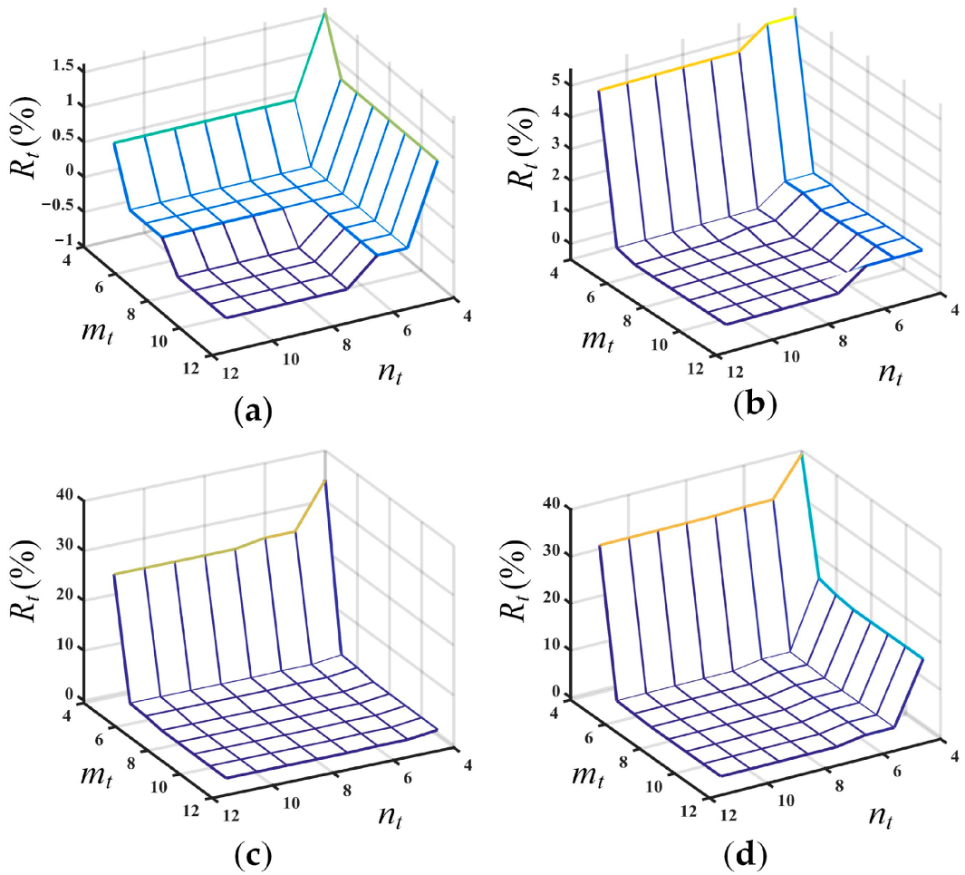
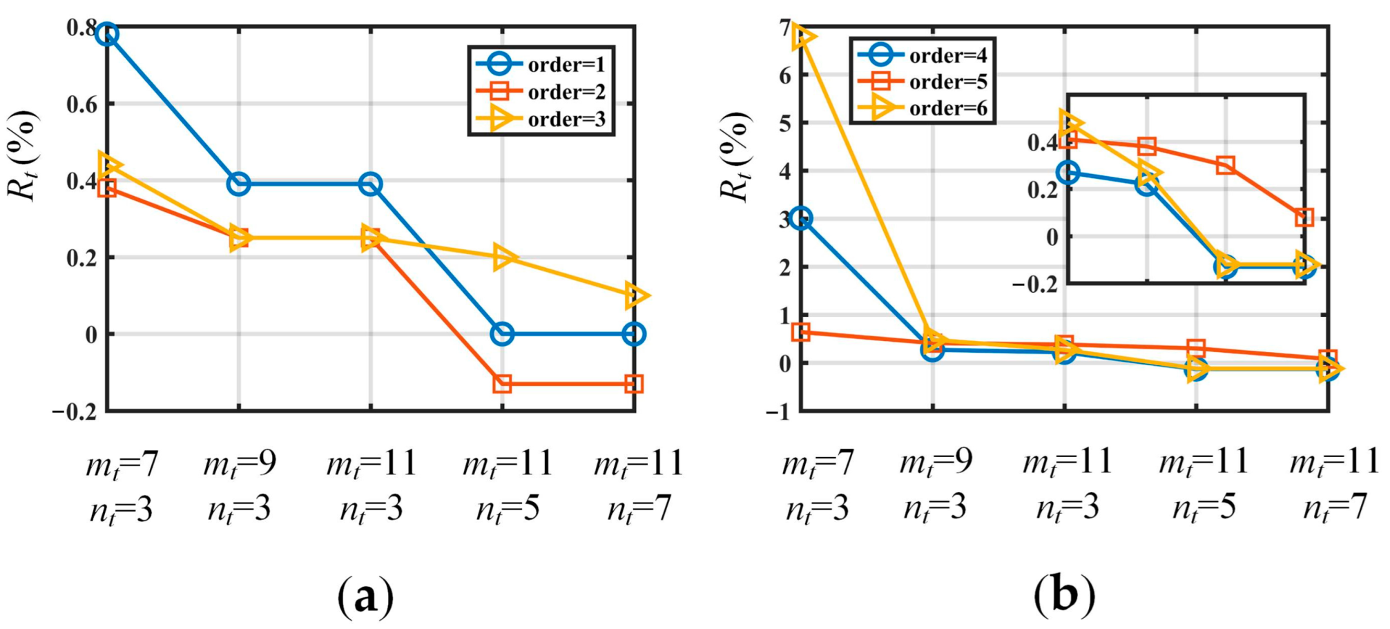
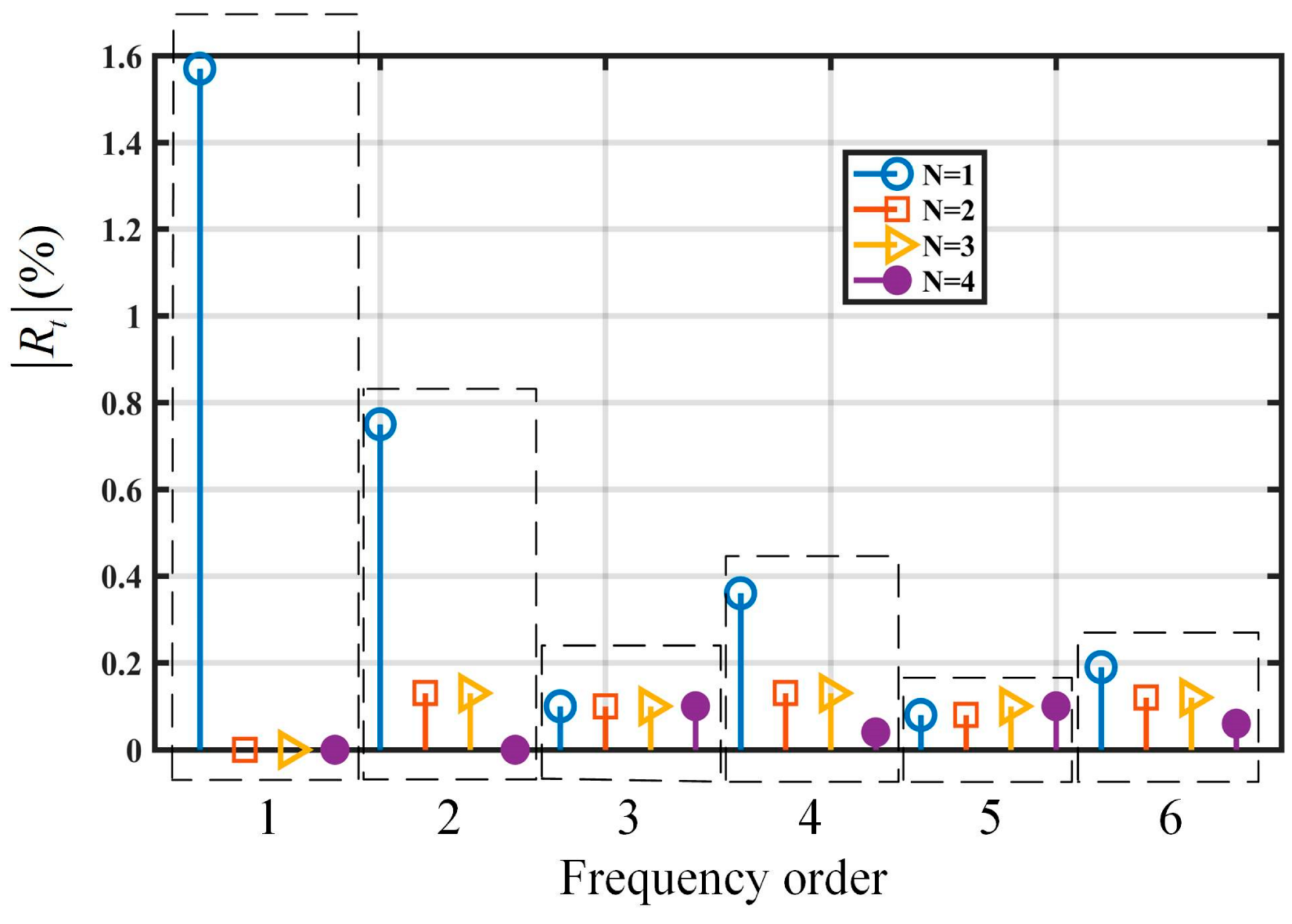
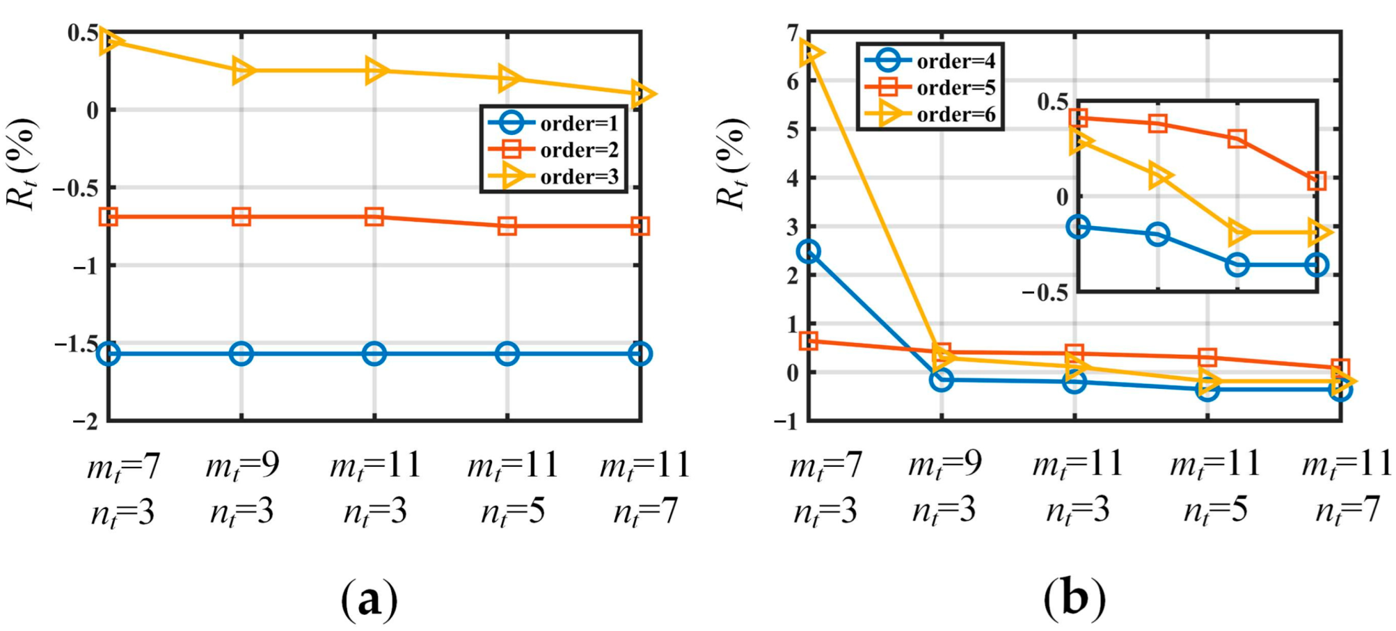
4.2. Study of the Order of Power Series Multipliers

It can be seen from Figure 8 that with the increase of m_t and n_t, the relative errors R_t of the first six frequencies all show a downward trend. The relative errors R_t of the 1st, 2nd, 3rd, and 5th order frequencies are all within 2%. In this m_t = 7 and n_t = 3, the relative error R_t of the 4th and 6th order frequencies is greater than 2%. However, with the increase of m_t and n_t, the relative error R_t will quickly decrease to less than 1%. It can be seen from Figure 9 that with the increase of m_t and n_t, the relative errors R_t of the first six frequencies all show a downward trend. The relative errors R_t of the 1st, 2nd, 3rd, and 5th order frequencies are all within 1%. In this m_t = 7 and n_t = 3, the relative error R_t of the 4th and 6th order frequencies is greater than 2%. However, with the increase of m_t and n_t, the relative error R_t will quickly decrease to less than 1%.

Figure 8 and Figure 9 both show that with the increase of m_t and n_t, the calculated results of the method in this paper converge well. Comparing Figure 8 with Figure 9, it can also be found that the convergence effect is better when the power series multipliers order N = 2 than that of N = 1.

As shown in

Table 5. Influence of the change of truncation coefficient m_t and n_t on the relative frequency error (L = 8 m, 2b = 2 m, N = 3).

Order	ANSYS	Method					Relative Tolerance (%)
		mt = 7 nt = 3	mt = 9 nt = 3	mt = 11 nt = 3	mt = 11 nt = 5	mt = 11 nt = 7
1	0.255	-	-	-	0.255	0.255	-	-	-	0.00	0.00
2	1.595	-	-	-	1.593	1.593	-	-	-	−0.13	−0.13
3	2.031	-	-	-	2.035	2.033	-	-	-	0.20	0.10
4	4.482	-	-	-	4.476	4.476	-	-	-	−0.13	−0.13
5	6.278	-	-	-	6.297	6.284	-	-	-	0.30	0.10
6	8.825	-	-	-	8.814	8.814	-	-	-	−0.12	−0.12
7	11.051	-	-	-	11.102	11.059	-	-	-	0.46	0.07
8	14.647	-	-	-	14.720	14.719	-	-	-	0.50	0.49

, this method fails in this N = 3 and the truncation coefficient n_t = 3. However, with the increase of n_t, this method continues to be effective. The relative error R_t of frequencies is within 1%. Therefore, it can be known that n_t has to be at least greater than 3 when N > 2.

It can be seen from Figure 10 that in the multiplier order of the power series N = 1, the relative error R_t of the 1st, 2nd, and 4th order frequencies is large. This indicates poor convergence when multiplier order N = 1. In this multiplier order N = 2, N = 3, and N = 4, and the relative error R_t of each order frequency is basically the same, all within 0.2%. That means that the convergence is good when the power series multipliers are N = 2, N = 3, and N = 4. It is widely known that the expression with fewer terms has minimal calculation. Hence, it makes sense to choose N = 2 for the power series multiplier order.

4.3. Study on the Frequency of Flexible Spacecraft by This Method

The geometric and material parameters of the spacecraft with a pair of solar panels studied in this paper are shown in

Table 6. Geometrical parameters and material parameters of spacecraft.

Component	Parameter	Values
Solar energy panel	Length L (m)	4, 8, 20, 32
	Width 2b (m)	2
	Thickness 2h (m)	0.02
	Elastic modulus of aluminum E (Pa)	6.89 × 1010
	Mass density of aluminum ρ (kg∙m−3)	2.8 × 103
	Poisson ratio μ	0.33
Center of the rigid body	Half of the side length r0 (m)	1
	The moment of inertia Jx, Jy, Jz (kg∙m2)	100, 100, 100
	The mass of the rigid body mR	150

. Some parameters of solar panels refer to Ref. [14].

As shown in

Table 7. Frequency comparison of the first eight orders of flexible spacecraft f (Hz) (L = 8 m, 2b = 2 m, N = 2).

Order	mt = 9 nt = 3			mt = 11 nt = 5			mt = 11 nt = 7
	Ref. [14]	Method	Rt (%)	Ref. [14]	Method	Rt (%)	Ref. [14]	Method	Rt (%)
1	0.364	0.364	0.00	0.363	0.362	−0.28	0.363	0.362	−0.28
2	0.913	0.914	0.11	0.912	0.912	0.00	0.912	0.911	−0.11
3	2.164	2.165	0.05	2.160	2.156	−0.19	2.160	2.156	−0.19
4	2.659	2.660	0.04	2.652	2.647	−0.19	2.652	2.646	−0.23
5	2.683	2.683	0.00	2.683	2.683	0.00	2.681	2.680	−0.04
6	2.830	2.831	0.04	2.830	2.830	0.00	2.829	2.827	−0.07
7	5.978	5.981	0.05	5.966	5.957	−0.15	5.966	5.957	−0.15
8	6.272	6.277	0.08	6.258	6.246	−0.19	6.257	6.246	−0.18

, the comparison between the first eighth order frequencies of the flexible spacecraft calculated by the presented method and the result of reference [14] is given. By comparison, it can be seen that the relative error R_t of frequency is very small under different truncation coefficients m_t and n_t, which are all kept within 0.3%. The results show the excellent convergence of the presented method. Therefore, it is feasible to install a pair of four-sided free solar panels on the central rigid body by the power series multiplier method. The results show that the flexible spacecraft modeled by this method can replace the flexible spacecraft with a pair of cantilever solar panels installed directly.

As shown in

Table 8. First eight order frequencies of flexible spacecraft with solar panels of different lengths f (Hz) (m_t = 11, n_t = 7, 2b = 2 m, N = 2).

	Order	1	2	3	4	5	6	7	8
L = 4	Ref. [14]	1.420	2.244	5.781	5.937	8.592	9.063	18.863	18.934
	Method	1.414	2.236	5.773	5.929	8.573	9.040	18.840	18.911
	Rt (%)	−0.42	−0.36	−0.14	−0.13	−0.22	−0.25	−0.12	−0.12
L = 8	Ref. [14]	0.363	0.912	2.160	2.652	2.681	2.829	5.966	6.257
	Method	0.362	0.911	2.156	2.646	2.680	2.827	5.957	6.246
	Rt (%)	−0.28	−0.11	−0.19	−0.23	−0.04	−0.07	−0.15	−0.18
L = 20	Ref. [14]	0.062	0.205	0.354	0.629	0.957	1.029	1.163	1.244
	Method	0.062	0.205	0.354	0.629	0.956	1.029	1.163	1.243
	Rt (%)	0.00	0.00	0.00	0.00	−0.10	0.00	0.00	−0.08
L = 32	Ref. [14]	0.025	0.085	0.142	0.270	0.377	0.551	0.637	0.728
	Method	0.025	0.085	0.142	0.270	0.377	0.551	0.637	0.727
	Rt (%)	0.00	0.00	0.00	0.00	0.00	0.00	0.00	−0.14

, the first eight order frequencies of flexible spacecraft with solar panels of different lengths are studied. As can be seen from the table, the relative frequency error R_t is very small for different lengths L of solar panels, which are all kept within 0.5%. With the increase of the solar panel length L, the relative errors of the first eight frequencies R_t tend to decrease. In the solar panel length L = 32 m, the relative error R_t of the first seven order frequency is nearly zero. In fact, the solar panel is presented as a beam when the length is 32 m. This indicates that the frequency of the flexible spacecraft calculated by this method is very close to that of reference [14]. That means when the $L>2b$ of the solar panel is obtained, the result of the power series multiplier method has a very good convergence.

5. Conclusions

In this paper, the power series multiplier constraining method is proposed. It can help to establish a cantilever plate under the boundary condition of the four-sided free plate. Next, the rigid-flexible coupling dynamical model of a flexible spacecraft equipped with a pair of solar panels symmetrically (namely, a central rigid body-flexible plate system) was established. The effectiveness and convergence of the method are verified by comparing the calculation results of the constructed cantilever plate with those of the finite element software ANSYS. Through the analysis of the dynamic characteristic, the main conclusions are summarized as follows:

(1).

Through the study of the natural characteristics of the cantilever plate, it can be known that the convergence of the method is good and the computational efficiency is high in this the power series multiplier order N = 2. Under this condition, when the length of the clamped edge is shorter than that of the adjacent edge, the result is reasonable and accurate. On the contrary, if the length of the clamped edge is obviously longer than that of the adjacent edge, the result is imprecise.

(2).

The method can be extended to a flexible spacecraft equipped with a pair of solar panels symmetrically. By comparing the result with the reference, it can be known that the presented method is not only fit for the single plate, but also feasible for the rigid-flexible coupling structure. It should be mentioned that when the solar panel is so long that it presents as a beam, the convergence of this method is much better. The proposed method can be adopted to the structure, with edges subjected to discontinuous constraints.

References

1. Liu, L.; Cao, D.Q.; Wei, J.; Tan, X.J.; Yu, T.H. Rigid-Flexible Coupling Dynamic Modeling and Vibration Control for a Three-Axis Stabilized Spacecraft. J. Vib. Acoust. 2017, 139, 041006. [Google Scholar] [CrossRef]
2. Li, Q.; Ma, X.R.; Wang, T.S. Reduced Model for Flexible Solar Sail Dynamics. J. Spacecr. Rocket. 2011, 48, 446–453. [Google Scholar] [CrossRef]
3. Liu, L.; Sun, S.P.; Cao, D.Q.; Liu, X.Y. Thermal-structural analysis for flexible spacecraft with single or double solar panels: A comparison study. Acta Astronaut. 2019, 154, 33–43. [Google Scholar] [CrossRef]
4. Li, Y.Y.; Yang, Y.; Li, M.; Liu, Y.F.; Huang, Y.F. Dynamics analysis and wear prediction of rigid-flexible coupling deployable solar array system with clearance joints considering solid lubrication. Mech. Syst. Signal Processing 2022, 162, 108059. [Google Scholar] [CrossRef]
5. Li, Y.Y.; Wang, Z.L.; Wang, C.; Huang, W.H. Planar rigid-flexible coupling spacecraft modeling and control considering solar array deployment and joint clearance. Acta Astronaut. 2018, 142, 138–151. [Google Scholar] [CrossRef]
6. Li, Y.Y.; Li, M.; Liu, Y.F.; Geng, X.Y.; Cui, C.B. Parameter optimization for torsion spring of deployable solar array system with multiple clearance joints considering rigid–flexible coupling dynamics. Chin. J. Aeronaut. 2022, 35, 509–524. [Google Scholar] [CrossRef]
7. Pan, K.Q.; Liu, J.Y. Investigation on the choice of boundary conditions and shape functions for flexible multi-body system. Acta Mech. Sin. 2011, 28, 180–189. [Google Scholar] [CrossRef]
8. Zhang, J.L.; Lu, S.B.; Zhao, L.Y. Modeling and disturbance suppression for spacecraft solar array systems subject to drive fluctuation. Aerosp. Sci. Technol. 2021, 108, 106398. [Google Scholar] [CrossRef]
9. Yang, J.Y.; Liu, F. Coupled Structure Vibration–Attitude Dynamics Evolution and Control of China’s Space Station. Int. J. Aeronaut. Space Sci. 2019, 20, 126–138. [Google Scholar] [CrossRef]
10. Nicassio, F.; Fattizzo, D.; Giannuzzi, M.; Scarselli, G.; Avanzini, G. Attitude dynamics and control of a large flexible space structure by means of a minimum complexity model. Acta Astronaut. 2022, 198, 124–134. [Google Scholar] [CrossRef]
11. Wei, J.; Cao, D.Q.; Liu, L.; Huang, W.H. Global mode method for dynamic modeling of a flexible-link flexible-joint manipulator with tip mass. Appl. Math. Model. 2017, 48, 787–805. [Google Scholar] [CrossRef]
12. Wei, J.; Cao, D.Q.; Huang, H.; Wang, L.C.; Huang, W.H. Dynamics of a multi-beam structure connected with nonlinear joints: Modelling and simulation. Arch. Appl. Mech. 2018, 88, 1059–1074. [Google Scholar] [CrossRef]
13. Fang, B.; Cao, D.Q.; Chen, C.; Chen, S. Nonlinear dynamic modeling and responses of a cable dragged flexible spacecraft. J. Frankl. Inst. 2022, 359, 3238–3290. [Google Scholar] [CrossRef]
14. Liu, L.; Cao, D.Q.; Tan, X.J. Studies on global analytical mode for a three-axis attitude stabilized spacecraft by using the Rayleigh–Ritz method. Arch. Appl. Mech. 2016, 86, 1927–1946. [Google Scholar] [CrossRef]
15. Liu, L.; Cao, D.Q.; Wei, J. Rigid-flexible coupling dynamic modeling and vibration control for flexible spacecraft based on its global analytical modes. Sci. China Technol. Sci. 2018, 62, 608–618. [Google Scholar] [CrossRef]
16. Chen, L.H.; Cui, S.J.; Jing, H.; Zhang, W. Analysis and modeling of a flexible rectangular cantilever plate. Appl. Math. Model. 2020, 78, 117–133. [Google Scholar] [CrossRef]
17. Cao, Y.T.; Cao, D.Q.; Huang, W.H. Dynamic modeling and vibration control for a T-shaped bending and torsion structure. Int. J. Mech. Sci. 2019, 157–158, 773–786. [Google Scholar] [CrossRef]
18. Cao, Y.T.; Cao, D.Q.; Liu, L.; Huang, W.H. Dynamical modeling and attitude analysis for the spacecraft with lateral solar arrays. Appl. Math. Model. 2018, 64, 489–509. [Google Scholar] [CrossRef]
19. Cao, Y.T.; Cao, D.Q.; He, G.Q.; Liu, L. Thermal alternation induced vibration analysis of spacecraft with lateral solar arrays in orbit. Appl. Math. Model. 2020, 86, 166–184. [Google Scholar] [CrossRef]
20. He, G.Q.; Cao, D.Q.; Cao, Y.T.; Huang, W.H. Investigation on global analytic modes for a three-axis attitude stabilized spacecraft with jointed panels. Aerosp. Sci. Technol. 2020, 106, 106087. [Google Scholar] [CrossRef]
21. Xing, W.C.; Wang, Y.Q. Vibration characteristics analysis of rigid-flexible spacecraft with double-direction hinged solar arrays. Acta Astronaut. 2022, 193, 454–468. [Google Scholar] [CrossRef]
22. He, G.Q.; Cao, D.Q.; Wei, J.; Cao, Y.T.; Chen, Z.G. Study on analytical global modes for a multi-panel structure connected with flexible hinges. Appl. Math. Model. 2021, 91, 1081–1099. [Google Scholar] [CrossRef]
23. He, G.Q.; Cao, D.Q.; Cao, Y.T.; Huang, W.H. Dynamic modeling and orbit maneuvering response analysis for a three-axis attitude stabilized large scale flexible spacecraft installed with hinged solar arrays. Mech. Syst. Signal Processing 2022, 162, 108083. [Google Scholar] [CrossRef]
24. Cao, Y.T.; Cao, D.Q.; He, G.Q.; Ge, X.S.; Hao, Y.X. Modelling and vibration analysis for the multi-plate structure connected by nonlinear hinges. J. Sound Vib. 2021, 492, 115809. [Google Scholar] [CrossRef]
25. Xing, W.C.; Wang, Y.Q. Vibration characteristics of thin plate system joined by hinges in double directions. Thin-Walled Struct. 2022, 175, 109260. [Google Scholar] [CrossRef]
26. Bhat, R.B. Natural frequencies of rectangular plates using characteristic orthogonal polynomials in Rayleigh–Ritz method. J. Sound Vib. 1985, 102, 493–499. [Google Scholar] [CrossRef]
Figure 1. Schematic diagram of the cantilever plate.
Actuators 12 00003 g001
Figure 2. Constraint types described by different methods (left is the traditional Lagrange method, right is the method in this paper. Left view).
Actuators 12 00003 g002
Figure 3. Flexible spacecraft model.
Actuators 12 00003 g003
Figure 4. Variation of relative frequency error with the number of intercepted orthogonal polynomials (L = 8 m, 2b = 8 m, N = 2): (a) the 1st order frequency; (b) the 2nd order frequency; (c) the 3rd order frequency; (d) the 4th order frequency.
Actuators 12 00003 g004
Figure 5. Comparison of the first six order frequency relative errors Rt (M and A represent the relative errors between the calculated results of the proposed method and those of the finite element software ANSYS, M and T represent the relative errors between the calculated results of the proposed method and those of the traditional characteristic orthogonal polynomial method. mt = 11, nt = 7, N = 2): (a) L = 8 m, 2b = 2 m; (b) L = 2 m, 2b = 4 m.
Actuators 12 00003 g005
Figure 6. The first eight modes of the plate (left is the result of the traditional method, middle is the result of the method in this paper, right is the result of ANSYS. L = 8 m, 2b = 2 m, mt = 11, nt = 7, N = 2): (a) the 1st mode; (b) the 2nd mode; (c) the 3rd mode; (d) the 4th mode; (e) the 5th mode; (f) the 6th mode; (g) the 7th mode; (h) the 8th mode.
Actuators 12 00003 g006
Figure 7. The 4th, 6th, 7th, and 8th modes of the plate (left is the result of the traditional method, middle is the result of the method in this paper, right is the result of ANSYS. L = 2 m, 2b = 4 m, mt = 11, nt = 7, N = 2): (a) the 4th mode; (b) the 6th mode; (c) the 7th mode; (d) the 8th mode.
Actuators 12 00003 g007
Figure 8. Influence of the change of truncation coefficient mt and nt on the relative frequency error (L = 8 m, 2b = 2 m, N = 1): (a) the 1st, 2nd, and 3rd order frequencies; (b) the 4th, 5th, and 6th order frequencies.
Actuators 12 00003 g008
Figure 9. Influence of the change of truncation coefficient mt and nt on the relative frequency error (L = 8 m, 2b = 2 m, N = 2): (a) the 1st, 2nd, and 3rd order frequencies; (b) the 4th, 5th, and 6th order frequencies.
Actuators 12 00003 g009
Figure 10. Influence of power series multiplier order N on frequency relative error (L = 8 m, 2b = 2 m, mt = 11, nt = 7).
Actuators 12 00003 g010