Dynamics and Computed-Muscle-Force Control of a Planar Muscle-Driven Snake Robot

Abstract

This paper presents the dynamic formulation of an artificial-muscle-driven and computed-muscle–force control for the planar locomotion of a snake robot. The snake robot uses a series of antagonistic pneumatic artificial muscles, assembled at the joints, to generate the locomotion. Kinematics of the artificial-muscle-driven robot in the joint and Cartesian spaces was derived with respect to the muscles’ motion. The Lagrangian mechanics was employed for the formulation of the dynamic model of the robot and deriving the equations of motion. A model-based computed-muscle-force control was designed to track the desired paths/trajectories in Cartesian space. The feedback linearization method based on a change of coordinate was utilized to determine an equivalent linear (input-to-state) system. Then, a full state feedback control law was designed, which satisfies the stability and tracking problems. The performance of the dynamic model and the controller were successfully demonstrated in simulation studies for tracking a circle-shape path and a square-shape path with a constant linear velocity while generating the lateral undulation gait. The results indicate a low magnitude of tracking errors where the controlled muscle force are bounded to the actual pneumatic artificial muscle’s limitations.

1. Introduction

Since the pioneering work by Professor Shigeo Hirose [1], who developed the first snake-like robot at Tokyo Institute of Technology, biological snakes and similar limbless animals have fascinated roboticists over half a century due to their vast abundance in a variety of environments (land, sea, and even gliding in the air [2]) as well as their versatile locomotion that adapts easily to unstructured and unknown environments [3,4]. Snake-like robots, in contrast to their biological counterparts, have shown limitations for agile mobility, long range navigation, and surveying the field with a large area mainly due to the low energy-consumption-efficiency and low power-to-weight ratio [2]. Most snake robots that have been designed and developed thus far use motorized joints for generating locomotion. The recent advancements in soft robotics help to enhance the capabilities of robotic systems by designing and developing snake robots [5,6,7,8,9,10] with compliant and structurally deformable bodies that generate more complex motion while reducing the cost, weight, and complexity of the mechanical structures [11]. That leads to potential solutions for addressing energy consumption while creating more complex motion.

An extensive body of research has been conducted on studying the dynamics, control, motion planning, and design of snake robots [1,12,13,14,15,16]. Chirikjian and Burdick introduced an integral form of continuous backbone curves for solving the inverse kinematics of hyper-redundant robot locomotion with nonholonomic constraints following desired trajectories [12]. Wright et al. designed a modular snake robot capable of climbing inside and outside of pipes [13]. Ma [14] studied the creeping locomotion of the snake robot using the Serpentine curve in a constant steady-state velocity. A mathematical framework was established in [15] for the modeling, analysis, and synthesis of serpentine locomotion with a multi-link robotic snake without wheels that facilitates adapting to the environment at the expense of power efficiency. Tanaka and Matsuno proposed a control of snake robot that lift its parts of its body and dynamically switch lifting parts during locomotion which facilitates rapid and efficient movement across a sandy surface [16]. For a comprehensive review and list of research efforts on snake robots, the reader is referred to review papers and books [2,17]. Different dynamic modeling approaches have been utilized for modeling snake robots. Creep locomotion of snake robot on inclined surfaces without non-holonomic constrains was modeled [14]. Kane’s dynamic formulation method [18,19,20] and the articulated body algorithm [21,22,23] were employed for computationally efficient modeling. Guo and Mahadaven [24] developed the governing equations for the planar lateral undulation of a continuum model of a snake robot, modeled as a thin filament, integrated with internal muscles that interacts with its surrounding environment. A geometric formulation was developed for studying a kinematic connection that decouples the low-dimensional net locomotion from the high-dimensional serpentine locomotion [25]. Modeling the transversal link displacement was introduced to derive a simpler model for a snake robot locomotion instead of the commonly used joint motion-based modeling approach [2,17].

From a control point of view, many research efforts were dedicated to the pattern gait control of snake robots [2,12,17,26,27,28,29] with some work studied on the position/heading direction while considering side-slip constraints (nonholonomic) [30]. Ma used the Serpenoid curve equations and the body shape change with respect to the time variation of the Serpenoid curve for controlling the heading direction and the locomotion speed of the snake robot [26]. Xiao et al., in [27], proposed a locomotive reduction approach based on the average body framework, which reduces the complexity of controlling a redundant snake robot to that of navigating a differential-drive vehicle. Hatton and Choset [28] introduced two gate generator approaches, called Annealed chain fitting and Keyframe wave extraction, that maps between the 3D shape of a snake robot’s backbone curve and a set of joint angles and vice versa to address the gate design problems in snake robots. Ostrowski and Burdick [29] used geometric mechanics to describe the net motion of the snake robot as a function of variations in the body shape variables. Hicks and Ito [31] has studied the determination of optimal gaits for the control of position/heading direction for the locomotion of snake robots without side-slip constraints on a flat surface; however, the velocity control was not considered. A kinematic-based controller was studied that exploits the redundancy of a 3D snake robot for controlling its position and posture [32]. Sliding-mode controller were developed to modulate the internal body motion and to generate the required serpentine locomotion by attenuating the lateral slip at each link to follow desired trajectories while compensate for uncertainties regarding the model and the environment parameters such as mass and friction coefficients [18,19]. Moreover, maneuvering control of land-based [33] and underwater [34] snake robots were investigated by enforcing a virtual holonomic constraint to produce the undulatory locomotion. In related works, a combined heading-velocity control based on undulatory gait parameters was studied for autonomous navigation and obstacle avoidance of a planar snake robot [21,22]. Liljeback et al. [17] introduced a combined control with three components, a body wave component (adjust force propulsion), a shape adapt component (adjust the body shape to the environment for obstacle-aided locomotion), and a heading direction control component for steering the snake robot. Chang et al. [35] developed a combined optimal trajectory synthesis strategy and a feedback controller for collision avoidance to adjust the snake robot’s body shape for passing through narrow and confined spaces. A combined shape-velocity-heading strategy based on a variation of the lateral undulation gait parameters was studied for the maneuvering control of snake robot locomotion in navigating confined spaces with varying widths [23].

In recent years, there has been an increasing interest in studying bio-hybrid robots, which integrate living cells (e.g., excised or cultured muscle) coupled to a robot’s structure to generate enhanced motion and force [36,37]. This promising concept relies on this fact that biological muscles, seamlessly integrated with sensorimotor controls, are ideal actuators with superior performance metrics. On the other hand, Pneumatic Artificial Muscles (PAMs), also known as the McKibben muscle [38], have shown to be promising in improving energy consumption efficiency compared to other actuators while generating a high power-to-weight ratio, a force-to-volume ratio, and a moderate to high order of force [38,39,40,41,42]. Similarities between the biomechanics of artificial muscles and natural muscles have made these actuators a feasible option for a variety of robotics applications including biomimemtic robots [39,43], human–robot interaction [44], assistive and rehabilitation robotic exoskeletons [41,45,46,47,48], and robotic manipulators [42]. However, most of these applications are limited to immobile platforms [39,49]. The anatomy of natural snakes and particularly their musculoskeletal structure, which is composed of 130 to 435 vertebrae along with attached antagonist axial muscle configurations [14,50,51], can be considered as a series of rigid links hinged together, whilst axial musculature can be regarded as a series of elastic elements operating laterally to the hinges and between adjacent links. During lateral undulation locomotion, snakes alternately activate these antagonistic muscles on either side of their body to active flexural movement [24,52,53,54]. The use of similar antagonistic mechanisms has been explored and studied for snake robots such as a tendon-driven antagonist mechanism for snake locomotion [51] and a snake-like surgical robot [55]. An “integrated joint actuator”, a set of pneumatic bellows attached to links between a serpentine robot (OmniTread OT-4), which generate a 2 DOF motion, was introduced by Granosik and Borenstien [56]. Parallel elastic actuators (PEA), which combine an actuator (e.g., an electrical motor at the joint) and spring element in a parallel configuration, has been exploited for energy-efficient locomotion of snake robots [57,58].

In our previous work [59], an artificial-muscle-driven snake robot was introduced, which uses a series of antagonistic PAMs, assembled lateral to the joints, where alternate activation of the antagonistic muscles generate the internal body motion and consequently the external locomotion due interaction with its surrounding environment. Based on experimental and analytical studies and their characterizations, it was demonstrated that the kinematic and dynamic performances of the snake robots are comparable to the current state-of-the-art snake-like robots, and, in some aspects, even exceed them.

This work presents the mathematical formulation for the kinematics and dynamics of a planar artificial-muscle-driven snake robot with respect to the muscles’ motion and force. The Lagrangian mechanics was employed to derive the equations of motion with muscle forces as inputs to the dynamical system. A model-based computed muscle–force–controller was designed to facilitate the tracking of the desired paths with different geometrical and topological features in Cartesian space while generating the lateral undulation gate in the body joint space. Feedback linearization was utilized based on a change of coordinate to derive an equivalent linear input-to-state system. Next, a full state-feedback control law was designed, which satisfies the asymptotic stability of the snake robot in tracking desired trajectories. Simulation studies were carried in MATLAB on a model of a six-link snake robot.

The organization of this paper is as follows. Section 2 presents the kinematics of the snake robot in terms of the muscle’s motion, and overall mapping between the joint space and Cartesian space configurations will be discussed. Moreover, the dynamics of a N-Link snake robot based on the Lagrangian mechanics is derived. Additionally, the design of a computed-muscle–force controller is discussed where the model-based feedback linearization and full state feedback control laws are formulated. Finally, Section 3 presents and discusses the results obtained for two simulation case studies using a six-link snake robot model for tracking a circle-shape path and a square-shape path.

2. Materials and Methods

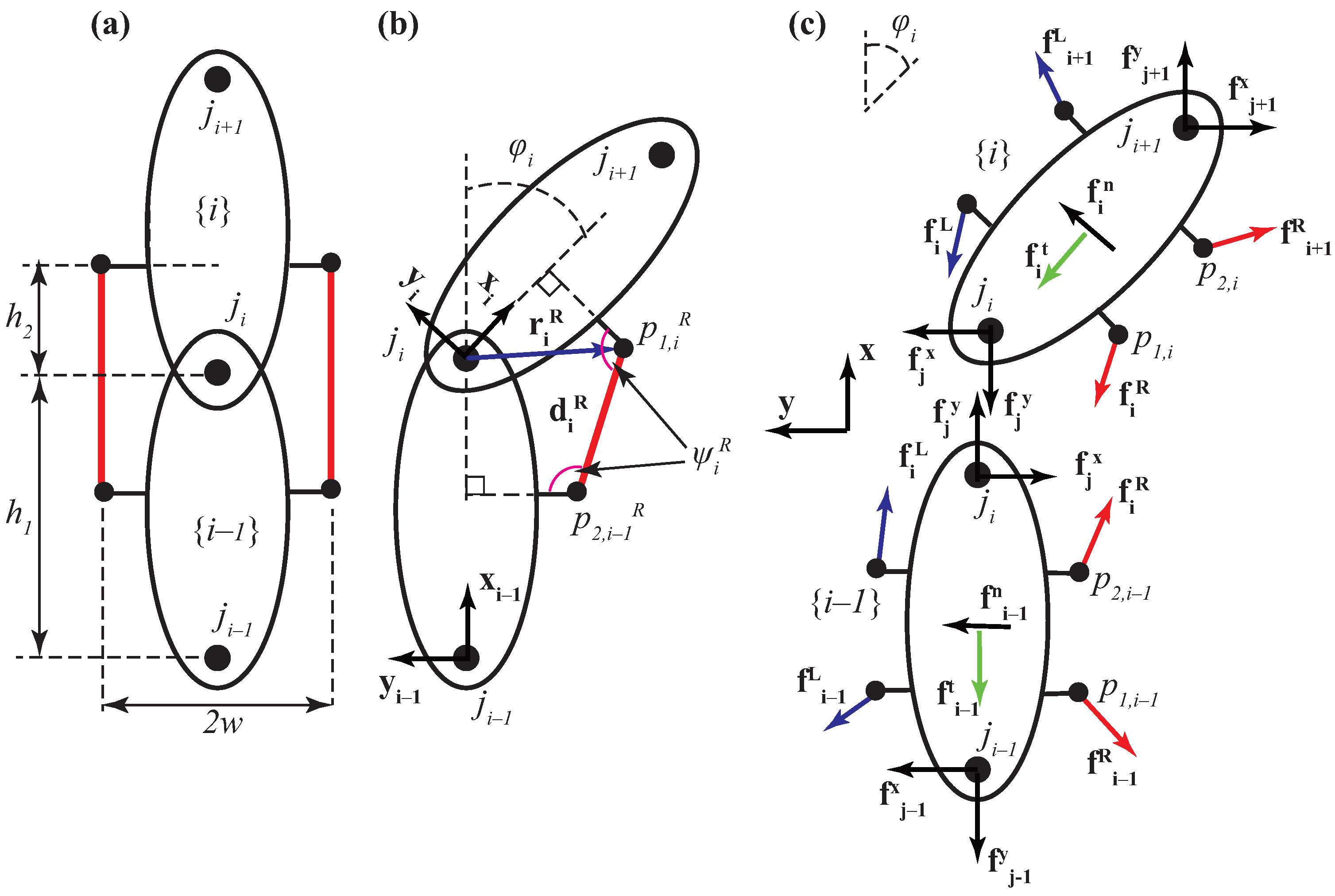
2.1. Kinematics of Artificial-Muscle-Driven Snake Robot

The kinematics of robots is generally described through the mapping between three configuration spaces, actuator, joint, and Cartesian/operational spaces. Herein, the interrelationship between these three spaces for the snake robot was discussed to develop kinematic models, which will be used for the dynamic modeling and control of snake robots in the future.

2.1.1. Joint Position–Muscle Vector Relationship

The relationship between the muscle movement and joint position of a snake robot was developed and studied. As illustrated in Figure 1a, the muscles are attached to the links of the snake robot at two points on the right-side and two points on the left-side, where the muscle can freely rotate about those two points which keeps it straight during the rotation of the joint. To describe the motion of each muscle, the position vectors of the connecting points, $p_{2,i-1}^R$ and $p_{1,i}^R$, on the right side, are defined with respect to the body frame $\left\{i\right\}$ at the joint $\{i-1\}$, and are obtained as follows

$$\begin{array}{ccc}\hfill {}^{i-1}{\mathbf{r}}_{p_{1,i}}& =& \hfill \left[\begin{array}{c}{h}_1+h_{2}cos\left({\varphi }_i\right)+wsin\left({\varphi }_i\right)\\ h_{2}sin\left({\varphi }_i\right)-wcos\left({\varphi }_i\right)\end{array}\right]\hfill \end{array}$$

(1)

$$\begin{array}{ccc}\hfill {}^{i-1}{\mathbf{r}}_{p_{2,i-1}}& =& \hfill \left[\begin{array}{c}{h}_1-h_2\\ -w\end{array}\right]\hfill \end{array}$$

(2)

where $h_1$, $h_2$, w, and ${\varphi }_i$ are the length of each link, distance from the joint to the attachment point, half width of each link, and the joint angle, as shown in Figure 1a,b, respectively.

The vector ${\mathbf{d}}_i$ connecting these two points, corresponding to the muscle and called a muscle vector, can be obtained as

$${\mathbf{d}}_i={}^{i-1}{\mathbf{r}}_{p_{1,i}}-{}^{i-1}{\mathbf{r}}_{p_{2,i-1}}=\left[\begin{array}{c}{h}_2(1+cos\left({\varphi }_i\right))+wsin\left({\varphi }_i\right)\\ h_{2}sin\left({\varphi }_i\right)+w(1-cos\left({\varphi }_i\right))\end{array}\right]$$

(3)

Equation (3) can be written in the following form,

$${\mathbf{d}}_i=(I+\overline{R}\left({\varphi }_i\right))\mathbf{g}=\mathcal{D}\left({\varphi }_i\right)\mathbf{g}$$

(4)

where $I\in {\mathbb{R}}^{2\times 2}$ is an identity matrix, $\overline{R}\left({\varphi }_i\right)\in O\left(2\right)$ is an improper rotation matrix, i.e., $det\left(\overline{R}\right)=-1$ in terms of the joint angle, and $\mathbf{g}$ is a constant vector, which includes geometric information of the link given by

$$\overline{R}\left({\varphi }_i\right)=\left[\begin{array}{cc}cos\left({\varphi }_i\right)& sin\left({\varphi }_i\right)\\ sin\left({\varphi }_i\right)& -cos\left({\varphi }_i\right)\end{array}\right]$$

$$\mathbf{g}=\left[\begin{array}{c}{h}_2\\ w\end{array}\right]$$

we define $\mathcal{D}:{\mathbb{R}}^2\to {\mathbb{R}}^2$ as an operator that maps a geometric vector $\mathbf{g}$ to a muscle vector $\mathbf{d}$. Note that $\overline{R}\left({\varphi }_i\right)$ is symmetric (i.e., ${\overline{R}}^T=\overline{R}$) in addition to all other properties of special orthogonal matrices $O\left(2\right)$. Therefore, the operator $\mathcal{D}$ has the following multiplicative properties

$$\begin{array}{cc}\hfill {\mathcal{D}}^T\mathcal{D}& \hfill =2\mathcal{D}\hfill \end{array}$$

(5)

$$\begin{array}{cc}\hfill {\mathcal{D}}^n& \hfill =2^{n-1}\mathcal{D}\hfill \end{array}$$

(6)

which will be used through all kinematics’ and dynamics’ derivation. The length of the muscle vector ${\mathbf{d}}_i$ can be obtained by

$${\ell }_i^2=2{\mathbf{g}}^T\mathcal{D}\left({\varphi }_i\right)\mathbf{g}$$

(7)

where the relationship between the joint angle and the length of the PAMs is given by

$${\ell }_i^2=(2h_2^2-2w^2)cos\left({\varphi }_i\right)+4h_{2}wsin\left({\varphi }_i\right)+2h_2^2+2w^2$$

(8)

Solving Equation (8) for the joint position, ${\varphi }_i$, yields

$${\varphi }_i={\Phi }_i\left({\ell }_i^2\right)={tan}^{-1}(\frac{h_2^2-w^2}{2h_{2}w})\pm {tan}^{-1}(\frac{2h_2^2+2w^2-{\ell }_i^2}{\sqrt{{(2h_2^2-2w^2)}^2+{\left(4h_{2}w\right)}^2-{(2h_2^2+2w^2-{\ell }_i^2)}^2}})$$

(9)

Although Equation (9) provides two solutions, based on the feasible range of mechanism motions and a given muscle length, a unique solution will be chosen. The linear velocity and acceleration of the muscle vector ${\mathbf{d}}_i$ can be obtained by

$${\dot{\mathbf{d}}}_i=\dot{\mathcal{D}}\left({\varphi }_i\right)\mathbf{g}=\left({\mathcal{D}}_i-I\right)S\mathbf{g}{\dot{\varphi }}_i$$

(10)

$${\ddot{\mathbf{d}}}_i=S\mathbf{g}{\ddot{\varphi }}_i-I\mathbf{g}{\dot{\varphi }}_i^2$$

(11)

where $S\in {\mathbb{R}}^{2\times 2}$ is a skew-symmetric matrix of the following form,

$$S=\left[\begin{array}{cc}0& 1\\ -1& 0\end{array}\right],$$

(12)

and $\dot{\varphi }$ and $\ddot{\varphi }$ are the joint velocity and acceleration, respectively.

From Equation (10), it can be shown that

$${\dot{\varphi }}_i=\frac{1}{{\lambda }_g}{\mathbf{g}}^T{S}^T\left({\mathcal{D}}_i-I\right){\dot{\mathbf{d}}}_i$$

(13)

where ${\lambda }_g={\mathbf{g}}^T\mathbf{g}>0$. By defining the bundle $\tilde{\mathbf{d}}\in {\mathbb{R}}^{2(N-1)}$ and its time-derivative $\dot{\tilde{\mathbf{d}}}$,

$$\tilde{\mathbf{d}}=\left[\begin{array}{c}{\mathbf{d}}_1\\ ⋮\\ {\mathbf{d}}_{N-1}\end{array}\right]$$

(14)

the vector of joint angle velocities $\dot{\varphi }\in {\mathbb{R}}^{N-1}$ can be obtained by,

$$\dot{\varphi }=\mathcal{J}\dot{\tilde{\mathbf{d}}},$$

(15)

where $\mathcal{J}\left(\varphi \right)\in {\mathbb{R}}^{(N-1)\times 2(N-1)}$ given by,

$$\mathcal{J}=\frac{1}{{\lambda }_g}\left[\begin{array}{cccc}{\mathbf{g}}^T{S}^T\left({\mathcal{D}}_1-I\right)& \mathbf{0}& \dots & \mathbf{0}\\ \mathbf{0}& {\mathbf{g}}^T{S}^T\left({\mathcal{D}}_2-I\right)& \dots & \mathbf{0}\\ ⋮& ⋮& ⋮& ⋮\\ \mathbf{0}& \mathbf{0}& \dots & {\mathbf{g}}^T{S}^T\left({\mathcal{D}}_{N-1}-I\right)\end{array}\right].$$

2.1.2. Joint Space to Cartesian Space

To describe the position and orientation of the snake robot links in terms of the joint space variables ${\mathbf{d}}_i$, the forward kinematics of the planar snake robot, as shown in Figure 2, can be derived by writing the velocities for the consecutive links of an open kinematic chain. Note that the artificial-muscle-driven mechanism is not shown in Figure 2 for the sake of clarity. The first joint is modeled as a floating planar joint (two translational and one rotational DOF) and the rest of the joints are one rotational DOF. The snake robot motion in a 2D space is described by the coordinates of the origin of the frame $\left\{1\right\}$ (x and y) attached to the first link of the snake robot and the absolute angle of the links ${\theta }_i$ with respect to the reference frame $\left\{0\right\}$, as shown in Figure 2.

The position of the head of the snake robot is defined by $\mathbf{p}={[x,y]}^T\in {\mathbb{R}}^2$ and the orientation of the links is selected as $\mathbf{\theta }={[{\theta }_1,{\theta }_2,\dots ,{\theta }_N]}^T\in {\mathbb{R}}^N$, a vector of joint angles is defined by $\mathit{\varphi }={[{\varphi }_1,{\varphi }_2,\dots ,{\varphi }_{N-1}]}^T\in {\mathbb{R}}^{N-1}$. The link angles are related to the joint angles by the following relationship,

$$\theta =\mathbf{1}{\theta }_1+H\mathit{\varphi }$$

(16)

where

$$\mathbf{1}=\left[\begin{array}{c}1\\ 1\\ ⋮\\ 1\end{array}\right]\in {\mathbb{R}}^N$$

and

$$H=\left[\begin{array}{ccccc}0& 0& \dots & 0& 0\\ 1& 0& \dots & 0& 0\\ 1& 1& \dots & 0& 0\\ ⋮& ⋮& \ddots & ⋮& ⋮\\ 1& 1& \cdots & 1& 0\\ 1& 1& \cdots & 1& 1\end{array}\right]\in {\mathbb{R}}^{N\times N-1}$$

The angular and linear velocities of each link are defined as follows,

$$\begin{array}{ccc}\hfill {\omega }_1& =& \hfill {\dot{\theta }}_1\hfill \end{array}$$

(17)

$$\begin{array}{ccc}\hfill {\omega }_i& =& \hfill {\dot{\theta }}_{i-1}+{\dot{\varphi }}_{i-1}i=2,\dots ,N\hfill \end{array}$$

(18)

Using Equations (16)–(18), the vector of joint velocities $\mathbf{\omega }\in {\mathbb{R}}^{N-1}$ can be derived as,

$$\mathbf{\omega }=\mathbf{1}{\dot{\theta }}_1+H\dot{\mathbf{\varphi }}$$

(19)

The linear velocities of the snake robot’s links and muscles are

$$\begin{array}{ccc}\hfill {}^0{\mathbf{\upsilon }}_0^j& =& \hfill \dot{\mathbf{p}}{\omega }_0=0\hfill \end{array}$$

(20)

$$\begin{array}{ccc}\hfill {}^i{\mathbf{\upsilon }}_i^j& =& \hfill {}_{i-1}^{i}R\left({}^{i-1}{\mathbf{\upsilon }}_{i-1}^j+\widehat{\mathbf{g}}{\omega }_{i-1}\right)i=1,\dots ,N\hfill \end{array}$$

(21)

$$\begin{array}{ccc}\hfill {}^i{\mathbf{\upsilon }}_i^m& =& \hfill {}^i{\mathbf{\upsilon }}_i^j+\mathbf{g}{\omega }_{i}i=1,\dots ,N\hfill \end{array}$$

(22)

$$\begin{array}{ccc}\hfill {}^i{\mathbf{\upsilon }}_i^C& =& \hfill {}^i{\mathbf{\upsilon }}_i^j+\frac{1}{2}\widehat{\mathbf{g}}{\omega }_{i}i=1,\dots ,N\hfill \end{array}$$

(23)

where,

$$\widehat{\mathbf{g}}=\left[\begin{array}{c}{h}_1\\ 0\end{array}\right].$$

Substituting Equations (20) and (21) into Equation (23) yields,

$${}^i{\mathbf{\upsilon }}_i^C={}_0^{i}R\dot{\mathbf{p}}+\sum _{j=1}^{i-1}{}_j^{i}R\widehat{\mathbf{g}}{\omega }_j+\frac{1}{2}\widehat{\mathbf{g}}{\omega }_{i}i=1,\dots ,N$$

(24)

presently, by defining a bundle of velocity vectors as ${\tilde{\mathbf{\upsilon }}}_C\in {\mathbb{R}}^{2N\times 1}$,

$${\tilde{\mathbf{\upsilon }}}_C=\left[\begin{array}{c}{}^1{\mathbf{\upsilon }}_1^C\\ ⋮\\ {}^N{\mathbf{\upsilon }}_N^C\end{array}\right]$$

(25)

the collection of the vectors, given in Equation (24), can be written in the following compact form,

$${\tilde{\mathbf{\upsilon }}}_C=\mathcal{A}\dot{\mathbf{p}}+\mathcal{B}\omega$$

(26)

where $\mathcal{A}\in {\mathbb{R}}^{2N\times 2}$ and $\mathcal{B}\in {\mathbb{R}}^{2N\times N}$ are given by,

$$\mathcal{A}=\left[\begin{array}{c}{}_0^{1}R\\ ⋮\\ {}_0^{N}R\end{array}\right]$$

and,

$$\mathcal{B}=\left[\begin{array}{ccccc}\frac{1}{2}\widehat{\mathbf{g}}& \mathbf{0}& \mathbf{0}& \dots & \mathbf{0}\\ {}_1^{2}R\widehat{\mathbf{g}}& \frac{1}{2}\widehat{\mathbf{g}}& \mathbf{0}& \dots & \mathbf{0}\\ {}_1^{3}R\widehat{\mathbf{g}}& {}_2^{3}R\widehat{\mathbf{g}}& \frac{1}{2}\widehat{\mathbf{g}}& \dots & \mathbf{0}\\ ⋮& ⋮& ⋮& ⋮& ⋮\\ {}_1^{N}R\widehat{\mathbf{g}}& {}_2^{N}R\widehat{\mathbf{g}}& {}_3^{N}R\widehat{\mathbf{g}}& \dots & \frac{1}{2}\widehat{\mathbf{g}}\end{array}\right].$$

By comparing Equation (22) to (23, a similar relationship can be derived for ${\tilde{\mathbf{\upsilon }}}_m$, as follows,

$${\tilde{\mathbf{\upsilon }}}_m=\mathcal{A}\dot{\mathbf{p}}+\mathcal{G}\mathbf{\omega }$$

(27)

where $\mathcal{G}$ is given as,

$$\mathcal{G}=\left[\begin{array}{ccccc}\mathbf{g}& \mathbf{0}& \mathbf{0}& \dots & \mathbf{0}\\ {}_1^{2}R\widehat{\mathbf{g}}& \mathbf{g}& \mathbf{0}& \dots & \mathbf{0}\\ {}_1^{3}R\widehat{\mathbf{g}}& {}_2^{3}R\widehat{\mathbf{g}}& \mathbf{g}& \dots & \mathbf{0}\\ ⋮& ⋮& ⋮& ⋮& ⋮\\ {}_1^{N}R\widehat{\mathbf{g}}& {}_2^{N}R\widehat{\mathbf{g}}& {}_3^{N}R\widehat{\mathbf{g}}& \dots & \mathbf{g}\end{array}\right].$$

2.2. Dynamics

The dynamic model of a planar model of the snake robot, as shown in Figure 2, with N links connecting N − 1, revolute joints along with the antagonist artificial-muscle-driven mechanism at each joint, was derived. The dynamic model considers the snake robot without the common side-slip constraints (non-holonomic constraints). We assumed that anisotropic friction applied to each link of the snake robot with a friction larger in the normal direction than in the tangential direction along each link. Therefore, the robot has N + 2 degrees-of-freedom (DOF) and is an under-actuated dynamic system where the internal shape motion is no longer directly related to the overall displacement of the snake robot. The forward dynamics of the snake-robot, shown in Figure 2, were derived using the Lagrangian mechanics.

2.2.1. Lagrangian of the Artificial-Muscle-Driven Snake Robot

The generalized coordinates $\mathbf{q}={[q_1,q_2,\dots ,q_N]}^T\in {\mathbb{R}}^N$ are selected where $q_1$, $q_2$, and $q_3$ are the position (i.e., x and y components) and orientation of the first link (${\theta }_1$), respectively, with respect to the fixed reference frame $\left\{0\right\}$. The rest of the generalized coordinates are defined as the function of the muscle vector as follows,

$$q_{k+3}=2{\mathbf{g}}^T{\mathbf{d}}_{k}k=1,2,\dots ,N-1$$

the time-derivative of $q_{k+3}$ can be related to joint velocities by substituting

$${\dot{q}}_{k+3}=2{\mathbf{g}}^T{\dot{\mathbf{d}}}_k={\lambda }_i{\dot{\varphi }}_i$$

(28)

where

$${\lambda }_i=2{\mathbf{g}}^T\left({\mathcal{D}}_i-I\right)S\mathbf{g}$$

presently, for the vector of $\dot{\tilde{\mathbf{q}}}={[{\dot{q}}_4,{\dot{q}}_5,\dots ,{\dot{q}}_{N+2}]}^T$ we have,

$$\dot{\tilde{\mathbf{q}}}=\mathsf{\Lambda }\dot{\varphi }$$

(29)

where $\mathsf{\Lambda }=\mathrm{diag}\{{\lambda }_1,{\lambda }_1,\dots ,{\lambda }_{N-1}\}$ is a diagonal square matrix of ${\mathbb{R}}^{N-1\times N-1}$ with non-zero entries on the main diagonal, thus it is invertible and ${\mathsf{\Lambda }}^{-1}$ exists.

The Lagrangian of the dynamical system can be written as follows [60],

$$\mathcal{L}(\mathbf{q},\dot{\mathbf{q}})=\frac{1}{2}{\tilde{\mathbf{\upsilon }}}_C^T\tilde{M}{\tilde{\mathbf{\upsilon }}}_C+\frac{1}{2}{\mathrm{\omega }}^T{I}_C\mathbf{\omega }$$

(30)

where $\tilde{M}\in {\mathbb{R}}^{N\times N}$ and ${\tilde{I}}_C\in {\mathbb{R}}^{N\times N}$ are given by,

$$\tilde{M}=\left[\begin{array}{ccccc}m& 0& 0& \dots & 0\\ 0& m& 0& \dots & 0\\ 0& 0& m& \dots & 0\\ ⋮& ⋮& ⋮& \ddots & ⋮\\ 0& 0& \dots & 0& m\end{array}\right],$$

$${\tilde{I}}_C=\left[\begin{array}{ccccc}{I}_{zz}& 0& 0& \dots & 0\\ 0& I_{zz}& 0& \dots & 0\\ 0& 0& I_{zz}& \dots & 0\\ ⋮& ⋮& ⋮& \ddots & ⋮\\ 0& 0& \dots & 0& I_{zz}\end{array}\right],$$

and m and $I_{zz}$ are the mass and moment of inertia of each link about the global z-axis at the center of the mass.

Substituting Equations (19), (26), and (29) into (30) yields,

$$\mathcal{L}(\mathbf{q},\dot{\mathbf{q}})=\frac{1}{2}{\dot{\mathbf{p}}}^T{\mathcal{M}}_p\dot{\mathbf{p}}+\frac{1}{2}{m}_{{\theta }_1}{\dot{\theta }}_1^2+\frac{1}{2}{\dot{\tilde{\mathbf{q}}}}^T{\mathcal{M}}_d\dot{\tilde{\mathbf{q}}}$$

(31)

where ${\mathcal{M}}_p\in {\mathbf{R}}^{2\times 2}$ and ${\mathcal{M}}_d\in {\mathbf{R}}^{N-2\times N-2}$ are symmetric and positive-definite matrices given by,

$${\mathcal{M}}_p={\mathcal{A}}^T\tilde{M}\mathcal{A}=\left[\begin{array}{cc}m& 0\\ 0& m\end{array}\right]$$

$${\mathcal{M}}_d={\mathsf{\Lambda }}^{-T}{H}^T\left({\mathcal{B}}^T\tilde{M}\mathcal{B}+I_C\right)H{\mathsf{\Lambda }}^{-1},$$

the diagonal and off-diagonal terms of ${\mathcal{M}}_d$ are given as follows,

$${\mathcal{M}}_d(i,i)=\frac{m}{{\lambda }_i^2}\sum _{t=i+1}^N\left((N-t)+\frac{1}{4}\right){\widehat{\mathbf{g}}}^T\widehat{\mathbf{g}}+\frac{2m}{{\lambda }_i^2}\sum _{j=t}^N\sum _{k=j+1}^{N-1}\left(2(N-k)+1\right){\widehat{\mathbf{g}}}^T{}_k^{j}R\widehat{\mathbf{g}}+\frac{N-i}{{\lambda }_i^2}{I}_{zz}$$

$${\mathcal{M}}_d(i,j)=\frac{m}{{\lambda }_i^2}\sum _{t=i+j}^N\left((N-t)+\frac{1}{4}\right){\widehat{\mathbf{g}}}^T\widehat{\mathbf{g}}+\frac{2m}{{\lambda }_i^2}\sum _{s=t}^N\sum _{k=s+1}^{N-1}\left(2(N-k)+1\right){\widehat{\mathbf{g}}}^T{}_k^{s}R\widehat{\mathbf{g}}+\frac{N-j}{{\lambda }_i^2}{I}_{zz}$$

and $m_{{\theta }_1}\in {\mathbf{R}}^{+}$,

$$\begin{array}{ll}{m}_{{\theta }_1}\hfill & ={\mathbf{1}}^T\left({\mathcal{B}}^T\tilde{M}\mathcal{B}+I_C\right)\mathbf{1}\hfill \\ \hfill & =\sum _{i=1}^{N}m\left((N-i)+\frac{1}{4}\right){\widehat{\mathbf{g}}}^T\widehat{\mathbf{g}}+\sum _{j=1}^N\sum _{k=j+1}^{N-1}m\left(2(N-k)+1\right){\widehat{\mathbf{g}}}^T{}_k^{j}R\widehat{\mathbf{g}}+N{I}_{zz}.\hfill \end{array}$$

Given Lagrangian $\mathcal{L}(\mathbf{q},\dot{\mathbf{q}})$ of the robot, the equations of motion can be obtained by the Lagrange–Euler equation [60],

$$\frac{\mathrm{d}}{\mathrm{d}t}\left(\frac{\partial \mathcal{L}}{\partial \dot{\mathbf{q}}}\right)-\frac{\partial \mathcal{L}}{\partial \mathbf{q}}=\mathbf{Q}$$

(32)

where $\mathbf{Q}\in {\mathbb{R}}^{N+2}$ is a vector of the generalized forces acting on the snake-robot defined in Section 2.2.2.

2.2.2. Generalized Forces

The free body diagram of two-adjacent links of the snake robot is shown in Figure 1c. The forces and moments acting on each body can be categorized into three groups of: (1) joint reaction forces, (2) friction forces, and (3) muscle actuation forces (on the left and right sides of each body). A vector of friction forces acting at the center of mass of each link can be written as follows,

$${\mathbf{f}}_i^f=f_i^{f,1}{\mathbf{e}}_1^f+f_i^{f,2}{\mathbf{e}}_2^f$$

(33)

where the friction between the snake robot and the ground was modeled as the Coulomb friction with anisotropic properties, ${\mu }_1\ll {\mu }_2$.

$$\begin{array}{ccc}\hfill f_i^{f,1}& =& \hfill -\frac{1}{\parallel {\mathbf{\upsilon }}_i^C\parallel }{\mu }_1{m}_{i}g{\mathbf{\upsilon }}_i^C·{\mathbf{e}}_1^f\hfill \end{array}$$

(34)

$$\begin{array}{ccc}\hfill f_i^{f,2}& =& \hfill -\frac{1}{\parallel {\mathbf{\upsilon }}_i^C\parallel }{\mu }_2{m}_{i}g{\mathbf{\upsilon }}_i^C·{\mathbf{e}}_2^f\hfill \end{array}$$

(35)

where $m_i$ and g are the mass of the $i^{th}$ link and the gravitational acceleration, respectively. ${\mathbf{\upsilon }}_i^C$ and ${\mathbf{e}}_k^f,k=\{1,2\}$ are the linear velocity of the center of mass of each link and the unit vectors of the body frame $\left\{i\right\}$.

As shown in Figure 2c, the muscle actuation forces act on four distinct points of each link (except the tail and head links, which only have two points) and, for example, we can determine the muscle on the right bottom of the link $\left\{i\right\}$ in a spatial force form, as follows

$$\begin{array}{ccc}\hfill {\mathbf{f}}_i^m& =& \hfill f_i^m{\mathbf{e}}_i^m\hfill \end{array}$$

(36)

$$\begin{array}{ccc}\hfill {\mathbf{e}}_i^m& =& \hfill \frac{1}{{\ell }_i}{\mathbf{d}}_i\hfill \end{array}$$

(37)

where ${\mathbf{e}}_i^m\in {\mathbb{R}}^3$ is the unit vector along the muscle direction. In Equation (36), $f_i^m$ is the magnitude of the actuation force of the muscle on the right side of the link $\left\{i\right\}$, which can be determined based on a predictive model that is developed and discussed in [59]. Note that the formula for only one of out four muscle forces acting on the given body is presented here. The other forces can be determined with a similar structure, as presented in Equations (36) and (37).

The generalized forces $Q_j\in \mathbf{Q}$ can be obtained by

$$Q_j=\sum _{i=1}^N{\left(\frac{\partial {\upsilon }_i^C}{\partial {\dot{q}}_j}\right)}^T{\mathbf{f}}_i^f+\sum _{i=1}^{N-1}{\left(\frac{\partial {\upsilon }_i^m}{\partial {\dot{q}}_j}\right)}^T{\mathbf{f}}_i^{m}j=1,2,\dots ,N+2$$

(38)

where the partial velocity terms for $\dot{\mathbf{p}}={[{\dot{q}}_1,{\dot{q}}_2]}^T$ are defined,

$${(\frac{\partial {\mathrm{\upsilon }}_i^C}{\partial \dot{\mathbf{p}}})}^T={(\frac{\partial {\upsilon }_i^m}{\partial \dot{\mathbf{p}}})}^T={}_i^{0}R$$

and for ${\dot{q}}_3={\dot{\theta }}_1$

$$\frac{\partial {\mathbf{\upsilon }}_i^C}{\partial {\dot{\theta }}_1}={\mathcal{B}}_i\mathbf{1}=\sum _{j=1}^{i-1}{}_j^{i}R\widehat{\mathbf{g}}+\frac{1}{2}\widehat{\mathbf{g}}$$

$$\frac{\partial {\mathbf{\upsilon }}_i^m}{\partial {\dot{\theta }}_1}={\mathcal{G}}_i\mathbf{1}=\sum _{j=1}^{i-1}{}_j^{i}R\widehat{\mathbf{g}}+\mathbf{g}$$

and finally, for the generalized muscle vector velocities ${\dot{q}}_{k+3}=2{\mathbf{g}}^T{\dot{\mathbf{d}}}_k$ we have,

$${(\frac{\partial {\mathbf{\upsilon }}_i^C}{\partial {\dot{q}}_{k+3}})}^T={\left({\mathcal{B}}_{i}H{\mathsf{\Lambda }}_k^{-1}\right)}^T$$

$${(\frac{\partial {\mathbf{\upsilon }}_i^m}{\partial {\dot{q}}_{k+3}})}^T={\left({\mathcal{G}}_{i}H{\mathsf{\Lambda }}_k^{-1}\right)}^T$$

where ${\mathsf{\Lambda }}_k^{-1}$ is the kth column of ${\mathsf{\Lambda }}^{-1}$.

2.2.3. Equations of Motion

Plugging Equation (31) into (32) gives $\frac{\partial \mathcal{L}}{\partial \mathbf{q}}=\mathbf{0}$ and,

$$\frac{\mathrm{d}}{\mathrm{d}t}\left({\mathcal{M}}_p\dot{\mathbf{p}}+m_{{\theta }_1}{\dot{\theta }}_1+{\mathcal{M}}_d\dot{\tilde{\mathbf{q}}}\right)={\mathcal{M}}_p\ddot{\mathbf{p}}+m_{{\theta }_1}{\ddot{\theta }}_1+{\mathcal{M}}_d\ddot{\tilde{\mathbf{q}}}+\frac{\mathrm{d}}{\mathrm{d}t}\left(m_{{\theta }_1}\right){\dot{\theta }}_1+\frac{\mathrm{d}}{\mathrm{d}t}\left({\mathcal{M}}_d\right)\dot{\tilde{\mathbf{q}}}=\mathbf{Q}.$$

(39)

Note that ${\mathcal{M}}_p$ is a constant matrix. The time-derivative of $m_{{\theta }_1}$ and ${\mathcal{M}}_d$ can be derived as follows,

$$\frac{\mathrm{d}}{\mathrm{d}t}\left(m_{{\theta }_1}\right)=\sum _{j=1}^N\sum _{k=j+1}^{N-1}m\left(2(N-k)+1\right){\widehat{\mathbf{g}}}^{T}S{}_k^{j}R\widehat{\mathbf{g}}(H_j-H_K){\mathsf{\Lambda }}^{-1}\dot{\tilde{\mathbf{q}}}$$

(40)

and,

$$\begin{array}{ccc}\hfill \frac{\mathrm{d}}{\mathrm{d}t}\left({\mathcal{M}}_d(i,i)\right)& =& \hfill \frac{2m}{{\lambda }_i^2}\sum _{j=i+1}^N\sum _{k=j+1}^{N-1}\left(2(N-k)+1\right){\widehat{\mathbf{g}}}^{T}S{}_k^{j}R\widehat{\mathbf{g}}(H_j-H_K){\mathsf{\Lambda }}^{-1}\dot{\tilde{\mathbf{q}}}\hfill \end{array}$$

(41)

$$\begin{array}{ccc}\hfill \frac{\mathrm{d}}{\mathrm{d}t}\left({\mathcal{M}}_d(i,j)\right)& =& \hfill \frac{2m}{{\lambda }_i^2}\sum _{s=t}^N\sum _{k=s+1}^{N-1}\left(2(N-k)+1\right){\widehat{\mathbf{g}}}^{T}S{}_k^{j}R\widehat{\mathbf{g}}(H_j-H_K){\mathsf{\Lambda }}^{-1}\dot{\tilde{\mathbf{q}}}\hfill \end{array}$$

(42)

where $S\in {\mathbb{R}}^{2\times 2}$ is a unit skew-symmetric matrix, $H_j$ and $H_k$ are the jth and kth rows of H, respectively.

Rearranging Equation (39) and substituting the generalized force from Equation (38) and the derivative terms expressed in Equations (40)–(42), the equations of motion can be written in the general form of a multibody dynamics

$$M\left(\mathbf{q}\right)\ddot{\mathbf{q}}+\mathbf{c}(\mathbf{q},\dot{\mathbf{q}})=D\left(\mathbf{q}\right){\tilde{\mathbf{f}}}^m+J^T\left(\mathbf{q}\right){\tilde{\mathbf{f}}}^f$$

(43)

where $M\left(\mathbf{q}\right)$ is a symmetric and positive-definite mass matrix, $\mathbf{c}(\mathbf{q},\dot{\mathbf{q}})$ is the nonlinear acceleration terms including centrifugal and Coriolis terms, $D\left(\mathbf{q}\right)$ is the muscle force matrix, and $J{\left(\mathbf{q}\right)}^T$ is an equivalent Jacobian matrix for the external forces acting on the snake robot given by,

$$M\left(\mathbf{q}\right)=\left[\begin{array}{ccc}{\mathcal{M}}_p& 0& \mathbf{0}\\ 0& m_{{\theta }_1}& \mathbf{0}\\ \mathbf{0}& \mathbf{0}& {\mathcal{M}}_d\end{array}\right]$$

$$D\left(\mathbf{q}\right)=\left[\begin{array}{ccccc}{}_1^{0}R& {}_2^{0}R& {}_3^{0}R& \dots & {}_N^{0}R\\ {\mathbf{g}}^T& {(\widehat{\mathbf{g}}+\mathbf{g})}^T& {({}_1^{2}R\widehat{\mathbf{g}}+\widehat{\mathbf{g}}+\mathbf{g})}^T& \dots & {(\sum _{j=1}^{N-1}{}_j^{N}R\widehat{\mathbf{g}}+\frac{1}{2}\widehat{\mathbf{g}})}^T\\ {\left({\mathcal{G}}_{1}H{\mathsf{\Lambda }}_1^{-1}\right)}^T& {\left({\mathcal{G}}_{2}H{\mathsf{\Lambda }}_1^{-1}\right)}^T& {\left({\mathcal{G}}_{3}H{\mathsf{\Lambda }}_1^{-1}\right)}^T& \dots & {\left({\mathcal{G}}_{N}H{\mathsf{\Lambda }}_1^{-1}\right)}^T\\ ⋮& ⋮& ⋮& \dots & ⋮\\ {\left({\mathcal{G}}_{1}H{\mathsf{\Lambda }}_{N-1}^{-1}\right)}^T& {\left({\mathcal{G}}_{2}H{\mathsf{\Lambda }}_{N-1}^{-1}\right)}^T& {\left({\mathcal{G}}_{3}H{\mathsf{\Lambda }}_{N-1}^{-1}\right)}^T& \dots & {\left({\mathcal{G}}_{N}H{\mathsf{\Lambda }}_{N-1}^{-1}\right)}^T\end{array}\right]$$

$$J^T\left(\mathbf{q}\right)=\left[\begin{array}{ccccc}{}_1^{0}R& {}_2^{0}R& {}_3^{0}R& \dots & {}_N^{0}R\\ \frac{1}{2}{\widehat{\mathbf{g}}}^T& \frac{3}{2}{\widehat{\mathbf{g}}}^T& {({}_1^{2}R\widehat{\mathbf{g}}+\frac{3}{2}\widehat{\mathbf{g}})}^T& \dots & {(\sum _{j=1}^{N-1}{}_j^{N}R\widehat{\mathbf{g}}+\frac{1}{2}\widehat{\mathbf{g}})}^T\\ {\left({\mathcal{B}}_{1}H{\mathsf{\Lambda }}_1^{-1}\right)}^T& {\left({\mathcal{B}}_{2}H{\mathsf{\Lambda }}_1^{-1}\right)}^T& {\left({\mathcal{B}}_{3}H{\mathsf{\Lambda }}_1^{-1}\right)}^T& \dots & {\left({\mathcal{B}}_{N}H{\mathsf{\Lambda }}_1^{-1}\right)}^T\\ ⋮& ⋮& ⋮& \dots & ⋮\\ {\left({\mathcal{B}}_{1}H{\mathsf{\Lambda }}_{N-1}^{-1}\right)}^T& {\left({\mathcal{B}}_{2}H{\mathsf{\Lambda }}_{N-1}^{-1}\right)}^T& {\left({\mathcal{B}}_{3}H{\mathsf{\Lambda }}_{N-1}^{-1}\right)}^T& \dots & {\left({\mathcal{B}}_{N}H{\mathsf{\Lambda }}_{N-1}^{-1}\right)}^T\end{array}\right]$$

$${\tilde{\mathbf{f}}}^m=\left[\begin{array}{c}{\mathbf{f}}_1^m\\ {\mathbf{f}}_2^m\\ ⋮\\ {\mathbf{f}}_{N-1}^m\end{array}\right]$$

$${\tilde{\mathbf{f}}}^f=\left[\begin{array}{c}{\mathbf{f}}_1^f\\ {\mathbf{f}}_2^f\\ ⋮\\ {\mathbf{f}}_N^f\end{array}\right].$$

2.3. Computed Muscle–Force Control

Now that the equations of motion of the snake robot is achieved, the goal here is to find a diffeomorphism coordinate transformation $\mathbf{z}=T\left(\mathbf{q}\right)\in {\mathbb{R}}^{N+2}$ and a feedback linearizing control law ${\tilde{\mathbf{f}}}^m=\mathcal{Q}(\mathbf{z},\dot{\mathbf{z}})+\mathcal{R}(\mathbf{z},\dot{\mathbf{z}})\mathbf{u}$ such that it transforms the nonlinear equations of motion in Equation (43) into a input-to-state linearized system expressed by,

$$\ddot{\mathbf{z}}=\mathbf{u}.$$

(44)

Should this goal be achieved, a linear full state feedback control law, $\mathbf{u}$, can be designed to facilitate the stability and tracking capability of the snake robot.

Given $\mathbf{z}=T\left(\mathbf{q}\right)$, the first and second time-derivatives of $\mathbf{z}$ are obtained by,

$$\begin{array}{ccc}\hfill \dot{\mathbf{z}}& =& \hfill \mathcal{F}\dot{\mathbf{q}}\hfill \end{array}$$

(45)

$$\begin{array}{ccc}\hfill \ddot{\mathbf{z}}& =& \hfill \mathcal{F}\ddot{\mathbf{q}}+\dot{\mathcal{F}}\dot{\mathbf{q}}\hfill \end{array}$$

(46)

where,

$$\mathcal{F}=\frac{\partial T\left(\mathbf{q}\right)}{\partial \mathbf{q}}.$$

Solving Equation (46) for $\ddot{\mathbf{q}}$ and substituting into Equation (43) gives,

$$\left(\mathcal{F}M{\mathcal{F}}^{†}\right)\ddot{\mathbf{z}}-\left(\mathcal{F}M{\mathcal{F}}^{†}\right)\dot{\mathcal{F}}\dot{\mathbf{q}}+\mathcal{F}\mathbf{c}(\mathbf{q},\dot{\mathbf{q}})=\mathcal{F}D{\tilde{\mathbf{f}}}^m+\mathcal{F}{J}^T{\tilde{\mathbf{f}}}^f$$

(47)

where ${\mathcal{F}}^{†}$ is a generalized inverse of $\mathcal{F}$. Based on Equation (47), $\mathcal{Q}(\mathbf{z},\dot{\mathbf{z}})$ and $\mathcal{R}(\mathbf{z},\dot{\mathbf{z}})$ in the proposed feedback linearizable control law can be derived as,

$$\mathcal{Q}(\mathbf{z},\dot{\mathbf{z}})={\left(\mathcal{F}\mathcal{D}\right)}^{-1}\left(\mathcal{F}\mathbf{c}(\mathbf{q},\dot{\mathbf{q}})-\left(\mathcal{F}M{\mathcal{F}}^{†}\right)\dot{\mathcal{F}}\dot{\mathbf{q}}-\mathcal{F}{J}^T\left(\mathbf{q}\right){\tilde{\mathbf{f}}}^f\right)$$

(48)

and,

$$\mathcal{R}(\mathbf{z},\dot{\mathbf{z}})={\left(\mathcal{F}\mathcal{D}\right)}^{-1}\left(\mathcal{F}M{\mathcal{F}}^{†}\right)$$

(49)

which transform Equation (47) into Equation (44). A linear state feedback control law is designed as follows,

$$\mathbf{u}={\ddot{\mathbf{z}}}_d+{\mathcal{K}}_d({\dot{\mathbf{z}}}_d-\dot{\mathbf{z}})+{\mathcal{K}}_p({\mathbf{z}}_d-\mathbf{z})$$

(50)

where ${\mathbf{z}}_d$, ${\dot{\mathbf{z}}}_d$, and ${\ddot{\mathbf{z}}}_d$ are the desired values of the new state variables $\mathbf{z}$ and its first two time-derivatives. The control gain matrices ${\mathcal{K}}_d$ and ${\mathcal{K}}_p$ are chosen in a way to exponentially guarantee the asymptotic stability of the linearized system, Equation (44), as well as the desired dynamical behaviors of the snake robot such as tracking the desired Cartesian path. The control objectives are set as follows:

• Follow the desired path in Cartesian space based on the line-of-sight concept, which adjust the heading direction of the overall movement of the snake robot;
• Generate the lateral undulation gate, which means the joints’ motion of the snake robot must follow the desired sinusoidal function ${\varphi }_i=\alpha sin({\omega }_{j}t+(i-1)\beta )+\gamma$ [1];
• Achieve the desired average linear velocity in the direction of the movement while keeping the velocity zero in the perpendicular direction (virtually generating the non-holonomic constraints).

Based on these control objectives, the new coordinate $\mathbf{z}$ is defined in terms of the generalized coordinates $\mathbf{q}$, as follows;

$$\left[\begin{array}{c}{[z_1,z_2]}^T=\overline{\mathbf{p}}\\ z_3=\overline{\theta }\\ z_4=q_4\\ ⋮\\ z_{N+2}=q_{N+2}\end{array}\right]$$

(51)

where $\overline{\mathbf{p}}$ is the geometric center and $\overline{\theta }$ is the overall heading direction of the snake robot, defined as,

$$\overline{\mathbf{p}}=\mathbf{p}$$

$$\overline{\theta }={\theta }_1+\frac{1}{N}{H}_r\Phi \left(\tilde{\mathbf{q}}\right),$$

$\Phi \left(\tilde{\mathbf{q}}\right)={[{\Phi }_1,{\Phi }_2,\dots ,{\Phi }_{N-1}]}^T$ are given in Equation (9) and $H_r$ is a row vector given as,

$$H_r=[N-1N-2\dots 1]\in {\mathbb{R}}^{N-1}.$$

The geometric center and the average link angle are employed to control the linear velocity and heading direction of the snake robot, respectively, in following the desired Cartesian paths, while the rest of the state variables are responsible to generate the lateral undulation gate (i.e., the Serpenoid curve [1]) at the joint space.

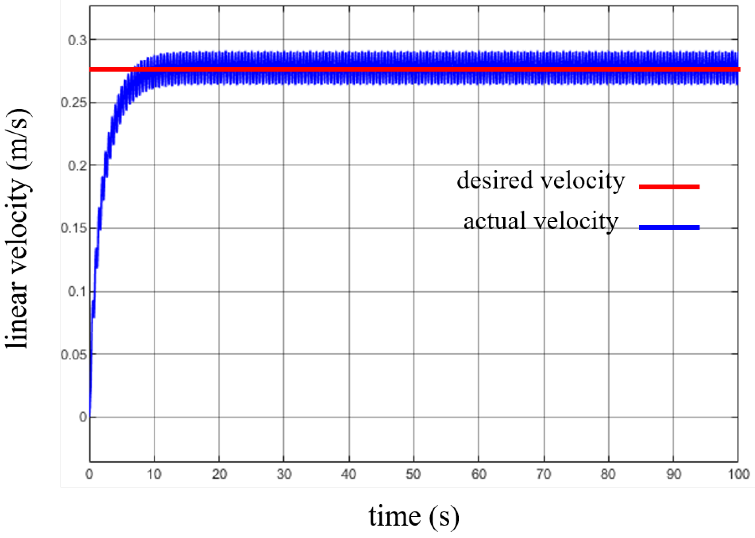
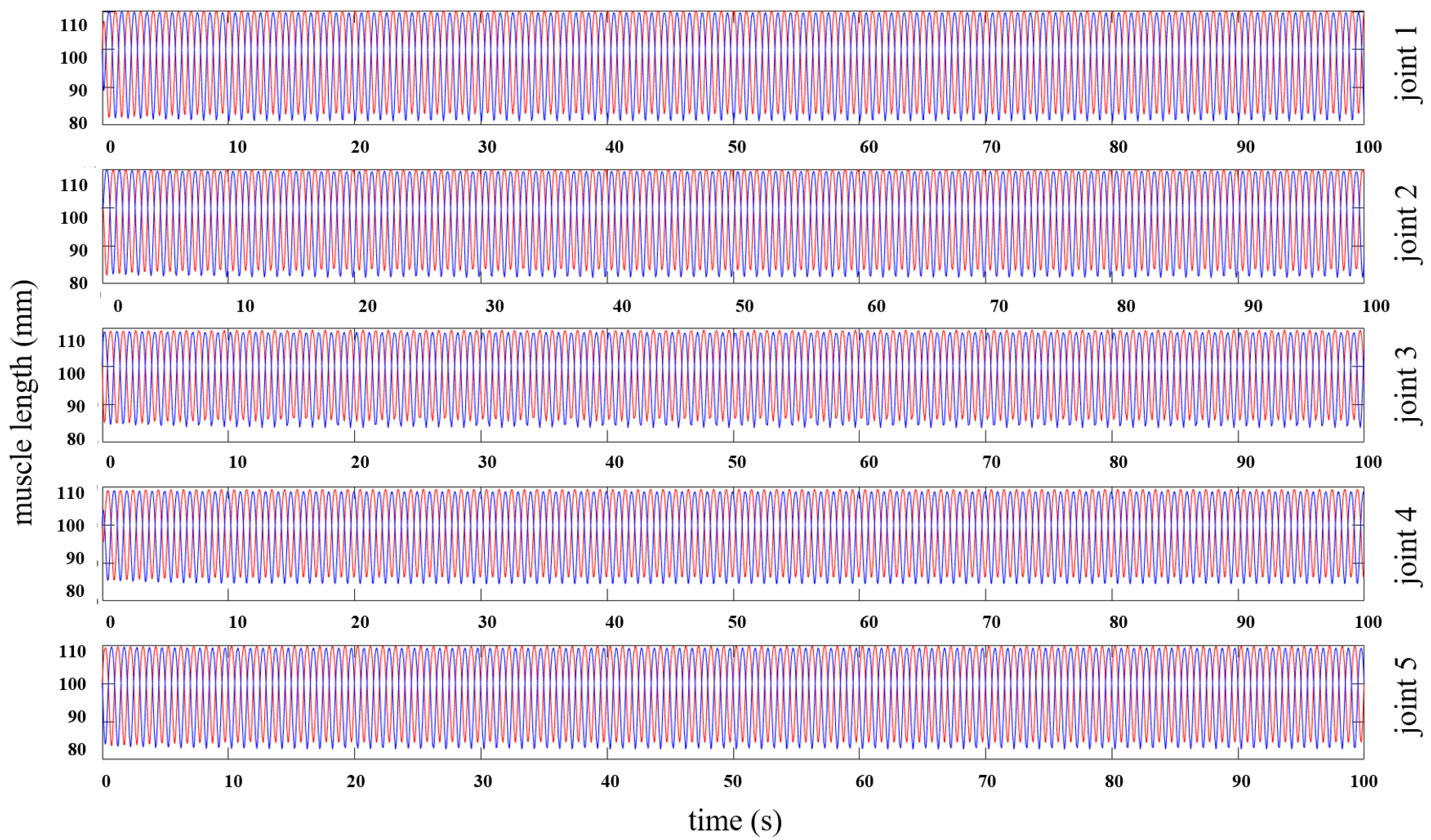
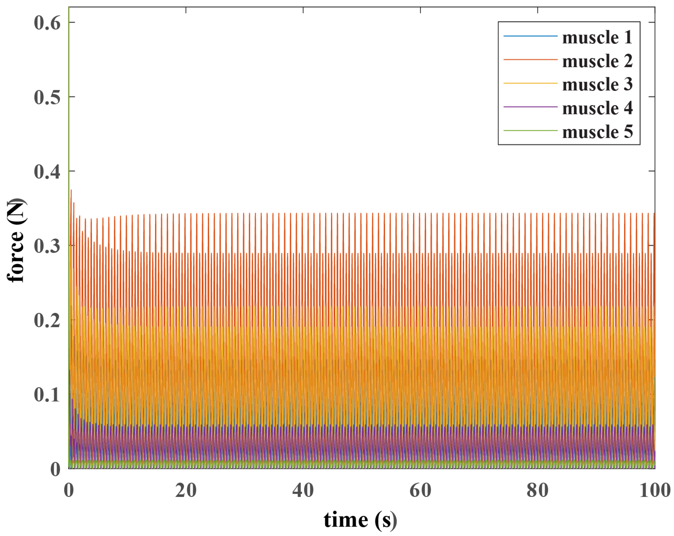
3. Results and Discussion

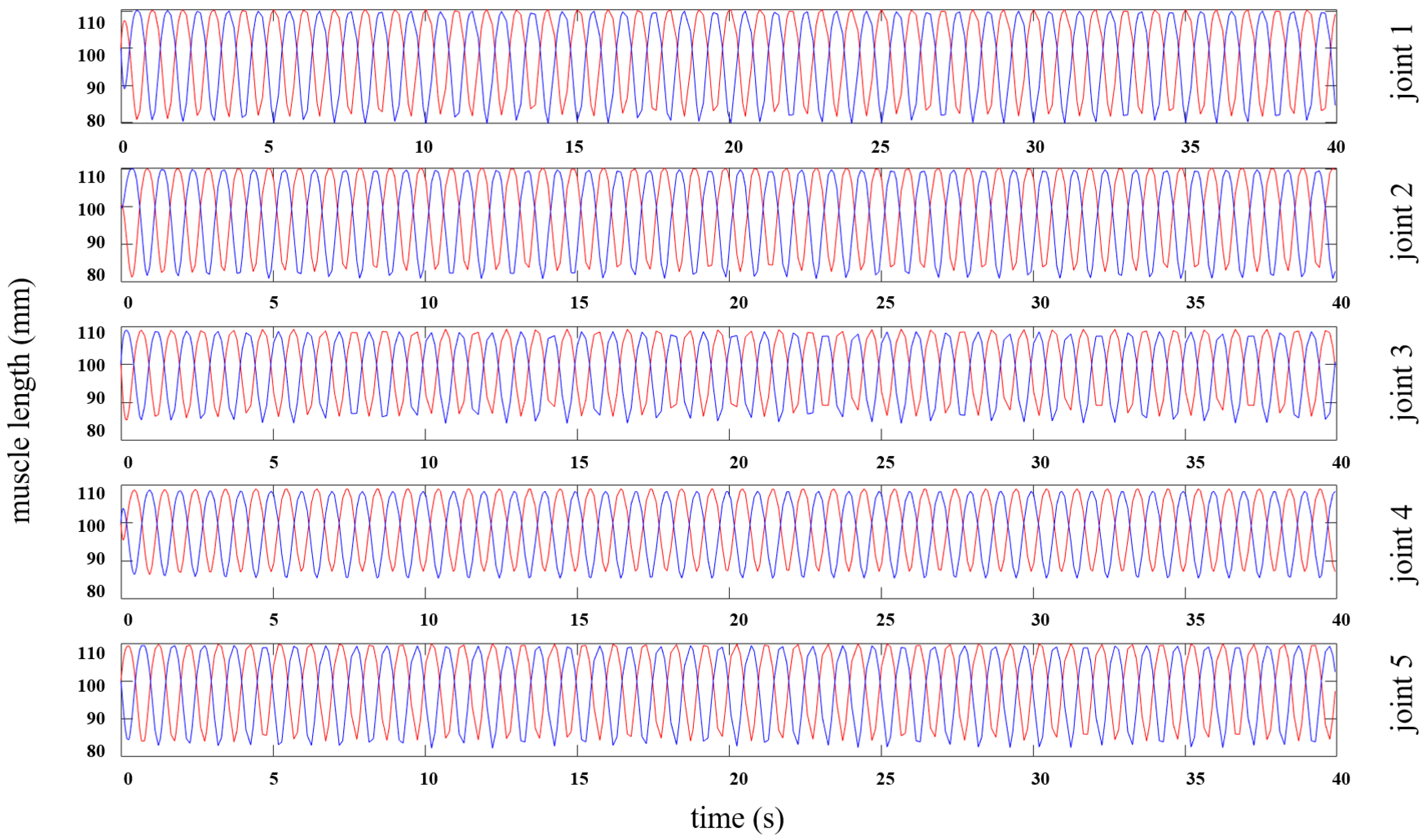
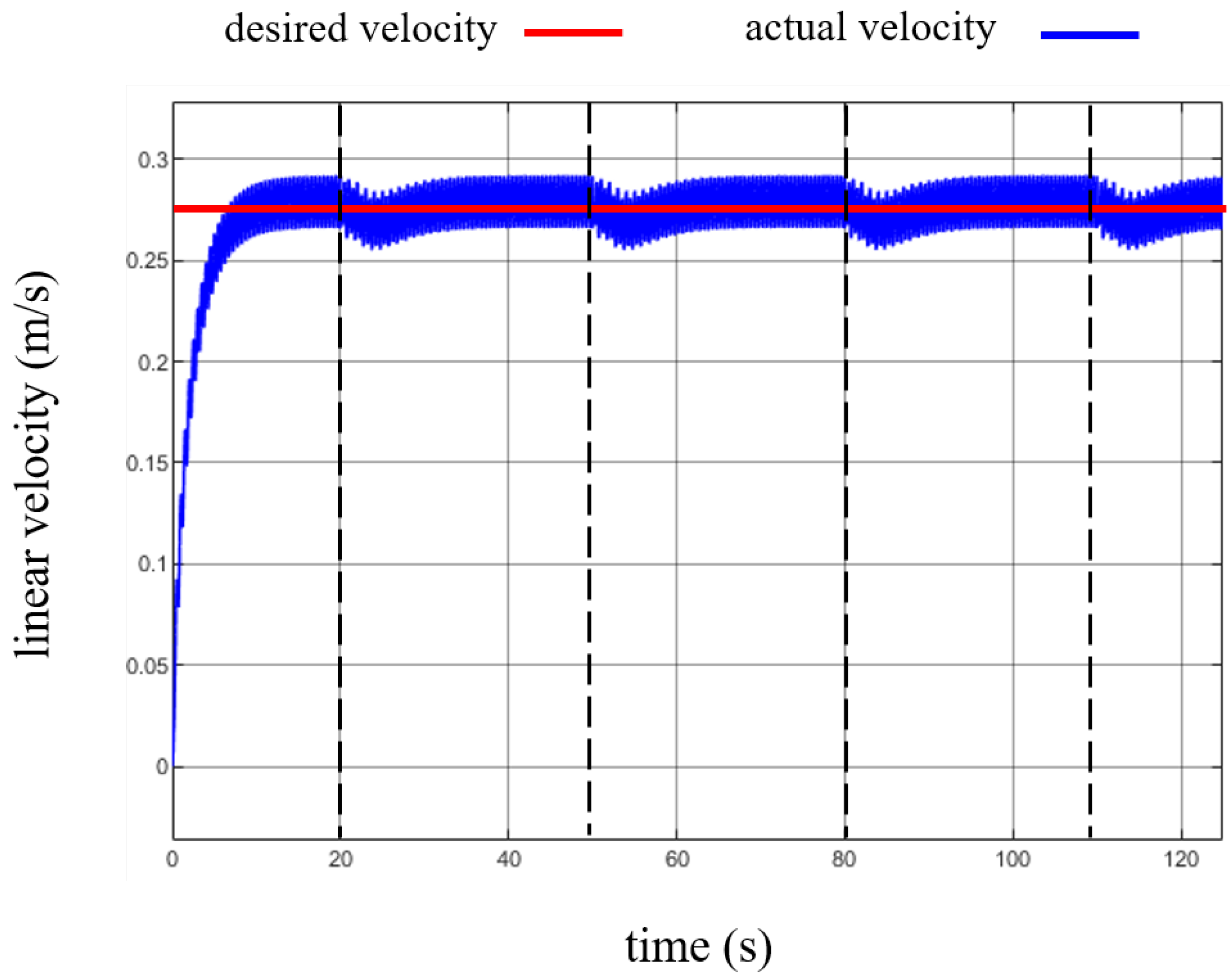
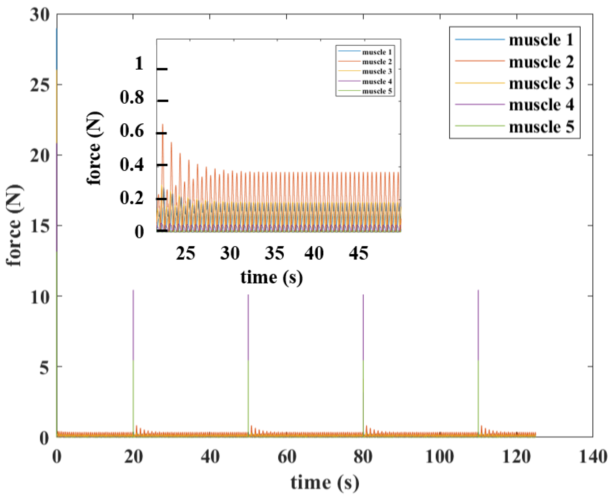
To examine the dynamic formulation and the performance of the designed controller, a series of simulation studies were conducted using a model of a six-link artificial-muscle-driven snake robot, (N = 6) with five pairs of antagonistic muscles, as shown in Figure 2. Two case studies were considered, tracking a circle-shape and a square-shape path with constant forward velocity while following the lateral undulatory gate pattern. The simulation was developed in the MATLAB environment, which ode23 was used for simulation run. The mass, length, and width of each link are set to $m=0.09$ kg, $h_1=0.1$ m, $h_2=0.05$ m, and $2w=0.05$ m, respectively. The normal and tangential friction coefficients are ${\mu }_2=0.5$ and ${\mu }_1=0.05$, respectively. The joint parameters and control gains are set as $\alpha ={30}^{\circ }$, ${\omega }_0=2\pi$ rad/s, $\beta ={72}^{\circ }$, the control gains are $k_p=1.25$, and $k_d=0.1$. The initial joint angles and velocities are set to zero. The control goal is to show that the heading direction and forward velocity tracking errors are oscillating bounded around zero, since we expect the heading and forward velocity of the robot to display oscillating behavior during undulatory locomotion [2]. On the other hand, the joint angles ${\varphi }_i$ can follow the desired sinusoidal pattern with errors exponentially approaching zero.

3.1. Circle Path

A circle-shape path with a radius of 4.2 m and a center at (1, 4.5) m was chosen in the first case. The snake robot’s head is initially located at (0, 0) with the joint angles are set to zero (i.e., a straight posture) and all linear and angular velocities are zeros. Here, we use the line-of-sight (LoS) guidance law [2] to define the heading reference angle ${\overline{\theta }}_d={tan}^{-1}\left(\frac{\overline{\mathbf{p}}}{\mathsf{\Delta }}\right)$, which will be used by the controller to adjust the snake robot’s orientation (i.e., the heading direction). The look ahead distance$\mathsf{\Delta }$ is selected as 1.5 m, which is 2.5 times of the overall length of a snake of 0.6 m, as recommended in [61]. Figure 3 shows the snapshots fo the locomotion of the snake robot following the circle path in the counterclockwise (ccw) direction. Note that the robot was initially off the path and in a stationary condition. After reaching to the desired circular path, the snake robot’s controller managed to stay on the path while finishing a full circle. The simulation time was adjusted to 100 s to ensure a full cycle of rotation, as shown in Figure 3.

The linear forward velocity of the snake robot for the first 40 seconds of the simulated-time is shown in Figure 4. The results for the full length of simulation time are shown in Figure A1. The desired value is set to a constant value of 0.275 m/s. The result demonstrate that the controller was able to approach the desire velocity in a transition time (10–90% rise-time) of about 5 s and oscillating bounded around the desired velocity with maximum and minimum velocities of 0.29 m/s and 0.264 m/s, respectively, and an amplitude of 0.013 m/s with an average velocity of approximately 0.277 m/s.

The variation of the muscle’s length over the period of 40 s of the simulated-time are illustrated in Figure 5. The relax length of each muscle is 100 mm. The PAMs are alternately activated, which contracts due to applying pressurized air, in a cyclic pattern according to the lateral undulatory gait pattern tracking the desired path in Cartesian space. The full length of simulation results are shown in Figure A1.

The range of variation of the muscles’ length are presented in the

Table 1. Maximum and minimum values of each artificial muscle length (in mm) during the simulation.

m1 Right	m1 Left	m2 Right	m2 Left	m3 Right	m3 Left	m4 Right	m4 Left	m5 Right	m5 Left
82	81	82.2	81.6	85	83.8	85.4	84.5	83.6	82.7
110.3	110	110.1	109.9	109.5	109.1	109.3	109.0	109.8	109.6

. The overall results are in the feasible range of contraction length of the PAMs.

The computed-muscle–force controller determined the required force to be generated by the PAMs, which then was transformed into the controlled pressure based on the force–length–pressure predictive model developed in our previous study [59]. The control inputs (i.e., the muscle forces) for the first 40 s of the simulated-time are shown in Figure 6. The results demonstrate a low level of force required overall to follow the circle-shape path. There is an extra effort at the beginning of the simulation due to move the snake robot from a stationary position and off the desired path. The full length of simulation results are shown in Figure A3.

3.2. Square Path

Performance of the controller is examined following a square-shape path with a constant forward velocity (0.275 m/s). The expectation was that the right-angle corners of the path would be a good challenging examination for the controller and locomotion of the snake robot. The square was considered with a side size of 8.8 m located as shown in Figure 7. The snapshots of locomotion of the muscle-driven snake robot following the path are demonstrated in Figure 7.

Similar LoS guidance law with the same look ahead distance of 1.5 m was employed in this case and the controller was able to keep the snake robot on track for most part of the path. There is a deviation with a maximum error of about 0.9 m around the corner due to the gradual adjustment of the reference heading direction ${\overline{\theta }}_d$ determined by the LoS and the constant desired velocity. The error could be reduced by adjusting the look ahead distance in the LoS guidance law and using a variable/adaptive linear velocity reference input rather than a constant value. The simulation time was adjusted in order for the snake robot to complete a full cycle in the CCW direction.

The results of the actual linear forward velocity of the snake robot against the desired constant velocity are shown in Figure 8. Although the overall response of the system demonstrate that the controller was able to control the snake robot’s forward velocity to exponentially approach the desired value in about 5 s in transition time and after then it stays bounded, oscillating around the desired value (with maximum and minimum values of 0.292 m/s and 0.268 m/s, respectively, due to an amplitude of 0.014 m/s with an average of approximately 0.28 m/s), but there are some small deviations (i.e., the average of the oscillating velocity is decreasing with the maximum error of 0.003 m/s) and rebounding behaviors corresponding to the turning motion of the snake robot passing through the corners. Similar to the circle-shape path, the actual forward velocity is oscillating bounded about the desired value.

The variation of the muscle’s length over the period of simulation time are illustrated in Figure 9. The relax length of each muscle is 100 mm. The PAMs are alternately activated, contracts due to applying pressurized air, in a cyclic pattern according to the lateral undulatory gait pattern and tracking the desired path in Cartesian space.

The range of variation of the muscles’ length are presented in the

Table 2. Maximum and minimum values of each artificial muscle length (in mm).

m1 Right	m1 Left	m2 Right	m2 Left	m3 Right	m3 Left	m4 Right	m4 Left	m5 Right	m5 Left
80.6	76	81.8	75.2	85.4	79.1	86.4	80.4	83.2	77.4
11.2	110.4	111.3	110.1	110.7	109.0	110.4	108.6	111	109.7

. However, the range of the length variation is slightly larger than the circle-shape path but the results are still in the feasible range of contraction length of the PAMs. A part of the results are magnified for better readability of the results.

The control inputs (i.e., the muscle forces) are shown in Figure 10 determined by the computed-muscle–force controller. The results demonstrated a low level of force (0.2 N to 0.6 N) required overall to follow the square-shape path. There are instances corresponding to the robot’s motion around the corners that require forces in the order of magnitude of 10 N.

4. Conclusions

This work presents the mathematical formulation for the kinematics and dynamics of a planar artificial-muscle-driven snake robot with respect to the muscles’ motion and force. The Lagrangian mechanics was employed to derive the equations of motion with muscle forces as inputs to the dynamical system. A model-based computed muscle–force–controller was designed to facilitate the tracking of the desired paths with different geometrical and topological features in the Cartesian space while generating a lateral undulation gate in the body joint space. Feedback linearization was utilized based on a change of coordinate to derive an equivalent linear input-to-state system. Next, a full state-feedback control law was designed, which satisfies the asymptotic stability of the snake robot in tracking desired trajectories. Simulation studies were carried in MATLAB on a model of a six-link snake robot. The performance of the dynamic model and the controller were successfully demonstrated in simulation studies for tracking a circle-shape path and a square-shape path with a constant linear velocity, while generating the lateral undulation gait. The results indicate a low magnitude of tracking errors, where the controlled muscle force are bounded to the actual pneumatic artificial muscles’ limitations. In future work, we will experimentally test and validate the computed muscle–force control implemented in our prototype.

References

1. Hirose, S. Biologically Inspired Robots: Snake-like Locomotors and Manipulators; Oxford Science Publications; Oxford University Press: Oxford, UK, 1993; Volume 1093. [Google Scholar]
2. Pettersen, K.Y. Snake robots. Annu. Rev. Control 2017, 44, 19–44. [Google Scholar] [CrossRef]
3. Dowling, K. Limbless locomotion: Learning to crawl. In Proceedings of the 1999 IEEE International Conference on Robotics and Automation (Cat. No. 99CH36288C), Detroit, MI, USA, 10–15 May 1999; IEEE: Piscataway, NJ, USA, 1999; Volume 4, pp. 3001–3006. [Google Scholar]
4. Liljeback, P.; Pettersen, K.Y.; Stavdahl, Ø.; Gravdahl, J.T. Experimental Investigation of Obstacle-Aided Locomotion With a Snake Robot. IEEE Trans. Robot. 2011, 27, 792–800. [Google Scholar] [CrossRef] [Green Version]
5. Onal, C.D.; Rus, D. Autonomous undulatory serpentine locomotion utilizing body dynamics of a fluidic soft robot. Bioinspir. Biomim. 2013, 8, 026003. [Google Scholar] [CrossRef] [PubMed]
6. Luo, M.; Agheli, M.; Onal, C.D. Theoretical modeling and experimental analysis of a pressure-operated soft robotic snake. Soft Robot. 2014, 1, 136–146. [Google Scholar] [CrossRef]
7. Luo, M.; Pan, Y.; Skorina, E.H.; Tao, W.; Chen, F.; Ozel, S.; Onal, C.D. Slithering towards autonomy: A self-contained soft robotic snake platform with integrated curvature sensing. Bioinspir. Biomim. 2015, 10, 055001. [Google Scholar] [CrossRef] [PubMed]
8. Branyan, C.; Fleming, C.; Remaley, J.; Kothari, A.; Tumer, K.; Hatton, R.L.; Mengüç, Y. Soft snake robots: Mechanical design and geometric gait implementation. In Proceedings of the 2017 IEEE International Conference on Robotics and Biomimetics (ROBIO), Macau, China, 5–8 December 2017; pp. 282–289. [Google Scholar] [CrossRef]
9. Branyan, C.; Menğüç, Y. Soft Snake Robots: Investigating the Effects of Gait Parameters on Locomotion in Complex Terrains. In Proceedings of the 2018 IEEE/RSJ International Conference on Intelligent Robots and Systems (IROS), Madrid, Spain, 1–5 October 2018; pp. 1–9. [Google Scholar]
10. Luo, M.; Wan, Z.; Sun, Y.; Skorina, E.H.; Tao, W.; Chen, F.; Gopalka, L.; Yang, H.; Onal, C.D. Motion Planning and Iterative Learning Control of a Modular Soft Robotic Snake. Front. Robot. AI 2020, 7, 599242. [Google Scholar] [CrossRef]
11. Godage, I.S. Swimming locomotion of Soft Robotic Snakes. arXiv 2019, arXiv:1908.05250. [Google Scholar]
12. Chirikjian, G.S.; Burdick, J.W. The kinematics of hyper-redundant robot locomotion. IEEE Trans. Robot. Autom. 1995, 11, 781–793. [Google Scholar] [CrossRef] [Green Version]
13. Wright, C.; Johnson, A.; Peck, A.; McCord, Z.; Naaktgeboren, A.; Gianfortoni, P.; Gonzalez-Rivero, M.; Hatton, R.; Choset, H. Design of a modular snake robot. In Proceedings of the 2007 IEEE/RSJ International Conference on Intelligent Robots and Systems, San Diego, CA, USA, 29 October–2 November 2007; pp. 2609–2614. [Google Scholar] [CrossRef]
14. Ma, S. Analysis of snake movement forms for realization of snake-like robots. In Proceedings of the 1999 IEEE International Conference on Robotics and Automation (Cat. No. 99CH36288C), Detroit, MI, USA, 10–15 May 1999; IEEE: Piscataway, NJ, USA, 1999; Volume 4, pp. 3007–3013. [Google Scholar]
15. Saito, M.; Fukaya, M.; Iwasaki, T. Modeling, analysis, and synthesis of serpentine locomotion with a multilink robotic snake. IEEE Control Syst. Mag. 2002, 22, 64–81. [Google Scholar]
16. Tanaka, M.; Matsuno, F. Control of snake robots with switching constraints: Trajectory tracking with moving obstacle. Adv. Robot. 2014, 28, 415–429. [Google Scholar] [CrossRef]
17. Liljebäck, P.; Pettersen, K.Y.; Stavdahl, Ø.; Gravdahl, J.T. Snake Robots: Modelling, Mechatronics, and Control; Springer Science & Business Media: Berlin, Germany, 2012. [Google Scholar]
18. Haghshenas-Jaryani, M.; Vossoughi, G. Modeling and sliding mode control of a snake-like robot with holonomic constraints. In Proceedings of the 2008 IEEE International Conference on Robotics and Biomimetics, Bangkok, Thailand, 22–25 February 2009; IEEE: Piscataway, NJ, USA, 2009; pp. 454–461. [Google Scholar]
19. Haghshenas-Jaryani, M.; Vossoughi, G. Trajectory Control of Snake-Like Robots in Operational Space Using a Double Layer Sliding Mode Controller. In Proceedings of the ASME 2015 International Design Engineering Technical Conferences and Computers and Information in Engineering Conference, Boston, MA, USA, 2–5 August 2015. [Google Scholar]
20. Sevil, L.F.H.; Haghshenas-Jaryani, M. Anomaly Detection in Joint Angle Sensor of a Snake Robot. In Proceedings of the 33rd Florida Conference on Recent Advances in Robotics (FCRAR), Melbourne, FL, USA, 14–16 May 2020. [Google Scholar]
21. Haghshenas-Jaryani, M.; Sevil, H.E.; Sun, L. Navigation and Obstacle Avoidance of Snake-Robot Guided by a Co-Robot UAV Visual Servoing. In Proceedings of the ASME 2020 Dynamic Systems and Control Conference, Virtual, 5–7 October 2020. [Google Scholar] [CrossRef]
22. Haghshenas-Jaryani, M.; Sevil, H.E. Autonomous Navigation and Obstacle Avoidance of a Snake Robot with Combined Velocity-Heading Control. In Proceedings of the 2020 IEEE/RSJ International Conference on Intelligent Robots and Systems (IROS), Las Vegas, NV, USA, 10 February 2020; pp. 7507–7512. [Google Scholar] [CrossRef]
23. Haghshenas-Jaryani, M. Maneuvering Control of a Planar Snake Robot Locomotion using a Combined Heading-Velocity-Shape Strategy. In Proceedings of the ASME 2022 International Design Engineering Technical Conferences and Computers and Information in Engineering Conference (IDETC/CIE), 46th Mechanisms and Robotics Conference, St. Louis, MO, USA, 14–17 August 2022. [Google Scholar]
24. Guo, Z.; Mahadevan, L. Limbless undulatory propulsion on land. Proc. Natl. Acad. Sci. USA 2008, 105, 3179–3184. [Google Scholar] [CrossRef] [PubMed] [Green Version]
25. Guo, X.; Zhu, W.; Fang, Y. Guided Motion Planning for Snake-like Robots Based on Geometry Mechanics and HJB Equation. IEEE Trans. Ind. Electron. 2019, 66, 7120–7130. [Google Scholar] [CrossRef]
26. Ma, S.; Araya, H.; Li, L. Development of a creeping snake-robot. In Proceedings of the 2001 IEEE International Symposium on Computational Intelligence in Robotics and Automation (Cat. No. 01EX515), Banff, AB, Canada, 29 July–1 August 2001; IEEE: Piscataway, NJ, USA, 2001; pp. 77–82. [Google Scholar]
27. Xiao, X.; Cappo, E.; Zhen, W.; Dai, J.; Sun, K.; Gong, C.; Travers, M.J.; Choset, H. Locomotive reduction for snake robots. In Proceedings of the 2015 IEEE International Conference on Robotics and Automation (ICRA), Seattle, WA, USA, 26–30 May 2015; pp. 3735–3740. [Google Scholar] [CrossRef]
28. Hatton, R.L.; Choset, H. Generating gaits for snake robots: Annealed chain fitting and keyframe wave extraction. Auton. Robot. 2010, 28, 271–281. [Google Scholar] [CrossRef]
29. Ostrowski, J.; Burdick, J. Gait kinematics for a serpentine robot. In Proceedings of the IEEE International Conference on Robotics and Automation, Minneapolis, MN, USA, 22–28 April 1996; IEEE: Piscataway, NJ, USA, 1996; Volume 2, pp. 1294–1299. [Google Scholar]
30. Ishikawa, M. Iterative feedback control of snake-like robot based on principal fibre bundle modelling. Int. J. Adv. Mechatron. Syst. 2009, 1, 175–182. [Google Scholar] [CrossRef]
31. Hicks, G.; Ito, K. A method for determination of optimal gaits with application to a snake-like serial-link structure. IEEE Trans. Autom. Control 2005, 50, 1291–1306. [Google Scholar] [CrossRef]
32. Matsuno, F.; Suenaga, K. Control of redundant 3D snake robot based on kinematic model. In Proceedings of the 2003 IEEE International Conference on Robotics and Automation (Cat. No. 03CH37422), Taipei, Taiwan, 14–19 September 2003; IEEE: Piscataway, NJ, USA, 2003; Volume 2, pp. 2061–2066. [Google Scholar]
33. Mohammadi, A.; Rezapour, E.; Maggiore, M.; Pettersen, K.Y. Maneuvering control of planar snake robots using virtual holonomic constraints. IEEE Trans. Control Syst. Technol. 2015, 24, 884–899. [Google Scholar] [CrossRef] [Green Version]
34. Kohl, A.M.; Kelasidi, E.; Mohammadi, A.; Maggiore, M.; Pettersen, K.Y. Planar maneuvering control of underwater snake robots using virtual holonomic constraints. Bioinspir. Biomim. 2016, 11, 065005. [Google Scholar] [CrossRef]
35. Chang, A.H.; Hyun, N.P.; Verriest, E.I.; Vela, P.A. Optimal Trajectory Planning and Feedback Control of Lateral Undulation in Snake-Like Robots. In Proceedings of the 2018 Annual American Control Conference (ACC), Milwaukee, WI, USA, 27–29 June 2018; pp. 2114–2120. [Google Scholar] [CrossRef]
36. Mazzolai, B.; Laschi, C. A vision for future bioinspired and biohybrid robots. Sci. Robot. 2020, 5, eaba6893. [Google Scholar] [CrossRef]
37. Morimoto, Y.; Onoe, H.; Takeuchi, S. Biohybrid robot powered by an antagonistic pair of skeletal muscle tissues. Sci. Robot. 2018, 3, eaat4440. [Google Scholar] [CrossRef] [Green Version]
38. Davis, S.; Tsagarakis, N.; Canderle, J.; Caldwell, D.G. Enhanced modelling and performance in braided pneumatic muscle actuators. Int. J. Robot. Res. 2003, 22, 213–227. [Google Scholar] [CrossRef]
39. Zhang, J.; Sheng, J.; O’Neill, C.T.; Walsh, C.J.; Wood, R.J.; Ryu, J.H.; Desai, J.P.; Yip, M.C. Robotic Artificial Muscles: Current Progress and Future Perspectives. IEEE Trans. Robot. 2019, 35, 761–781. [Google Scholar] [CrossRef]
40. Schroder, J.; Erol, D.; Kawamura, K.; Dillman, R. Dynamic pneumatic actuator model for a model-based torque controller. In Proceedings of the 2003 IEEE International Symposium on Computational Intelligence in Robotics and Automation. Computational Intelligence in Robotics and Automation for the New Millennium (Cat. No. 03EX694), Kobe, Japan, 16–20 July 2003; IEEE: Piscataway, NJ, USA, 2003; Volume 1, pp. 342–347. [Google Scholar]
41. József, S.; Gábor, S.; János, G. Investigation and application of pneumatic artificial muscles. Biomech. Hung. 2010, 3, 208–214. [Google Scholar]
42. Tondu, B.; Lopez, P. Modeling and control of McKibben artificial muscle robot actuators. IEEE Control Syst. Mag. 2000, 20, 15–38. [Google Scholar]
43. Craddock, M.; Augustine, E.; Konerman, S.; Shin, M. Biorobotics: An Overview of Recent Innovations in Artificial Muscles. Actuators 2022, 11, 168. [Google Scholar] [CrossRef]
44. Antonelli, M.G.; Beomonte Zobel, P.; Durante, F.; Zeer, M. Modeling-Based EMG Signal (MBES) Classifier for Robotic Remote-Control Purposes. Actuators 2022, 11, 65. [Google Scholar] [CrossRef]
45. Balasubramanian, S.; Wei, R.; Perez, M.; Shepard, B.; Koeneman, E.; Koeneman, J.; He, J. RUPERT: An exoskeleton robot for assisting rehabilitation of arm functions. In Proceedings of the 2008 Virtual Rehabilitation, Vancouver, BC, Canada, 25–27 August 2008; IEEE: Piscataway, NJ, USA, 2008; pp. 163–167. [Google Scholar]
46. Kobayashi, H.; Hiramatsu, K. Development of muscle suit for upper limb. In Proceedings of the IEEE International Conference on Robotics and Automation, New Orleans, LA, USA, 26 April–1 May 2004; IEEE: Piscataway, NJ, USA, 2004; Volume 3, pp. 2480–2485. [Google Scholar]
47. Koeneman, E.; Schultz, R.; Wolf, S.; Herring, D.; Koeneman, J. A pneumatic muscle hand therapy device. In Proceedings of the 26th Annual International Conference of the IEEE Engineering in Medicine and Biology Society, San Francisco, CA, USA, 1–5 September 2004; IEEE: Piscataway, NJ, USA, 2004; Volume 1, pp. 2711–2713. [Google Scholar]
48. Wongsiri, S.; Laksanacharoen, S. Design and construction of an artificial limb driven by artificial muscles for amputees. In Proceedings of the International Conference on Energy and the Environment, Prince of Songkla University, Hat Yai, Songkla, Thailand, 11–12 December 2003; pp. 11–12. [Google Scholar]
49. Wehner, M.; Tolley, M.T.; Mengüç, Y.; Park, Y.L.; Mozeika, A.; Ding, Y.; Onal, C.; Shepherd, R.F.; Whitesides, G.M.; Wood, R.J. Pneumatic Energy Sources for Autonomous and Wearable Soft Robotics. Soft Robot. 2014, 1, 263–274. [Google Scholar] [CrossRef] [Green Version]
50. Gray, J. The mechanism of locomotion in snakes. J. Exp. Biol. 1946, 23, 101–120. [Google Scholar] [CrossRef]
51. Rezaei, S.M.; Barazandeh, F.; Haidarzadeh, M.S.; Sadat, S.M. The effect of snake muscular system on actuators’ torque. J. Intell. Robot. Syst. 2010, 59, 299–318. [Google Scholar] [CrossRef]
52. Jayne, B.C. Muscular mechanisms of snake locomotion: An electromyographic study of the sidewinding and concertina modes of Crotalus cerastes, Nerodia fasciata and Elaphe obsoleta. J. Exp. Biol. 1988, 140, 1–33. [Google Scholar] [CrossRef]
53. Jayne, B.C. Muscular mechanisms of snake locomotion: An electromyographic study of lateral undulation of the Florida banded water snake (Nerodia fasciata) and the yellow rat snake (Elaphe obsoleta). J. Morphol. 1988, 197, 159–181. [Google Scholar] [CrossRef]
54. Moon, B.R.; Gans, C. Kinematics, muscular activity and propulsion in gopher snakes. J. Exp. Biol. 1998, 201, 2669–2684. [Google Scholar] [CrossRef] [PubMed]
55. Wang, T.; Wang, Z.; Wu, G.; Lei, L.; Zhao, B.; Zhang, P.; Shang, P. Design and Analysis of a Snake-like Surgical Robot with Continuum Joints. In Proceedings of the 2020 5th International Conference on Advanced Robotics and Mechatronics (ICARM), Shenzhen, China, 18–21 December 2020. [Google Scholar] [CrossRef]
56. Granosik, G.; Borenstein, J. Integrated joint actuator for serpentine robots. IEEE/ASME Trans. Mechatron. 2005, 10, 473–481. [Google Scholar] [CrossRef]
57. Kakogawa, A.; Jeon, S.; Ma, S. Stiffness design of a resonance-based planar snake robot with parallel elastic actuators. IEEE Robot. Autom. Lett. 2018, 3, 1284–1291. [Google Scholar] [CrossRef]
58. Ute, J.; Ono, K. Fast and efficient locomotion of a snake robot based on self-excitation principle. In Proceedings of the 7th International Workshop on Advanced Motion Control. Proceedings (Cat. No. 02TH8623), Maribor, Slovenia, 3–5 July 2002; IEEE: Piscataway, NJ, USA, 2002; pp. 532–539. [Google Scholar]
59. Lopez, M.; Haghshenas-Jaryani, M. A Muscle-Driven Mechanism for Locomotion of Snake-Robots. Automation 2022, 3, 1–26. [Google Scholar] [CrossRef]
60. Lanczos, C. The Variational Principles of Mechanics; Courier Corporation: Chelmsford, MA, USA, 2012. [Google Scholar]
61. Fossen, T.I. Handbook of Marine Craft Hydrodynamics and Motion Control; John Wiley & Sons: Hoboken, NJ, USA, 2011. [Google Scholar]
Figure 1. Schematic of the artificial-muscle-driven snake robot kinematics, (a) geometry of the mechanism and (b) kinematics of the muscle length and the joint angle, and (c) the free body diagram of a module of the snake robot including the forces acting on the body of the snake robot.
Actuators 11 00194 g001
Figure 2. Overall kinematics of a snake robot modeled as an articulated body with N moving links and N joints.
Actuators 11 00194 g002
Figure 3. Snapshots of locomotion of the snake robot following a circle path.
Actuators 11 00194 g003
Figure 4. Forward velocity of the snake robot following a circle path.
Actuators 11 00194 g004
Figure 5. Time evolution of muscles’ length of the snake robot following a circle path. The blue and red colors are the length of the left and right muscles at each joint, respectively.
Actuators 11 00194 g005
Figure 6. Muscles’ force of the snake robot following a circle path.
Actuators 11 00194 g006
Figure 7. Snapshots of the snake robot’s locomotion following a square path.
Actuators 11 00194 g007
Figure 8. Forward velocity of the snake robot following a square-shape path.
Actuators 11 00194 g008
Figure 9. Muscles’ length of the snake robot following a square path.
Actuators 11 00194 g009
Figure 10. Muscles’ force of the snake robot following a square-shape path with a zoom-in box for a part of the result.
Actuators 11 00194 g010