Abstract
The surging popularity of adopting industrial robots in smart manufacturing has led to an increasing trend in the simultaneous improvement of the energy costs and operational efficiency of motion trajectory. Motivated by this, multi-objective trajectory planning subject to kinematic and dynamic constraints at multiple levels has been considered as a promising paradigm to achieve the improvement. However, most existing model-based multi-objective optimization algorithms tend to come out with infeasible solutions, which results in non-zero initial and final acceleration. Popular commercial software toolkits applied to solve multi-objective optimization problems in actual situations are mostly based on the fussy conversion of the original objective and constraints into strict convex functions or linear functions, which could induce a failure of duality and obtain results exceeding limits. To address the problem, this paper proposes a time-energy optimization model in a phase plane based on the Riemann approximation method and a solution scheme using an iterative learning algorithm with neural networks. We present forward-substitution interpolation functions as basic functions to calculate indirect kinematic and dynamic expressions introduced in a discrete optimization model with coupled constraints. Moreover, we develop a solution scheme of the complex trajectory optimization problem based on artificial neural networks to generate candidate solutions for each iteration without any conversion into a strict convex function, until minimum optimization objectives are achieved. Experiments were carried out to verify the effectiveness of the proposed optimization solution scheme by comparing it with state-of-the-art trajectory optimization methods using Yalmip software. The proposed method was observed to improve the acceleration control performance of the solved robot trajectory by reducing accelerations exceeding values of joints 2, 3 and 5 by 3.277 rad/s2, 26.674 rad/s2, and 7.620 rad/s2, respectively.
1. Introduction
As industrial robots are applied in more and more manufacturing scenarios, high efficiency and low energy cost of the motion trajectory are essential to meet the production needs and reduce resource consumption [1,2,3]. Time-energy cost-optimal trajectory planning for robots given a task path is conducted while surrendering limitations of kinematic and dynamic capabilities for safe operation. Effective trajectory optimization resolution of redundant robots with compliance to single-level physical constraints, such as velocity, is easy to implement. However, existing model-based algorithms for robot path planning may result in joint-angle drift and non-zero final joint velocity and acceleration when systems are subjected to comprehensive velocity, acceleration and torque constraints and controlled at multiple levels, as discussed in [4,5,6].
Recently, many kinds of solver software, combined with various optimization methods, have been utilized in robot planning research to avoid obtaining infeasible solutions. The objective and constraints input into solver software should follow the specified rules of optimization theories, such as convex optimization (CO), linear programming (LP) [7], quadratic programming (QP) [5], second-order cone programming (SOCP) [3], concave-convex procedure (CCCP) [8], and semi-definite programming (SDP). Each algorithm of the aforementioned software toolkits has its strict solution form and is usually solved by Lagrange duality and the interior point method [9], also known as the barrier method or combined methods. Moreover, the solving process of the above software is implicit, which is not conducive to estimating a global optimum or local minima. Thus, for the trajectory optimization problem of robots with precise multi-level constraints, it is necessary to establish a generalized time-energy consumption optimization model and to develop algorithms with feasible solutions in actual scenes.
To address the issues, this paper proposes a novel multi-objective trajectory optimization approach with the goal of simultaneously minimizing the time and energy consumption of industrial robots. First, we formulate the optimization problem by establishing the weighting function of time and energy consumption in generalized path coordinates. The transformed trajectory variables in the weighting function corresponding to the angle, velocity and acceleration in joint coordinates are considered as generated optimizing variables. Then, we present forward-substitution interpolation functions as basic functions to calculate indirect velocity and acceleration expressions introduced in the discrete optimization model and obtain segmented smooth paths in terms of trajectory variables. Consequently, we impose an iterative metaheuristic scheme to solve trajectory variables in the complex optimization problem based on artificial neural networks, avoiding the fussy conversion of strict convex or linear functions. Moreover, velocity, acceleration and torque constraints controlled in joint performance parameter limits in the overall process of motion are also the focus of the trajectory design and optimization in this paper, according to the actual needs of industrial robots. The proposed trajectory optimization model can adjust the variable values according to the requirement of high-speed motion or low energy consumption. Finally, extensive experiments are conducted to verify the effectiveness of the proposed optimization solution scheme by comparing it with the state-of-the-art trajectory optimization methods using Yalmip software.
2. Related Work
Generally, to solve a trajectory planning problem, joint angles of an industrial robot, given the desired path described in Cartesian space, are first calculated by an inverse kinematic model. Then, trajectory variables, including velocity and acceleration as functions of angle derivative in terms of time, are optimized to achieve the minimum running time or energy consumption with the demands of multi-level control for safe operation. Feng et al. [10] employed fifth-order polynomial expressions to construct joint trajectories and established a time-energy consumption optimization model by introducing velocity variables obtained from the pre-defined trajectory. Since an industrial robot usually has six joints, the optimization objective of all joint angles is a multidimensional expression. For simplification of the objective function, Palleschi et al. [11] described path coordinates as a normalized trajectory variable based on phase plane theory to reduce the high-dimensional state space and solve the tracking problem of a minimum-time path with smooth and continuous accelerations by the SCIP solver of Opti Toolbox. Although software can generate a set of optimized solutions, the implicit solving process is often difficult to converge when multi-level constraints of the robot are required to be controlled.
For the control of robots with optimal trajectory under the multi-level constraints enforced, a conventional solution is the Jacobian pseudo-inverse method, which can be regarded as an analytical solution with a direct correlation between end-effector and joint trajectory variables. Ramezani and Williams [12] present an optimal redundancy resolution technique by using the augmented Jacobian to provide feasible solutions for the minimum objective function. The traditional Jacobian pseudo-inverse scheme is just applicable to trajectory optimization with joint physical limits expressed as equality equations, while inequality constraints can hardly be introduced to this direct solution scheme.
To achieve efficient redundancy resolution for multi-level control of a robot’s trajectory, Verscheure et al. [3] transformed the optimization model with consideration of time, energy cost and smoothness into a convex optimization problem, and presented a transcription method to solve a SOCP with inequality constraints using robust numerical algorithms in Yalmip. Nagy and Vajk [7] converted a profile generation model into linear programming (LP) form and solved it with a sequential optimization method. Steinhauser and Swevers [4] presented a two-step iterative learning algorithm that compensates for inevitable model-plant mismatch of time-optimal motion, which improved tracking performance and ensured feasibility based on a sequential convex log barrier method. Zhang et al. [6] formulated the trajectory resolution problem subject to joint angle, velocity, and acceleration constraints as a QP to overcome computationally intensive pseudo-inverse-based schemes. The optimization models referred to require the objective and constraints to be converted to satisfy the strict solving forms, which sometimes induces a failure of duality and obtains results exceeding limits.
Among optimization approaches, metaheuristic algorithms have shown their capabilities for searching for near-global-optimal solutions to numerical real-valued test problems, such as the genetic algorithm (GA) [13,14], particle swarm optimization (PSO) [15], artificial neural networks (ANNs) [16,17], and so forth. Chen et al. [5] formulated a multi-level simultaneous minimization scheme as a dynamical quadratic program (DQP), which was solved by a piecewise linear projection equation neural network. Abu-Dakka et al. [14] constructed smooth joint trajectories with cubic polynomial functions as basic functions in a segmented path to establish an optimization model of minimum time, energy and jerk. Undetermined parameters in basic functions were solved by a parallel-populations genetic algorithm (PPGA) procedure. Based on the multi-objective genetic optimization algorithm NSGA-II, Shi et al. [18] solved the optimization problem in the multi-objective form.
Although the above state-of-the-art metaheuristic algorithms have good effects on solving general optimization problems, some of these methods applied in trajectory planning cannot guarantee the initial and final zero-velocity and zero-acceleration and joint-angle drift sometimes occurs, so are not suitable for actual conditions of the robot operation. In addition to the solution algorithm, the established trajectory optimization model and the form of internal basic function for iteration calculation, dynamic equation expressions, and other factors will also have an impact on the output trajectories results. Thus, it is necessary to establish a multi-objective optimization model with consideration of the applicable conditions in the actual situation.
3. Robot Kinematics and Dynamics Modeling
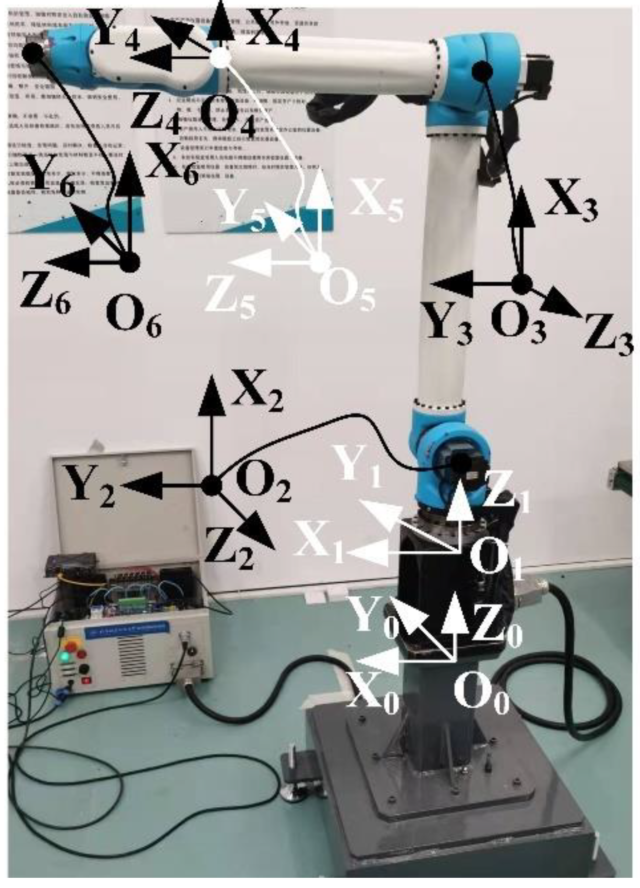
In this paper, a serial 6-axis robot is considered to establish the time-energy optimization model, the structure of which is shown in Figure 1. The modified Denavit–Hartenberg (MDH) parameters are presented in Table 1. Forward and inverse kinematic models of the specified robot can be established with these parameters.

Figure 1.
Specified robot structure.

Table 1.
Modified Denavit–Hartenberg parameters of the specified robot.
Dynamic equations of the robot with several identified parameters are established to express the joint torques according to the iterative Newton-Euler formulation [19]. To establish an accurate dynamic identification model, inertia terms and friction terms are introduced in the torques expressions [20] as follows:
where and denote the velocity and acceleration of joint i, is the inertia moment for rotor and gears of actuator i, and are the viscous and Coulomb friction coefficients. It should be noted that the inertia tensor related to the center of mass of link in should be converted in terms of the inertia tensor related to the origin of the joint coordinate by introducing the expression
where , is the mass of link i, is the identity matrix, the undetermined vector locates the center of mass of link i relative to the coordinate system {Oi}. The vector of the identified parameters for each joint torque is denoted as
which contains position coordinate components of the center of mass of link (, , ), inertia moment components of link i (, , , , , ).
The differential Equation (1) in terms of 78 dynamic parameters can be linearized and expressed by
where is the joint torques vector, is the standard parameters vector, is a 6 × 78 regressor matrix and q is the joint position vector. The above equation can be transformed into a simplified form with a minimal set of 52 identifiable parameters by regrouping the original parameters , a detailed derivation process for which can be seen in [21,22]. Thus, the torque can be simplified as
where is a subset of the independent columns of . We sample several data of torques and joint angles when the robot moves according to an exciting trajectory at , and over-determined linear equations are obtained as
where observation matrix is , the torques vector is , and is a vector of sampling error. Based on the least square method, the minimum identification parameters set can be obtained by
The calculated minimum set of combined parameters is listed in Table A1 in Appendix A. The dynamic model with an iterative Newton–Euler formulation is obtained by substituting into Equation (1).
Then, we rewrite the dynamic model into the state-space equation form, as follows:
where is the mass or inertia matrix, is the vector of Coriolis and centrifugal terms, is the vector of gravity terms, and is the vector of friction terms.
4. Problem Formulation
This section formulates the time-energy optimal trajectory planning problem of a robot with precise multi-level constraints. The optimization objective and complex constraints, including velocity, acceleration and torque, are derived based on the phase plane theory and Riemann approximation method. For effective numerical computing, the optimization model introduces the discrete kinematic and dynamic equation results.
4.1. Original Formulation
Minimizing the total motion time of an industrial robot is simply expressed as . For optimization of the energy cost, the main resistance energy consumption of the servo circuit in each robot joint is modeled by Joule’s law, as follows:
where is electric current and is the resistance. Due to the relevant relations between torque and current, the above equation can be proportional to the expression in terms of torque:
For a single servo motor system, the energy consumption model during the running time should be:
which omits the coefficient since it is constant for one joint. Then, energy consumption is also proportional to the integral of the torque square . Total energy consumption of a robot can be optimized by minimizing the normalized expression:
which divides the square of maximum torque limit for equalized optimization of every joint energy.
For simultaneous minimizing of the time and energy of a robot with multi-level constraints, the following synthetical optimization model is established as
Subjected to
where is the weight coefficient; overline and underline of velocity, acceleration and torque represent the maximum and minimum values.
4.2. Reformulation Based on Phase Plane Theory
Due to the complexity of the multidimensional-optimal problem for an industrial robot with six joints, the optimization objective is calculated using six different trajectories functions until the minimum operation time value for any of all joints is found. For simplification of the objective function, we describe path coordinates as a parameterized trajectory variable based on phase plane theory to reduce the high-dimensional state space to one dimension.
Based on the Pontryagin principle [23], the optimization independent variable t can be replaced by the trip proportion variable assigned to the path curve through a generalized coordinate transformation . Then, the reformulated optimization problem is analyzed in the S-phase plane. Joint position q is a function of s, notated as . Joint velocity and acceleration are transformed as
where , , is defined as , . Moreover, substituting the relations (15) into the dynamic equation (8), yields
where the term is linear to the joint velocity [24], which can be described as . Meanwhile, the trajectory velocity is positive when the robot runs along a path, such that the sign function of is equal to . We define , , and for simplification of Equation (16).
The normalized time-energy consumption optimization model for the robot trajectory is reformulated by substituting expression (16) and as
where represents .
Since the integral optimization model is difficult to be solved, it is converted to discrete sums based on the Riemann approximation method. Then, the corresponding discretization and normalization are carried out for the time-energy optimization objective with multi-level constraints, as follows:
where is the j-th point proportion of the divided path curve, . Simultaneously, velocity and acceleration in joint coordinate and torque constraints are discrete as
where , for j = 1, …, n − 1 is assumed as a piecewise function. In the case of the dramatic increase in velocity and acceleration, the corresponding constraints are limited in the range of 1/(n − 1) multiple maximum values at the initial and final interval segments.
5. Solution Algorithm
In this section, we present a solving scheme of a time-energy optimal trajectory with a forward-substitution interpolation method and metaheuristic algorithm. Firstly, high-order polynomial interpolation functions are applied as basic functions to calculate indirect kinematic and dynamic expressions introduced in a discrete optimization model and other constraints. Then, we develop a solution algorithm based on artificial neural networks to generate candidate solutions for each iteration without any conversion into strict forms, until a minimum objective function value is achieved.
5.1. Forward-Substitution Interpolation Basic Functions
A path that a robot usually moves around is specified by a series of space position coordinates . Geometric curve functions, such as the cubic Bezier or B-spline curve, could be used to fit these points, as
where control points ,. Then the interpolated path points , , … coordinates are calculated by the cubic Bezier curve function, and we add the number of path points to N. For convenience, we notate points as , , …, ,…, . Although the partitioned Bezier curve function describes the discrete interpolated points space coordinates between the specified points along the path. Each joint positions vector in the joint coordinate system corresponding to the path point can be resolved by the inverse kinematic model with position coordinate and specified pose orientation vector, as rotations around the x-axis, y-axis, z-axis .
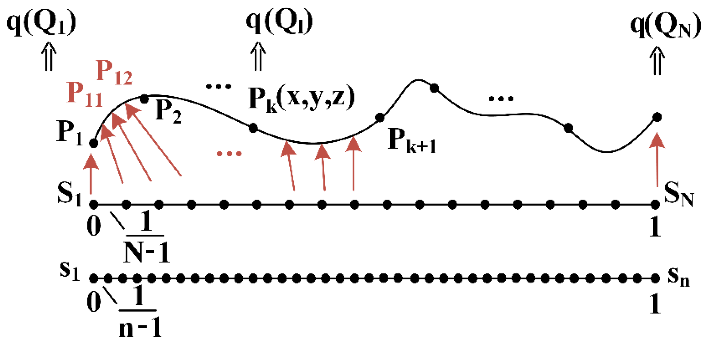
To express the joint trajectory function, isometric distributed generalized path curve parameters ,…, are introduced to establish the mapping relation of unevenly distributed trajectory points ,…, . Figure 2 shows the correspondence relations diagram of path points and generalized path curve parameters. Due to the velocity and acceleration requirements, the third-order polynomial function is the lowest order form we choose to be an interpolated trajectory function in terms of the curve parameter S. Moreover, the initial and final trajectory functions with zero-velocity and zero-acceleration are considered by applying the fifth-order polynomial function. The common fitting method of the fixed segmentation function just uses joint angles of two adjacent points, such as and , to establish the trajectory function. In this case, the higher derivatives of the adjacent trajectory functions have saltation at the connecting point. To solve this problem, we propose a forward-substitution interpolation as a predefined basic trajectory function expressed as
where , , , , , , , , , , and are the polynomial coefficients, d is the nearest integer less than or equal to 0.1(N − 1), and half of the added continuous selected points number is decided by the set variation value. Quantity l increases until the root mean squared error of the left-fitting value and the right-truth value of Equations (21)–(23) are larger than the set variation value. The super-positive definite Equations (21)–(23) are solved by the least square method.

Figure 2.
Correspondence relations diagram of path points and generalized path curve parameters.
When the path curve proportion variable s chosen is different from the generalized path curve parameter S, we just need to determine which segment s belongs to. The trajectory function and derivative and are substituted into the indirect kinematic and dynamic expressions , , in the discrete optimization objective expression (17) and constraints Equation (18).
5.2. Dynamic Metaheuristic Optimization Algorithm
After the pre-defined value , and is substituted, the discrete optimization objective is a function in terms of variables . The sum terms of a normalized torque square in objective expression (17) will induce high-order nonlinear forms of independent variables , which is difficult to be solved by the model-based analytical optimization algorithm or solver software without any conversion. Thus, we develop a solution algorithm based on artificial neural networks (ANN) [17] to handle this issue.
In an n-dimensional optimization problem, a pattern solution representing input data in the ANN, is defined as
First, a starting candidate of the pattern solution matrix H is generated, which is randomly generated between the lower and upper bounds of a problem:
Cost functions corresponding to pattern solutions are obtained by
where f is the objective function in expression (17).
The candidate solution with the minimum objective function value for all pattern solutions is selected as the target solution. This target solution will be updated at each iteration. After determining the target solution among the other pattern solutions, the target weight , corresponding to the target solution, must be selected from the population of weight (weight matrix) by the following expression:
where is a matrix generating random numbers uniformly between zero to one during iterations, and is an iteration index. The weight superscript relates to its pattern solution (e.g., is related to the second pattern solution) and the weight subscript is shared with the other pattern solutions (e.g., is shared with the third pattern solution). Every pattern solution has its corresponding weight value which has been involved in generating a new candidate solution. Moreover, the sum of elements in is 1. After forming , new pattern solutions are generated by the following expression:
Therefore, the new pattern solution has been updated for iteration . Based on the best weight value called “target weight”, the weight matrix should be updated, as follows:
where is a uniformly distributed random number in the range [0, 1].
In ANN, the bias current is introduced, of which the bias operator modifies a certain percentage of the pattern solutions in the new population of pattern solutions and updated weight matrix . The bias operator in the ANN is another way to explore the search space, which prevents the algorithm from premature convergence and modifies individual numbers in the population. In fact, the bias operation acts as noise to the new pattern solutions and the updated weight matrix.
Then new pattern solutions in the population from their current positions in the search space are transferred to new positions to update and generate better quality solutions toward the target solution by the transfer function operator. The transfer function (TF) operation is defined by the following equation:
where the i-th new pattern solution is transferred to the updated position .
In summary, the optimization problem can be solved by the general behavior of ANN, which can be described by
where and are the next and current locations of pattern solution i-th, respectively. is a population of pattern solutions with updated weights.
6. Results and Discussion
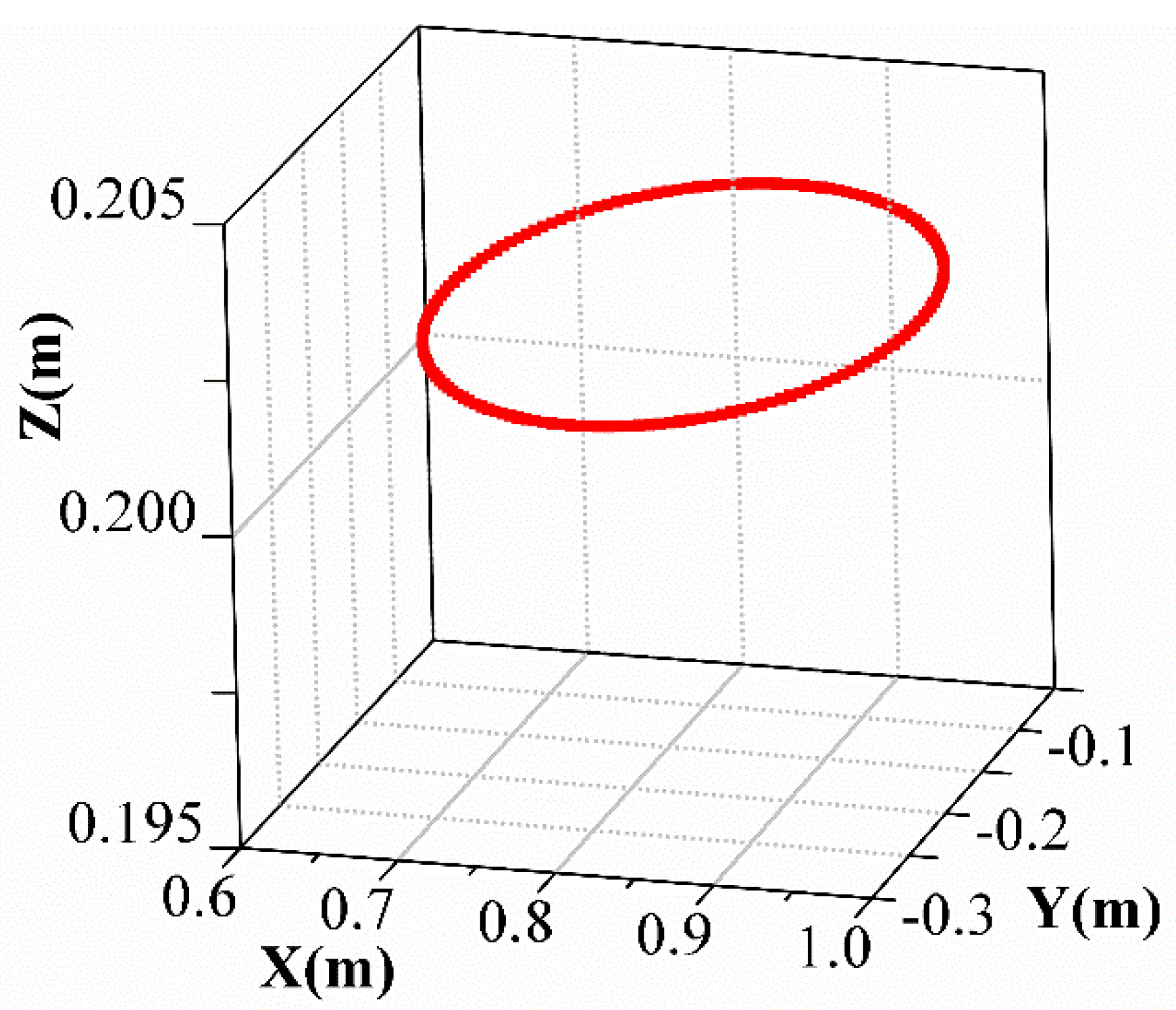
To assess the general applicability and verify the accuracy of the proposed method, optimal time trajectory and time-energy synthesis optimization results were calculated using simulation and actual experiments with the kinematic and dynamic boundary conditions compared with the state-of-the-art algorithms in [3] using Yalmip software. The boundary conditions are listed in Table 2. A circle path of robot motion was applied to test the effectiveness of the proposed method, as shown in Figure 3. The original coordinates values of the robot end were (0.805133 m, −0.328446 m, 0.201903 m), and the radius of the circle was 0.15 m. The orientations of the robot end in Cartesian space were (3.137975 rad, −0.015916 rad, 1.620108 rad).
Table 2.
Absolute value limits of joint angles, velocities and accelerations.
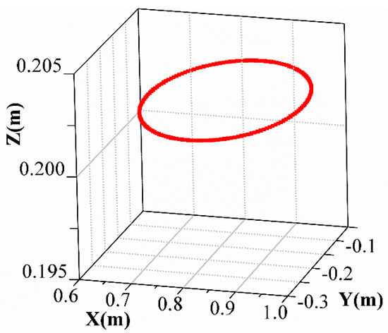
Figure 3.
A circle path of robot motion.
In [3], the minimum objective (17) is solved by the conventional optimization method SOCP, which converts the non-convex function into convex form with additional constraint conditions, as follows:
The above fussy conversion of strictly convex functions is avoided by the proposedThe above fussy conversion of strictly convex functions is avoided by the proposed optimization model directly solved by the ANN algorithm in Section 5. Moreover, the second-order polynomial interpolation functions are applied as basic functions to calculate indirect kinematic and dynamic expressions introduced in a discrete optimization model and other constraints in reference [3].
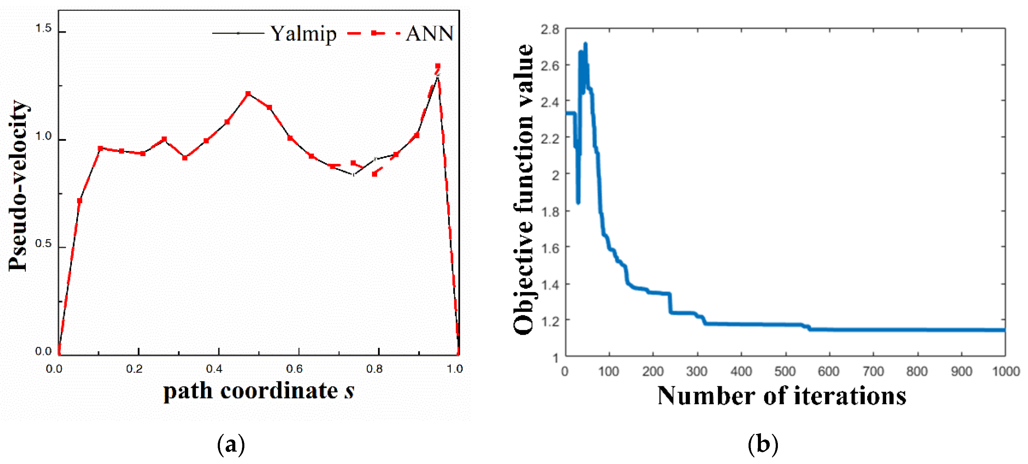
For verification of the accuracy and efficiency of the proposed method, the optimization variable results in objective function solved by SDPT3 optimization toolkit in Yalmip and the ANN algorithm, when the basic functions are the second-order polynomial interpolation functions and the initial and final velocity and acceleration boundaries are neglected as in [3], as shown in Figure 4. We select discrete points when the number of s is 20. As can be seen in Figure 4, optimization variable h(sj) values at different coordinates solved by the proposed method are similar to that of the commercial software toolkit Yalmip, which indicates the high accuracy of our model. The convergence curve of the optimization objective solved by ANN shows the stable minimum value of the objective function is 1.1454 when the number of iterations is more than 330, which is a little less than the minimum objective value, 1.1484, obtained by Yalmip.
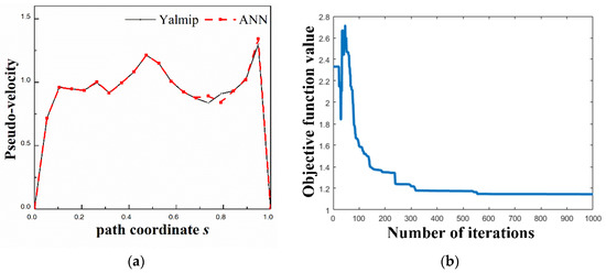
Figure 4.
Optimized results for robot joint solved by Yalmip with the method in reference and the proposed method using ANN. (a) Optimization variable h(sj) values at different coordinates; (b) Convergence curve of optimization objective with ANN.
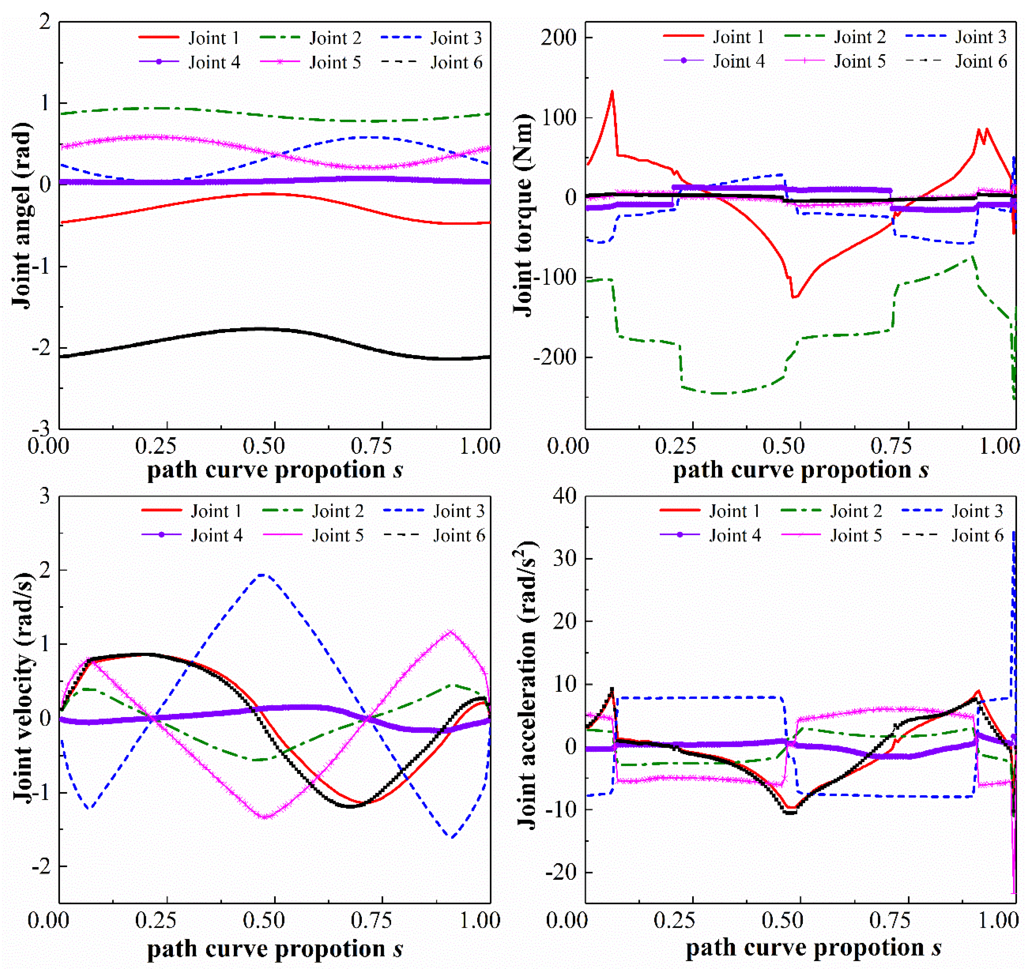
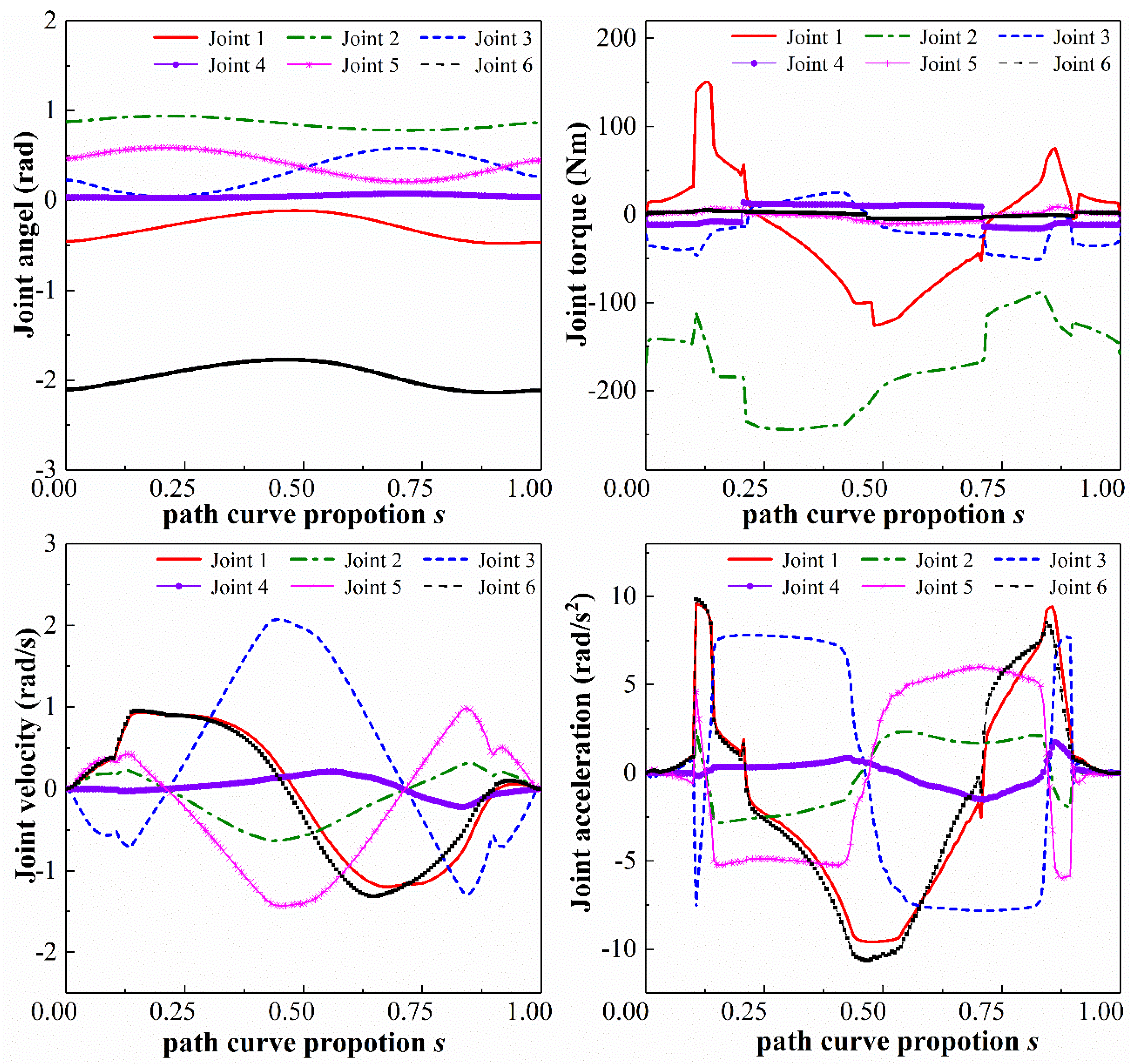
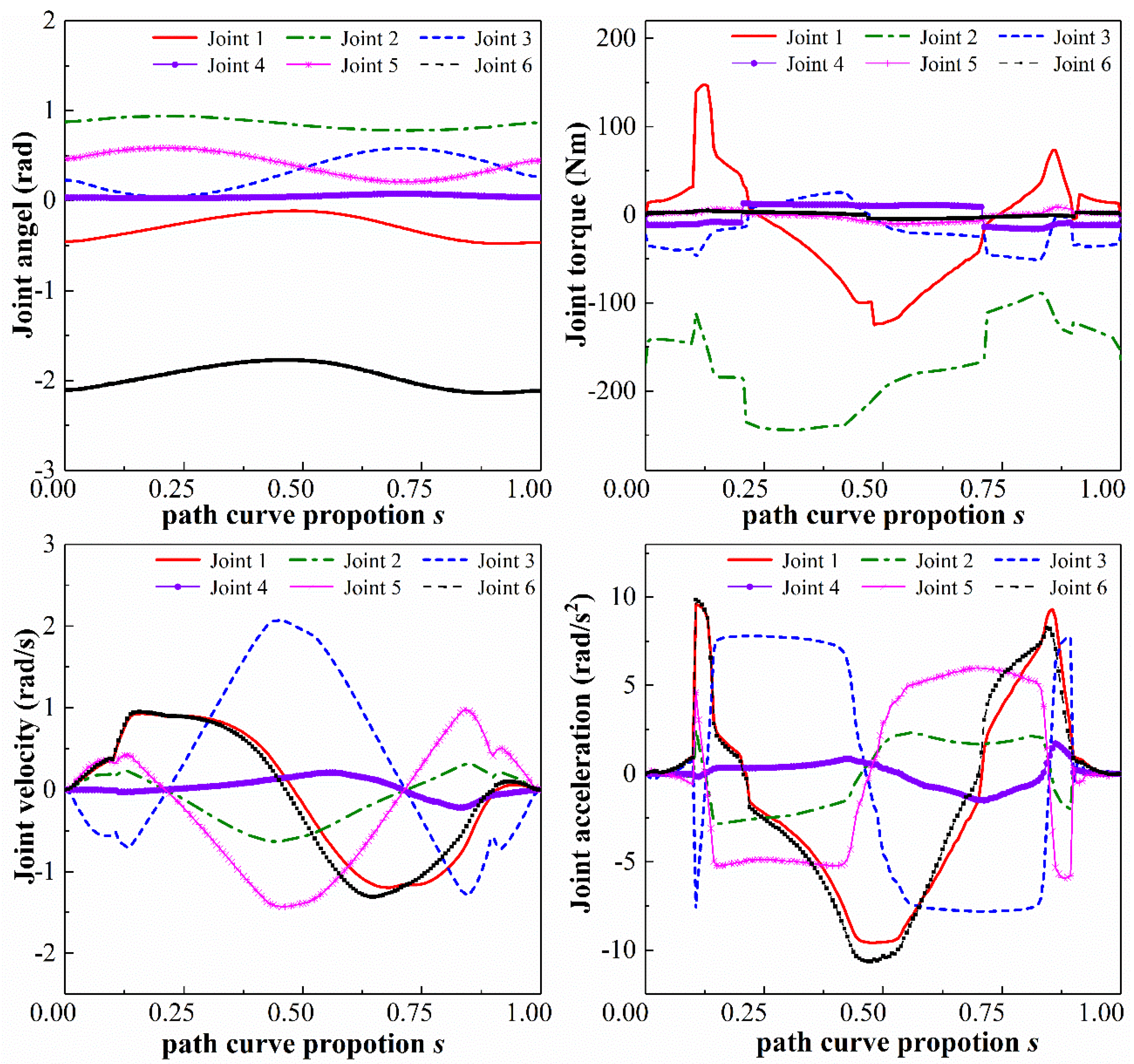
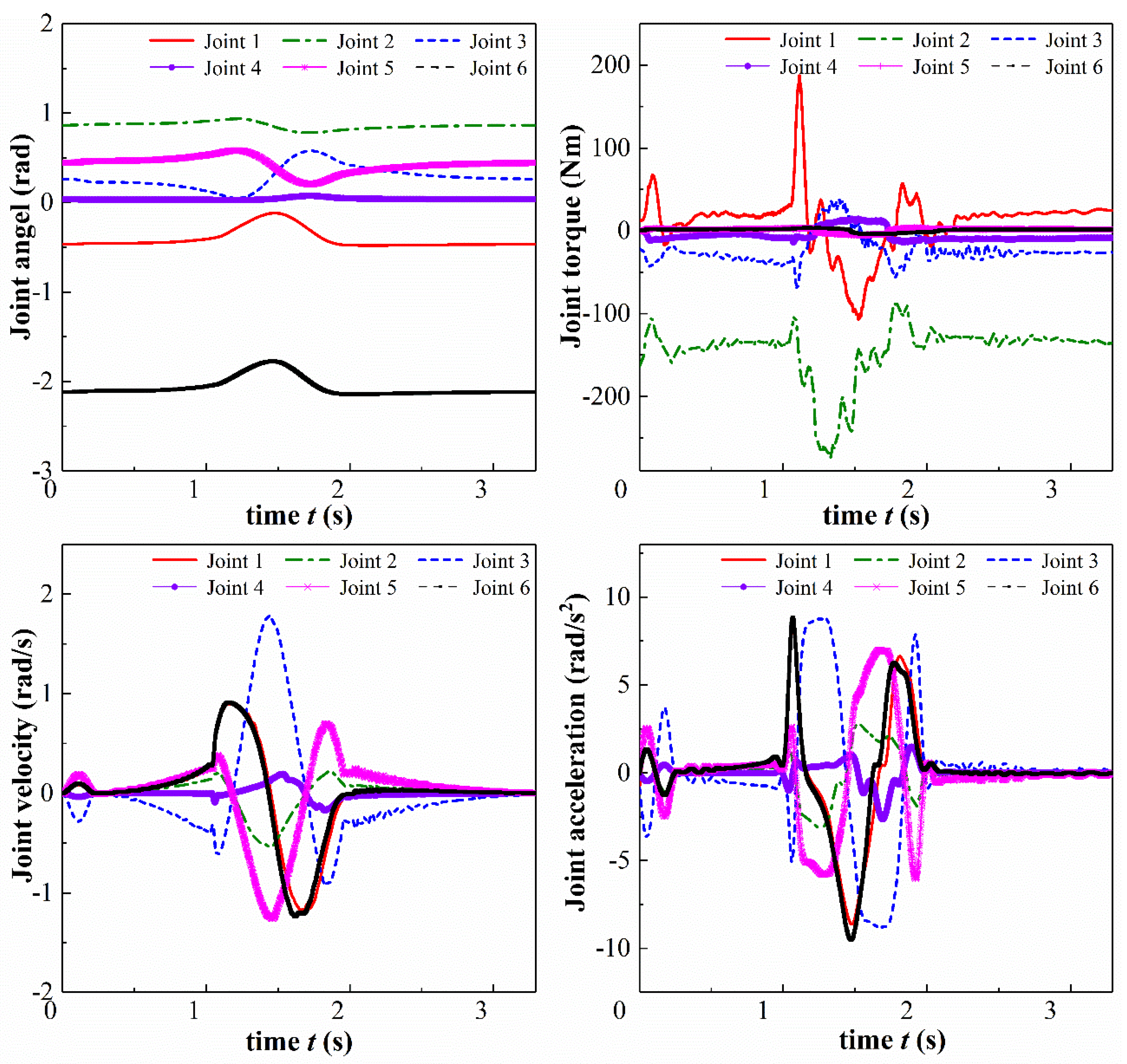
To intuitively display the motion of the robot, the joint angles and joint angular velocities and torques of six joints during the trajectory operation with time-energy optimization weight are obtained according to the method in [3] and our proposed method with bounded velocity, acceleration, torque limits, and initial and final boundaries, as shown in Figure 5 and Figure 6.
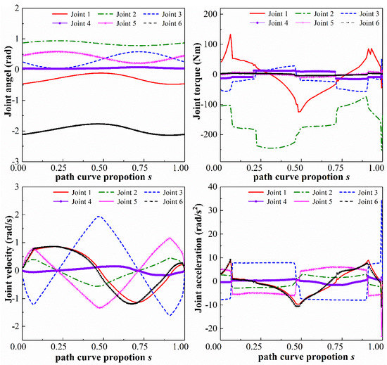
Figure 5.
Optimized trajectories for robot joint with the method in reference.
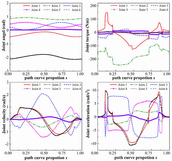
Figure 6.
Optimized trajectories for robot joint with the proposed method.
The joint angular velocity and acceleration curves start with non-zero values calculated by the method in [3], and accelerations of joints 2, 3 and 5 exceed the limits by 3.277 rad/s2, 26.674 rad/s2, 7.620 rad/s2, respectively. The generated trajectories are hardly used in the actual scene. On the contrary, our result showed a smoother optimization trajectory with initial and final zero velocity and acceleration and all kinematic and dynamic constraints were satisfied within the extreme values.
For verification of the effectiveness of the proposed method, the calculated normalized energy consumption and motion time tf results obtained by the proposed optimization model are listed in Table 3, when weights β = 0, 0.1, 1 and 100.4, of which selected weights β are the same as [3]. In Table 3, the motion time tf rises and the normalized energy decreases simultaneously when the weight increases, which indicates that the proposed trajectory optimization model can adjust the variable values according to the requirement of high-speed motion or low energy consumption.
Table 3.
Normalized energy consumption and motion time results obtained by the proposed optimization model.
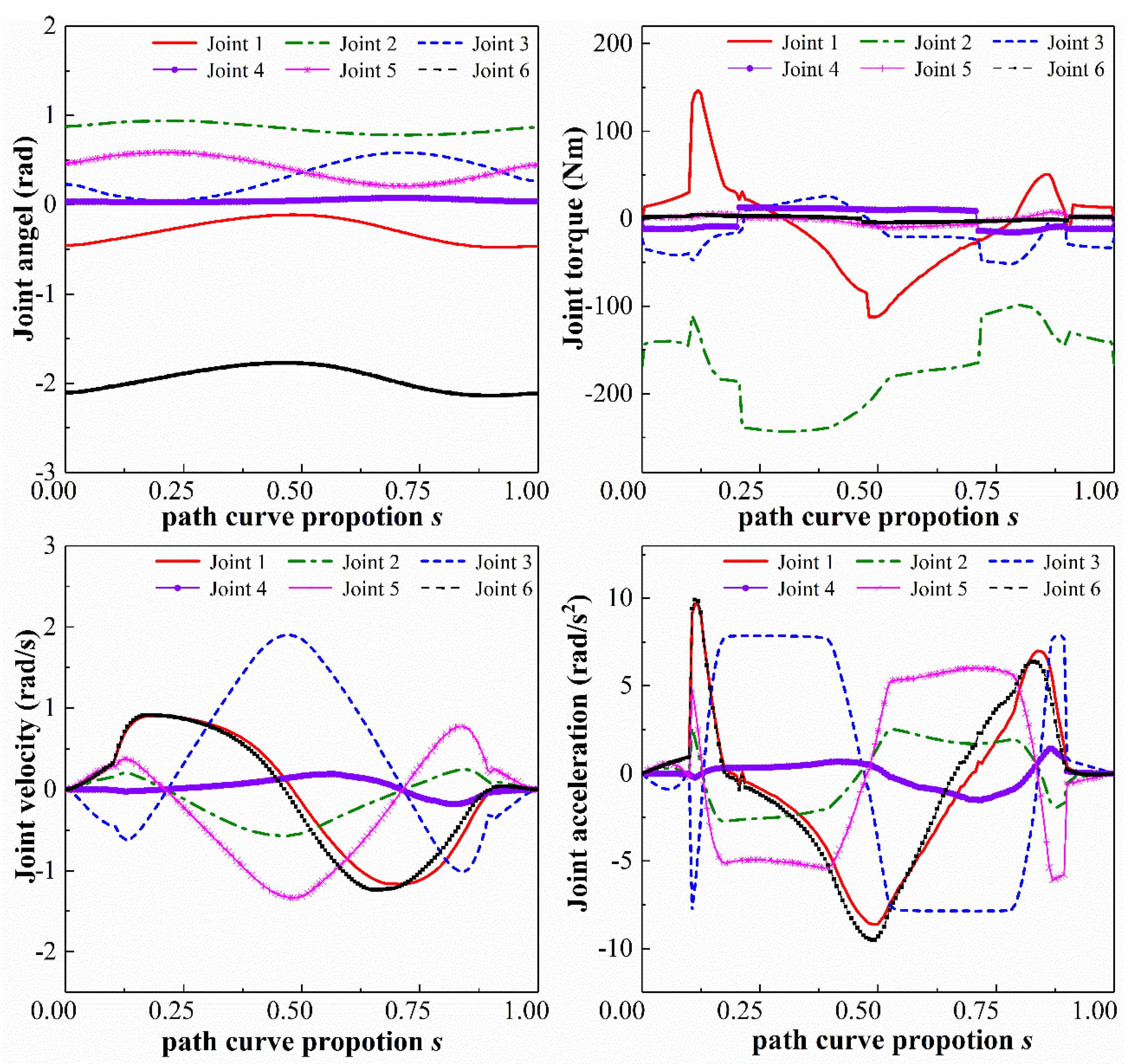
The results of the optimization trajectories with different weights β = 0.1 and 1 can be seen in Figure 7 and Figure 8. As can be seen in Figure 6, Figure 7 and Figure 8, the trajectory acceleration fluctuation at the corresponding singular point decreases gradually with weight increases. This indicates that the design of the objective function is based on the trade-off analysis of time and energy consumption. Therefore, the overall trend of the joint torque curve of the manipulator still tends to be near the safety limit of the rated torque. However, after the energy consumption modeling and weight distribution of the manipulator servo drive control system, the operation trend of the manipulator joint torque curve tends to decrease with increase in the weight. The time near the safety limit of the rated torque gradually decreases, which also means that the energy consumption of the joint servo drive control system has been effectively improved during the corresponding trajectory operation. From the normalized comparison of energy consumption in Table 3 of the manipulator trajectory optimization, it can be seen that modeling the energy consumption index of the robot servo motor and assigning a corresponding weight design plays a significant role in reducing the energy consumption value of the manipulator trajectory operation.
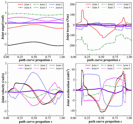
Figure 7.
Optimized trajectories for robot joint with the proposed method when α = 0.1.
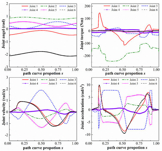
Figure 8.
Optimized trajectories for robot joint with the proposed method when α = 1.
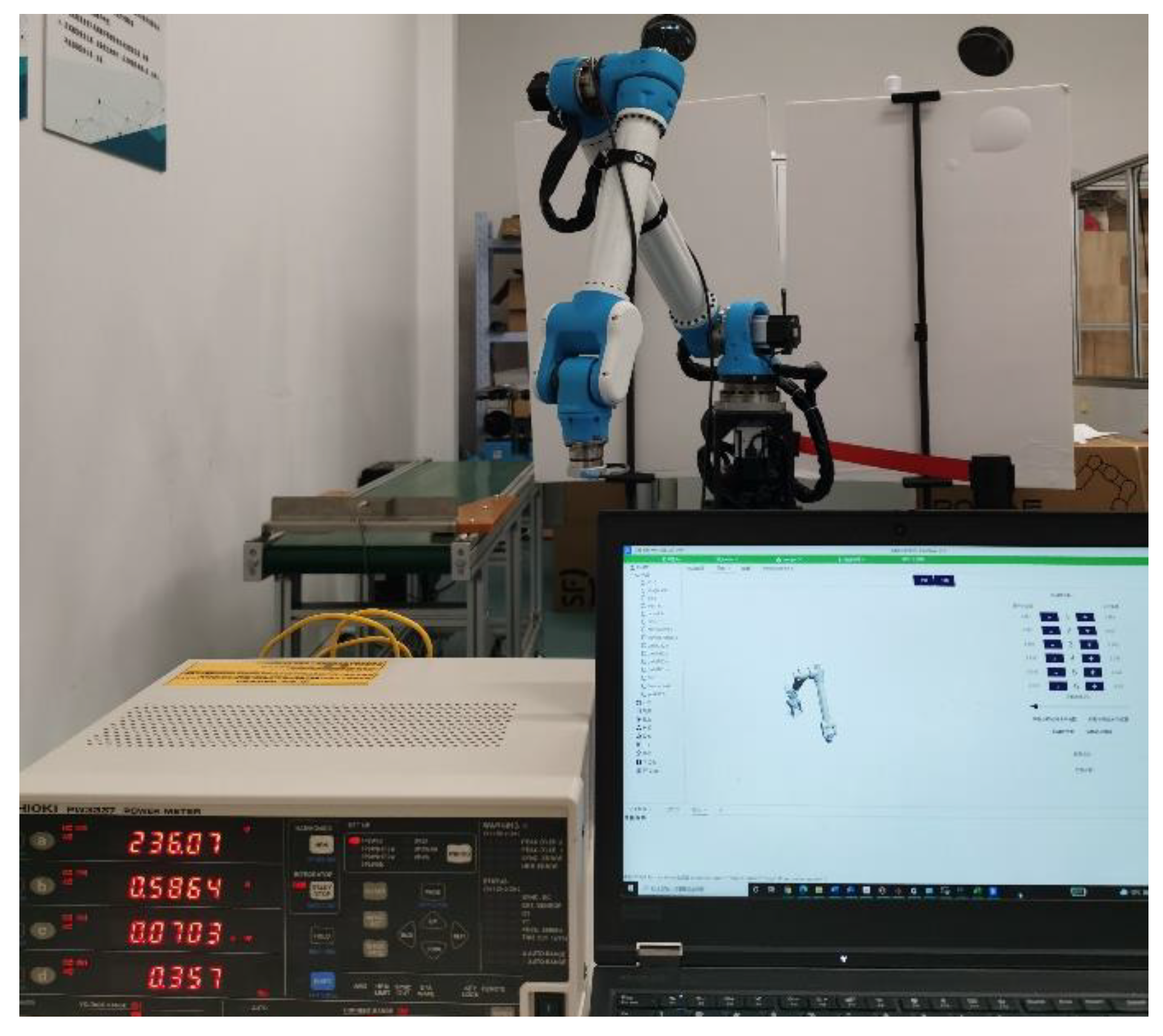
To test the actual optimization effect, an experiment of the proposed method was implemented with the robot system, as shown in Figure 9. The path time of the optimal trajectory when was 3.2915 s which ensured the joint velocity in the range of the velocity set limits. The energy consumption of the robot running optimal trajectory was 0.357 Wh. The experimental sampling data of six joint angles, torques and velocities of time-energy consumption optimal trajectory are shown in Figure 10. The torque values of the servo motor of joints were within the torque performance constraints. The safety range of the accelerations of robot joint was reached at several discrete solutions, and the obtained solutions were used in an actual scene, which demonstrated the effectiveness of the above algorithm and the constraint design.

Figure 9.
Experiment platform of six-joints robot.
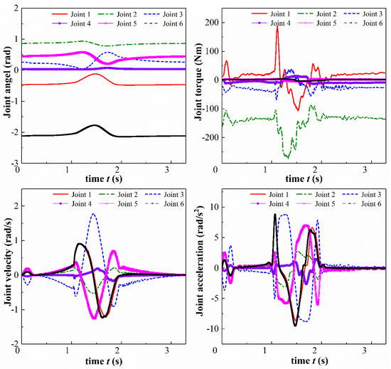
Figure 10.
Experiment data of optimal trajectory with α = 100.4.
7. Conclusions
To describe the optimization problem of robot trajectory planning, a time-energy optimization model based on the ANN algorithm was proposed in this paper. The energy consumption model of servo resistance loss was constructed in addition to motion time. For a six degrees of freedom industrial robot, the kinematics and dynamics impact on the coupling constraint condition were considered, including velocity, acceleration and torque. The optimization model was discretized based on the Riemann approximation method. Based on the established kinematic and dynamic model of the robot, a basic discretization model in terms of the generalized path variable mapping was constructed. Forward-substitution interpolation functions were presented as basic functions for the insurance of the initial and final zero-velocity and zero-acceleration of indirect kinematic expressions introduced in the discrete optimization model. Finally, the trajectory optimization parameters and the comprehensive tradeoff time-resistance energy loss index with multi-level performance constraints were solved by a numerical iterative solution strategy based on neural networks. The simulation and actual experiments were implemented with different optimization weights. The proposed method could enhance the acceleration control performance of the solved robot trajectory by reducing accelerations exceeding values of joint 2, 3 and 5 by 3.277 rad/s2, 26.674 rad/s2, 7.620 rad/s2, respectively. Moreover, comparison results between our method and recent optimization methods showed that the improved basic function contributes to the smoothness of the optimization trajectory and guarantees zero velocity and acceleration at the starting and ending points.
Author Contributions
Conceptualization, J.N.; methodology, R.H.; software, B.H., X.Y. and Q.M.; validation, T.R.; formal analysis, Y.G.; writing—original draft preparation, R.H.; writing—review and editing, T.R.; funding acquisition, J.N. All authors have read and agreed to the published version of the manuscript.
Funding
This research was funded by the Key Research and Development Program of Zhejiang province, No. 2020C01026.
Institutional Review Board Statement
Not applicable.
Informed Consent Statement
Not applicable.
Data Availability Statement
Not applicable.
Conflicts of Interest
The authors declare no conflict of interest.
Nomenclature
| αi−1 | Link twist | Joint torques derived by the iterative Newton–Euler formulation | |
| ai−1 | Link length | Inertia moment for rotor and gears of actuator i | |
| di | Link offset | , | Viscous and Coulomb friction coefficients |
| θi | Joint angle | Inertia tensor related to center of mass | |
| Link mass | Inertia tensor related to the origin of joint coordinate | ||
| Joint torque | , , , , , | Inertia moment components of link i | |
| Friction torque | Regressor matrix | ||
| Inertia torque | Subset of the independent columns of | ||
| q | Joint position vector | Coordinates of center of mass | |
| Velocity | Standard parameters for joint i | ||
| Acceleration | Minimal set vector of identifiable parameters | ||
| Torques vector | Mass or inertia matrix | ||
| t | Time | Coriolis and centrifugal vector | |
| Total motion time | Resistance energy consumption of the servo circuit in robot joint | ||
| Gravity | Weight coefficient of energy consumption | ||
| Electric current | s | Trip proportion assigned to path curve | |
| Resistance | The j-th point proportion of the divided path curve | ||
| Polynomial coefficients | Second order derivative of s | ||
| Observation matrix | First order derivative of s | ||
| N | Point number | Cubic Bezier curve function | |
| rx,ry,rz | Pose orientation vector | l | Half of the added continuous selected points number |
| v(sj) | Discrete optimization objective | d | The nearest integer less than or equal to 0.1(N−1) |
| Cost functions | H | Population of pattern solution | |
| Iteration index | Population of weight | ||
| TF | Transfer function | Random number |
Appendix A
The minimum identification parameter set is shown in Table A1.
Table A1.
Elements of the calculated minimum identification set .
Table A1.
Elements of the calculated minimum identification set .
| (1) | (2) | (3) | (4) | (5) | (6) | (7) |
| 14.2652 | 7.7347 | 13.4288 | 19.2053 | 0.3683 | −13.2957 | 20.0815 |
| (8) | (9) | (10) | (11) | (12) | (13) | (14) |
| −0.6178 | 0.0673 | 1.0250 | 33.5249 | 26.4618 | −0.0689 | 4.9279 |
| (15) | (16) | (17) | (18) | (19) | (20) | (21) |
| 4.0606 | 4.6718 | 0.3442 | 1.4541 | −0.8636 | −0.4512 | 10.7137 |
| (22) | (23) | (24) | (25) | (26) | (27) | (28) |
| 12.0429 | 0.0897 | 0.0388 | −0.0721 | 0.1035 | −0.0151 | 0.7826 |
| (29) | (30) | (31) | (32) | (33) | (34) | (35) |
| −0.4236 | −0.2792 | 8.4568 | 11.0075 | 0.0457 | 0.1336 | −0.0042 |
| (36) | (37) | (38) | (39) | (40) | (41) | (42) |
| 0.3912 | 0.0167 | 0.1285 | −0.3073 | −0.6151 | 1.4333 | 1.9285 |
| (43) | (44) | (45) | (46) | (47) | (48) | (49) |
| −0.0537 | −0.0283 | 0.0152 | −0.1652 | 0.0156 | −0.0056 | 0.0453 |
| (50) | (51) | (52) | ||||
| 0.1991 | 1.009 | 2.0133 |
References
- Verscheure, D.; Demeulenaere, B.; Swevers, J.; De Schutter, J.; Diehl, M. Time-Energy Optimal Path Tracking for Robots: A Numerically Efficient Optimization Approach. In Proceedings of the 2008 10th IEEE International Workshop on Advanced Motion Control, Trento, Italy, 26–28 March 2008; pp. 727–732. [Google Scholar]
- Riazi, S.; Wigström, O.; Bengtsson, K.; Lennartson, B. Energy and Peak Power Optimization of Time-Bounded Robot Trajectories. IEEE Trans. Autom. Sci. Eng. 2017, 14, 646–657. [Google Scholar] [CrossRef]
- Verscheure, D.; Demeulenaere, B.; Swevers, J.; De Schutter, J.; Diehl, M. Time-Optimal Path Tracking for Robots: A Convex Optimization Approach. IEEE Trans. Autom. Control. 2009, 54, 2318–2327. [Google Scholar] [CrossRef]
- Steinhauser, A.; Swevers, J. An Efficient Iterative Learning Approach to Time-Optimal Path Tracking for Industrial Robots. IEEE Trans. Ind. Inform. 2018, 14, 5200–5207. [Google Scholar] [CrossRef]
- Chen, D.; Li, S.; Li, W.; Wu, Q. A Multi-Level Simultaneous Minimization Scheme Applied to Jerk-Bounded Redundant Robot Manipulators. IEEE Trans. Autom. Sci. Eng. 2020, 17, 463–474. [Google Scholar] [CrossRef]
- Zhang, Y.; Li, S.; Gui, J.; Luo, X. Velocity-Level Control With Compliance to Acceleration-Level Constraints: A Novel Scheme for Manipulator Redundancy Resolution. IEEE Trans. Ind. Inform. 2018, 14, 921–930. [Google Scholar] [CrossRef]
- Nagy, Á.; Vajk, I. Sequential Time-Optimal Path-Tracking Algorithm for Robots. IEEE Trans. Robot. 2019, 35, 1253–1259. [Google Scholar] [CrossRef]
- Yuille, A.L.; Rangarajan, A. The Concave-Convex Procedure. Neural Comput. 2003, 15, 915–936. [Google Scholar] [CrossRef] [PubMed]
- Verscheure, D.; Diehl, M.; De Schutter, J.; Swevers, J. On-Line Time-Optimal Path Tracking for Robots. In Proceedings of the 2009 IEEE International Conference on Robotics and Automation, Kobe, Japan, 12–17 May 2009; pp. 599–605. [Google Scholar]
- Feng, Y.; Ji, Z.; Gao, Y.; Zheng, H.; Tan, J. An Energy-Saving Optimization Method for Cyclic Pick-and-Place Tasks Based on Flexible Joint Configurations. Robot. Comput. -Integr. Manuf. 2021, 67, 102037. [Google Scholar] [CrossRef]
- Palleschi, A.; Garabini, M.; Caporale, D.; Pallottino, L. Time-Optimal Path Tracking for Jerk Controlled Robots. IEEE Robot. Autom. Lett. 2019, 4, 3932–3939. [Google Scholar] [CrossRef]
- Ramezani, N.; Williams, M.-A. Smooth Robot Motion with an Optimal Redundancy Resolution for PR2 Robot Based on an Analytic Inverse Kinematic Solution. In Proceedings of the 2015 IEEE-RAS 15th International Conference on Humanoid Robots (Humanoids), Seoul, Korea, 3–5 November 2015; pp. 338–345. [Google Scholar]
- He, T.; Zhang, Y.; Sun, F.; Shi, X. Immune Optimization Based Multi-Objective Six-DOF Trajectory Planning for Industrial Robot Manipulators. In Proceedings of the 2016 12th World Congress on Intelligent Control and Automation (WCICA), Guilin, China, 12–15 June 2016; pp. 2945–2950. [Google Scholar]
- Abu-Dakka, F.J.; Assad, I.F.; Alkhdour, R.M.; Abderahim, M. Statistical Evaluation of an Evolutionary Algorithm for Minimum Time Trajectory Planning Problem for Industrial Robots. Int. J. Adv. Manuf. Technol. 2017, 89, 389–406. [Google Scholar] [CrossRef]
- Tang, X.; Shi, C.; Deng, T.; Wu, Z.; Yang, L. Parallel random matrix particle swarm optimization scheduling algorithms with budget constraints on cloud computing systems. Appl. Soft Comput. 2021, 113, 107914. [Google Scholar] [CrossRef]
- Villarrubia, G.; De Paz, J.F.; Chamoso, P.; la Prieta, F.D. Artificial Neural Networks Used in Optimization Problems. Neurocomputing 2018, 272, 10–16. [Google Scholar] [CrossRef]
- Sadollah, A.; Sayyaadi, H.; Yadav, A. A Dynamic Metaheuristic Optimization Model Inspired by Biological Nervous Systems: Neural Network Algorithm. Appl. Soft Comput. 2018, 71, 747–782. [Google Scholar] [CrossRef]
- Shi, X.; Fang, H.; Pi, G.; Xu, X.; Chen, H. Time-Energy-Jerk Dynamic Optimal Trajectory Planning for Manipulators Based on Quintic NURBS. In Proceedings of the 2018 3rd International Conference on Robotics and Automation Engineering (ICRAE), Guangzhou, China, 17–19 November 2018; pp. 44–49. [Google Scholar]
- Craig, J. Introduction to Robotics: Mechanics and Control, 3rd ed.; Pearson Education: Hoboken, NJ, USA, 2005. [Google Scholar]
- Khalil, W.; Gautier, M.; Lemoine, P. Identification of the Payload Inertial Parameters of Industrial Manipulators. In Proceedings of the 2007 IEEE International Conference on Robotics and Automation, Rome, Italy, 10–14 April 2007; pp. 4943–4948. [Google Scholar]
- Jin, J.; Gans, N. Parameter Identification for Industrial Robots with a Fast and Robust Trajectory Design Approach. Robot. Comput. Integr. Manuf. 2015, 31, 21–29. [Google Scholar] [CrossRef]
- Gautier, M. Numerical Calculation of the Base Inertial Parameters of Robots. J. Robot. Syst. 1991, 8, 485–506. [Google Scholar] [CrossRef]
- Dmitruk, A.V.; Kaganovich, A.M. The Hybrid Maximum Principle Is a Consequence of Pontryagin Maximum Principle. Syst. Control. Lett. 2008, 57, 964–970. [Google Scholar] [CrossRef] [Green Version]
- Sciavicco, L.; Siciliano, B. Dynamics. Modelling and Control of Robot Manipulators; Sciavicco, L., Siciliano, B., Eds.; Springer: London, UK, 2000; pp. 131–183. ISBN 978-1-4471-0449-0. [Google Scholar]
Publisher’s Note: MDPI stays neutral with regard to jurisdictional claims in published maps and institutional affiliations. |
© 2022 by the authors. Licensee MDPI, Basel, Switzerland. This article is an open access article distributed under the terms and conditions of the Creative Commons Attribution (CC BY) license (https://creativecommons.org/licenses/by/4.0/).