Article

Modeling and Control Design of a Contact-Based, Electrostatically Actuated Rotating Sphere

1
Chair of Control Engineering, University of Augsburg, 86159 Augsburg, Germany
2
Chair of Microsystems Technology, Ruhr-Universität Bochum, 44801 Bochum, Germany
*
Authors to whom correspondence should be addressed.
Actuators 2022, 11(3), 90; https://doi.org/10.3390/act11030090
Submission received: 31 January 2022 / Revised: 9 March 2022 / Accepted: 12 March 2022 / Published: 15 March 2022
(This article belongs to the Section Miniaturized and Micro Actuators)

Abstract

:
The performance of micromirrors in terms of their maximum deflection is often limited due to mechanical constraints in the design. To increase the range of achievable deflection angles, we present a novel concept in which a free-lying sphere with a flat side as reflector can be rotated. Due to the large forces needed to move the sphere, multiple electrostatic actuators are used to cooperatively rotate the sphere in iterative steps by impacts and friction. A parameterized system-level model of the configuration is derived, which considers arbitrary multi-contact scenarios and can be used for simulation, analysis, and control design purposes. Due to the complex, indirect relation between the actuator voltages and the sphere motion, model-based numerical optimization is applied to obtain suitable system inputs. This results in rotation sequences, which can be understood as a sequence of motion primitives, thus transforming the continuous time model into an abstract discrete time model. Based on this, we propose a feedback control strategy for trajectory following, considering model uncertainties by a learning scheme. High precision is achieved by an extension controlling the angular change of each rotation step. The suitability of the overall approach is demonstrated in simulation for maximum angles of 40°, achieving angular velocities of approximately 10°/s.

1. Introduction

Optical actuators find numerous applications in industry and consumer markets, especially in the field of laser scanners, which includes displays, projectors or barcode scanners [1]. Due to their small dimensions, micro-electro mechanical systems make a major contribution to this. Both resonant and non-resonant micromirror devices are used for these applications. Resonant actuators are often used for raster-scan applications [2] and non-resonant ones for vector-scan applications [3].
These actuations are performed electrostatically [4], electromagnetically [5] or piezoelectrically [6]. Especially for optical applications, large deflection angles are required in general. Comparing these actuation concepts, electromagnetic actuation is commonly used for applications that allow a large deflection angle quasi-statically and are operated non-resonantly [7]. Electrostatic micromirror devices are usually operated resonantly, as they only provide low forces and the angular deflection is limited by construction. Compared to electromagnetic concepts, small deflection angles can be achieved with digital mirror devices [8].
In order to circumvent the constructional limitations of a micromirror, Bunge et al. presented a concept in which a free-lying spherical cap, which is not connected to the actuator, is rotated electrostatically [9]. This avoids the aforementioned angle limitation, as there are no restoring forces due to mechanical connections. The stainless steel ball is rotated using a combination of parallel plate actuation and comb-drives. By superimposing these movements, a rotation of the ball is caused due to the stick-slip effect. When operated in resonance, a mechanical deflection of ±35.2° could be achieved. As part of the research project Kick and Catch [10], the concept proposed here is non-resonant and generates a fast and large impulse on the sphere via multiple lever actuators. By actively controlling the individual actuator movements, a kick and rotation phase can be initiated, in which the sphere is kicked upwards with a spin. A free flight phase avoids unwanted crosstalk, which means that the ball rotates freely. The flight phase is completed by a predefined landing (catch).
A challenge of this actuation principle lies in the control of the sphere rotation since there is no trivial relation between the voltages applied to the electrostatic actuators and the resulting sphere motion. This is mostly due to the fact that the sphere can only be influenced indirectly by impact and friction with the actuator tips. Moreover, there is no intuitive method how to choose the time course of the applied voltages for each actuator in an optimal way.
For a systematic approach, mathematical models for analysis and simulation are therefore useful. While different modeling approaches have been proposed in literature, the choice of the applied method often depends on the system to be modeled, as well as the desired level of detail. In the case of purely mechanical systems, models can be obtained based on vibration responses, which additionally allow fault detection [11]. For the simulation and analysis of systems within different physical domains, bond graph methods have shown to be useful [12]. However, an additional model based on differential equations has to be derived for the design of controller or observer architectures. In the field of microelectromechanical systems, these are commonly obtained by numerical methods such as finite element modeling [13]. While such models can achieve high accuracy, their suitability for extensive simulation and evaluation of control strategies may be limited due to large computation times. Mathematical model order reduction can be applied to reduce the model complexity, thus simplifying the control design [14]. In contrast, the direct derivation of system-level models such as in [15] often yields a sufficient quality for basic analysis and control design purposes. For the presented micromirror, this requires modeling strategies for contact and friction dynamics.
A straightforward method to model contacts consists of a permanent evaluation of contact conditions and subsequent application of the momentum conservation principle [16]. However, this assumes infinitesimal contact duration, which is not the case for lasting contacts and sliding motions assumed to affect the sphere motion. This limitation does not hold for the method of dimensionality reduction [17], in which a three-dimensional contact surface is transformed into a one-dimensional expression. The subsequent force computation is based on the Hertzian model [18], describing the contact surface as an array of damped springs. While this method can achieve highly accurate results and is exact for (visco-)elastic problems, its implementation is time-consuming and computationally expensive for complex multi-contact systems with varying contact surfaces. Since the presented actuator is assumed to behave rigidly, the contacts may be reduced to single points. We therefore apply the less accurate but significantly simpler approach of power-based restriction functions by Specker et al. [19], in which also a viscoelastic approximation is used. Its advantage lies in the low implementation effort and the direct integration within the Lagrange formalism.
The model can then be used for the controller design. In case of the presented micromirror, this includes two steps: First, suitable voltages for the electrostatic actuation have to be derived, leading to a successful rotation. Since the sphere stably remains in its new position, the resulting system can then be interpreted as a discrete system with a discrete set of inputs corresponding to different kick directions. In a second step, a discrete feedback control approach successively drives the sphere such that the desired, possibly time-varying, reference angles are followed. Suitable control concepts include model-predictive control [20], supervisory control [21] by prior reformulation into a finite state automaton, and approaches using machine learning such as state vector machines [22] and reinforcement learning [23]. In contrast to purely model-based concepts, machine learning has the advantage that systematic model errors can be compensated by either learning the optimal state-input relation or the model directly.
The main goal of this work is to derive a system-level model of a complex, contact-based micromirror for simulation, control design, and optimization purposes. This model is subsequently used to design a feedback controller. An extension is proposed to efficiently take into account model mismatch by adaptive direction parameters and neural networks, and its suitability is shown in simulation with a non-ideal, perturbed model. The proposed concept may be used as a digital micromirror with the advantage that any angular state can be adopted instead of a set of discrete positions.
This work is organized as follows: In Section 2, the actuator design is presented and a system-level model is derived in Section 3. Based on this model, an optimal actuation principle and a feedback control strategy are described in Section 4. The simulation results demonstrating the suitability of the approach are given in Section 5, followed by a discussion in Section 6 and concluding remarks in Section 7.

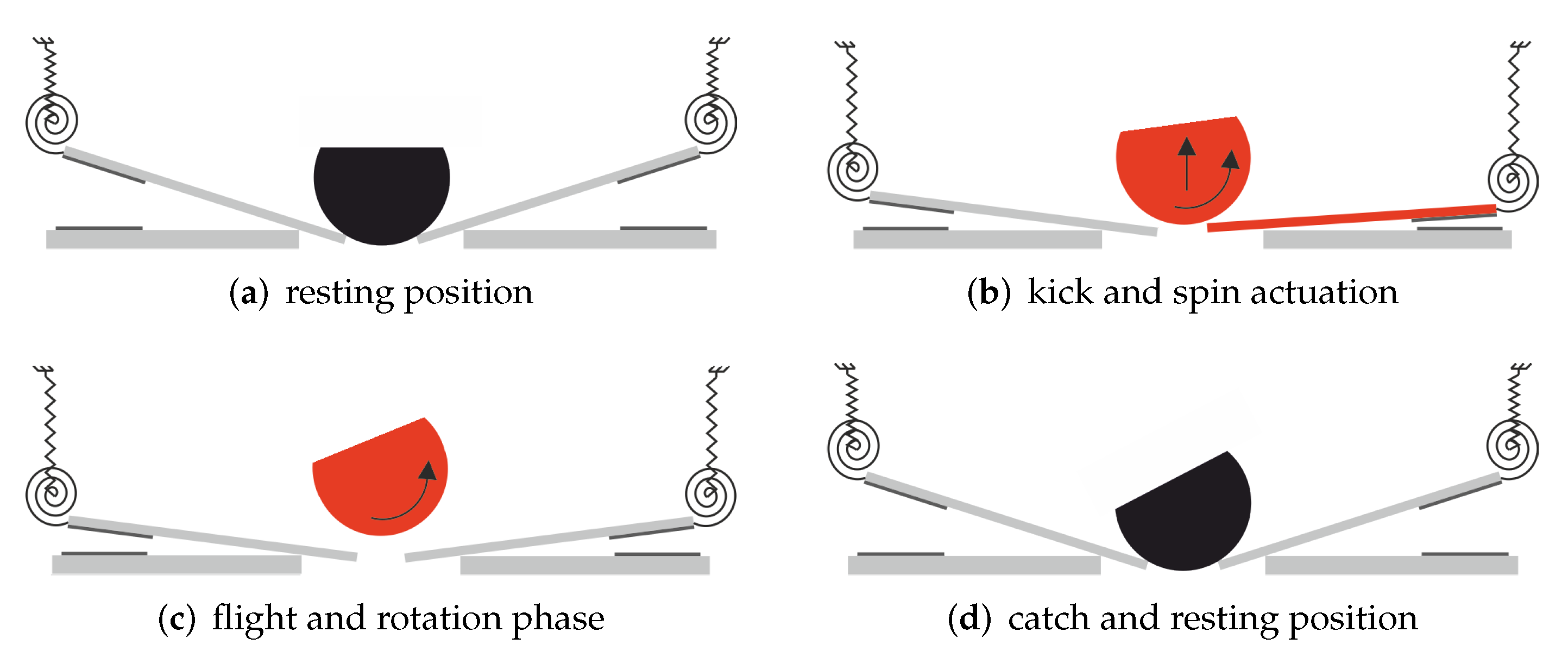
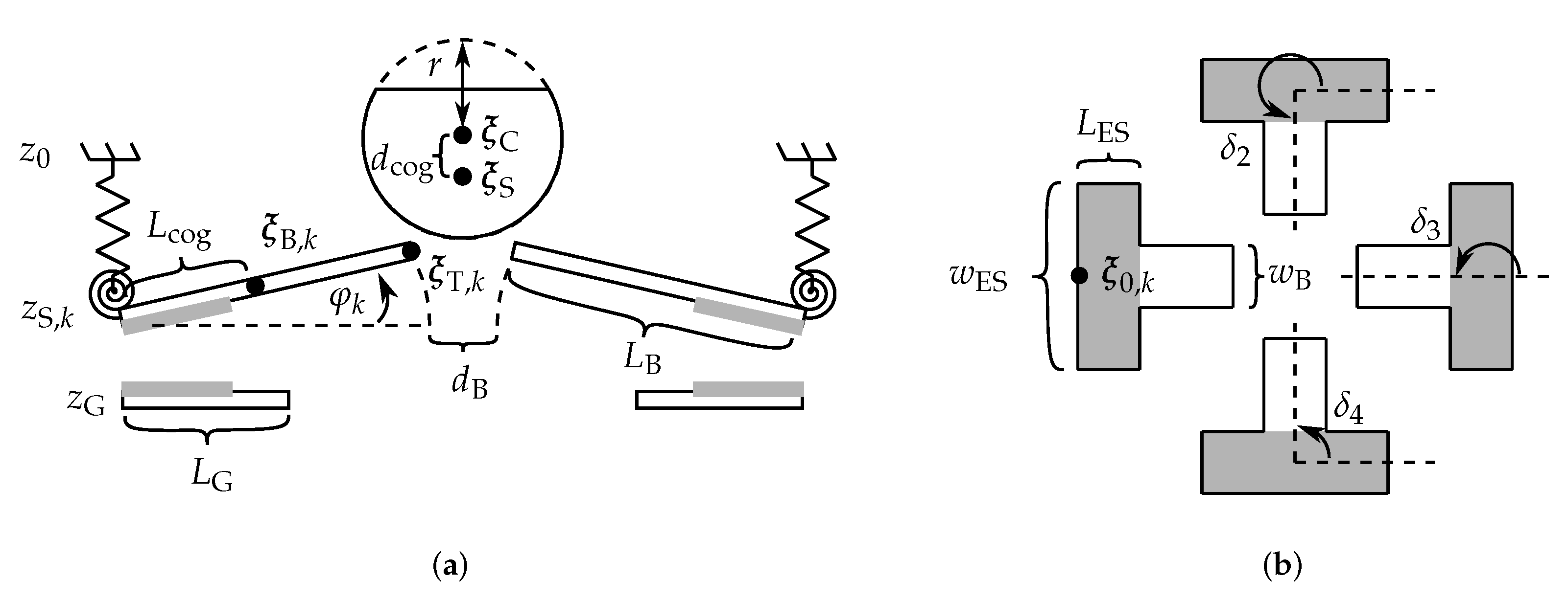
2. Actuator Design and Working Principle

The micromirror system consists of four symmetrically arranged, suspended beams, which sections close to the suspensions form parallel plate actuators with the ground plate. The sphere is initially placed on the beam tips in the center of the setup and has a diameter of 2 mm. The side view of the design is sketched in Figure 1 and illustrates the actuation phases. Here, each lever actuator is connected to the substrate via solid state springs. These allow a rotation of the lever, but also a linear and vertical deflection. This is intended to both, to provide stable bearing and to achieve the necessary actuation. The force required for the sphere to enter the kick and spin phase is generated by applying a voltage to the actuator, pulling the movable beam downwards. Here, we deliberately make use of the pull-in instability to achieve high beam velocities and large strokes. The energy generated in this way is then transferred to the sphere with a mechanical lever. The contact point between the beam and the ground plate thereby serves as center of rotation of the beam. By asymmetrically actuating the four beams, a rotation of the sphere in a free flight phase is achieved. In such a concept, the contact between the actuator and the sphere is of particular importance, requiring precise analysis and modeling.

3. Modeling

The sphere rotation can only be adjusted indirectly, i.e., by impacts and friction between the electrostatically actuated beams and the sphere. For such complex systems, data-based control approaches can be of advantage and the data may be obtained by real measurements. However, the data generation process can be automated and largely simplified by simulation of a system model.
For the purpose of obtaining the rotational motion of the sphere, we first derive the general equations of motion of the individual partial systems, i.e., the electrostatic actuators and the sphere, by a Lagragian approach and then extend the dynamics by their coupling in terms of contact and friction. We can describe each partial system by a vector of generalized coordinates q , which correspond to the translatory and rotatory degrees of freedom. The equations of motion are then obtained by
d d t T q ˙ T q + V q = Q ,
with the kinetic and potential energies T ( q , q ˙ ) , V ( q ) and the nonconservative or external generalized forces Q .

3.1. Electrostatic Actuator Dynamics

The overall system consists of four electrostatic actuators with a movable beam, and the respective electrode area has the dimension L ES × w ES . Here, the subscript ( · ) ES denotes the electrostatic partial system. In order to simplify the model, we assume the beams to be rigid and that their suspensions allow only vertical and torsional movements. We therefore approximate each suspension by a vertical and rotational spring. The parameters necessary for the following derivation are depicted in Figure 2. Note that the sketch is not to scale and its true dimensions are given in Table A1.
By using the generalized coordinates q B , k = [ z S , k , φ k ] of the k-th beam, the coordinate vector ξ B , k of its center of gravity corresponds to
ξ B , k = x B , k y B , k z B , k = L cog cos δ k cos φ k sin δ k cos φ k sin φ k + 0 0 z S , k z 0 + ξ 0 , k
with the suspension point
ξ 0 , k = ( L B + 0.5 d B ) cos δ k sin δ k 0 + 0 0 z 0 .
Given the gravitational constant g, mass m B , inertia J B , translatory and torsional stiffnesses k z and k φ , the respective energies can then be computed by
T B , k = 0.5 m B ξ B , k ξ B , k + 0.5 J B φ ˙ k 2 ,
V B , k = m B g z B , k + 0.5 k z ( z 0 z S , k ) 2 + 0.5 k φ φ k 2 .
Note that although the torsional and translatory spring stiffnesses may be nonlinear and will depend on both z and φ , we here assume an approximately linear, decoupled relation due to the small range of motion. The beam motion also depends on external forces Q B , k resulting from electrostatic actuation by applying a voltage V k ( Q ES , k ), the sphere contact at its tip ( Q BS , k ), and the impact with the ground plate ( Q BG , k ). The latter two will be derived later in Section 3.3. The electrostatic force is divided into a force F ES , k acting in negative vertical direction, and the electrostatic torque M ES , k influencing the beam rotation. These can be computed by the partial derivatives of the time-varying capacitance C k over the generalized coordinates, i.e.,
F ES , k = 0.5 V k 2 C k z S , k ,
M ES , k = 0.5 V k 2 C k φ k ,
resulting in Q ES , k = [ F ES , k , M ES , k ] . Here, we use the approximation
C k = ε 0 w ES θ k ln R k L k + 2 ε 0 w ES ln 2 π θ k 2 π θ k + ln 2 π 2 π θ k θ k
as given in [24,25] with
R k = L ES 2 + 2 z S , k + L ES sin ( φ k ) 2 sin ( | φ k | )
L k = R k L ES
θ k = | φ k | .
Note that we further assumed that the effect of the 300 nm thick insulation layer can be neglected in comparison with the 10 μm gap between the electrodes. Equation (8) and its partial derivatives are numerically problematic when being evaluated at angles θ k close to zero. For simulation purposes, we therefore approximate the capacitance by a black-box model. Here, we use a two-dimensional radial basis function network
C k = i n z j n φ a i , j exp ( z k c z , i ) 2 σ z 2 ( φ k c φ , j ) 2 σ φ 2
consisting of the sum of n z × n φ Gaussian functions with centers c z , i , c φ , j and variance σ z , σ φ , weighted by coefficients a i , j . For this approximation, we used 25 × 25 equidistantly distributed Gaussian functions with c z , i [ 9.9 , 3.3 ] μ m , c φ , j [ 14.5 , 4.5 ] × 10 3 , σ z = 0.5 μ m , and σ φ = 0.75 × 10 3 . The weighting parameters a i , j were obtained by a least squares approach. Finally, we take into account linear damping of the beam by forces
D B , k = d B , z z S , k d B , φ φ k
with positive coefficients d B , z , d B , φ . In summary, the beam dynamics are described by
M B , k q ¨ = m B g + 0.5 m B L cog sin φ k φ ˙ k 2 0.5 m B g L cog cos φ k K q + D B , k + Q ES , k + Q BS , k + Q BG , k
with mass and stiffness matrices
M B , k = m B 0.5 m B L cog cos φ k 0.5 m B L cog cos φ k J B + 0.25 m B L cog 2 , K = k z 0 0 k φ .

3.2. Sphere Dynamics

In contrast to the beams, which movements only take place within a single plane, the sphere motion has to consider all six degrees of freedom. As before, we define a vector of generalized coordinates q S = [ ξ S , ψ ] , describing the sphere position and rotation. Here, we use the coordinates ξ S = [ x S , y S , z S ] of the center of gravity of the spherical cap and the Cardan angles ψ = [ α , β , γ ] .
For the purpose of simplifying some parts of the derivation, we will use both the inertial and body frame coordinates. This means that we can describe an arbitrary vector r either in inertial frame coordinates, denoted by the left subscript I, i.e., I r , or in the coordinates of the rotated sphere frame, denoted by the subscript S as in S r . The vectors can be transformed using the rotation matrix S A I ( ψ ) from the inertial into the body frame, and back-transformed with its inverse I A S ( ψ ) = S A I ( ψ ) . Note that the same holds for the rotation velocity vector ω , and a missing left subscript also corresponds to the inertial frame. Moreover, it is important to mention that the Cardan angles ψ imply a subsequent rotation of the single angles in an invariant order. Thus, its derivative ψ ˙ is not identical to I ω or S ω , which corresponds to the current angular velocity in direction of the rotation axis. However, there is a transformation matrix ω T ψ ˙ ( ψ ) = ψ ˙ T ω 1 ( ψ ) for the respective conversion
S ω = ω T ψ ˙ ψ ˙
and its inverse. The transformation matrices are given in the Appendix A.1. For a deeper understanding, the interested reader is referred to [26].
We make use of the fact that the energy is independent of the coordinate system, in which it is evaluated. Thus, we can define the translatory and kinetic energies in the inertial and body frame, respectively. This results in
T S = 0.5 m S I ξ S I ξ S + 0.5 S ω S J S S ω ,
V S = m S g z S
with sphere mass m S . Note that due to the body frame formulation, we have a constant, diagonal inertia matrix S J S with respect to the center of gravity. Its detailed derivation is given in Appendix A.2. It is then possible to compute the rotational motion within the body frame, i.e.,
S J S S ω ˙ = S D ω + S q ω
and use the transformation (16) to obtain the Cardan angle derivative
ψ ¨ = ψ ˙ T ˙ ω S ω + ψ ˙ T ω S ω ˙ .
The translatory motion is given by
m S ξ ˙ S = D ξ + q ξ [ 0 , 0 , m S g ] .
In the above Equations (19) and (21), S Q ω , Q ξ are the external forces resulting from the sphere-beam contact and S D ω , D ξ correspond to the linear damping terms
S D ω = d ω S ω , D ξ = d ξ ξ ˙ S .

3.3. Contact and Friction Modeling

It remains to derive the coupling between the beams and the sphere in terms of friction and contact forces Q BS , k , S Q ω and Q ξ , as well as the impact forces Q BG , k between the movable beams and their respective ground plate. In the following, we will first explain the general approach based on [19] for the straightforward beam-ground impact, and then utilize the same concept for the beam-sphere contact including friction. One of the main advantages of the method lies in the direct implementation within the Lagrange formalism.

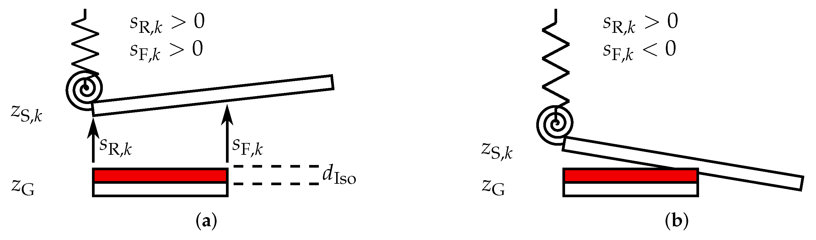
3.3.1. Beam-Ground Contact

When a high voltage is applied to one of the electrostatic actuators, the beam is attracted to the ground plate. Since the beam is longer than the ground plate, its tip then moves upwards with high velocity due to the leverage effect, until its suspended rear end impacts the ground plate. This suggests that the resulting contact forces are key elements of the working principle and have to be contained within the model. For this purpose, two contact points, namely at the rear and front end of the ground plate are investigated.
Instead of rigid contacts, which are problematic for numerical simulations due to discontinuities within the dynamics, we use a viscoelastic approximation similar to [19]. To this end, a small overlap s of the beam and the ground plate is allowed but results in a counteracting force, while energy loss during the contact is considered in dependence of the impact velocity v = s ˙ . Additional subscripts ( · ) R and ( · ) F denote the rear and front end contacts, and will be replaced by ( · ) * when valid for both cases. The overlap can be defined as the signed distance between the respective beam point and the ground plate as shown in Figure 3. It is important to mention that due to the numerical approximation using the overlap, a short circuit can occur within the simulation when the beam is in contact. In order to prevent this, an additional space denoted as virtual insulation layer, which is significantly thicker than the actual insulation layer, is inserted for numerical stabilization.
This results in
s R , k = z S , k ( z G + d Iso ) ,
s F , k = z S , k ( z G + d Iso ) + L G tan φ k .
The counteracting force F * , k is then obtained using an activation function R a , * ( s ) and a power function R p , * ( v ) by
F * , k = R a , * R p , * v * , k .
Here, we use a slight adaptation of the definition in [19]. According to [27] the activation function is then given by
R a , * = 0 , if s * , k 0 k c 2 4 C s * , k 2 , if 2 C k c < s * , k < 0 k c s * , k C , otherwise ,
which can be interpreted as the force characteristic of a nonlinear spring that is zero when no contact occurs ( s * , k 0 ), increases quadratically for s * , k < 0 until R a , * reaches the transition parameter C, and then has a linear stiffness k c . The energy loss during the impact is adjusted by the power function
R p , * = v * , k 2 log cosh ( r d v * , k ) 2 r d
with damping parameter r d . Each contact results in a generalized force Q * , k which takes into account the beam’s direction of action by a subsequent partial derivative with respect to q ˙ B , k , i.e.,
Q * , k = R a , * R p , * q ˙ B , k = F * , k v * , k q ˙ B , k ,
which is finally summarized into
Q BG , k = Q R , k + Q F , k .
Note that we here assumed negligibly low friction forces at the contact points due to mainly vertical impacts between the beam and the ground plate.

3.3.2. Beam-Sphere Contact

The same procedure can now be used for the beam-sphere contact by modifying the overlap s S , k of the k-th beam with the sphere. Here, we choose the penetration depth of the beam tip into the sphere surface. For this purpose, we define the center ξ C of the full sphere and the beam tip ξ T , k , which can be described as
ξ C = ξ S + r SC = ξ S + I A S [ 0 , 0 , d cog ]
and
ξ T , k = x T , k y T , k z T , k = L B cos δ k cos φ k sin δ k cos φ k sin φ k + 0 0 z S , k z 0 + ξ 0 , k .
Note that for the sphere center we made use of the fact that the vector r SC from the center of gravity to the full sphere center corresponds to a displacement d cog in z-direction of the body frame and can be back-transformed using the rotation matrix I A S . Given the sphere radius r it follows that
s S , k = ( ξ T , k ξ C ) ( ξ T , k ξ C ) r ,
and for its timed derivative
v S , k = 1 s S , k + r ( ξ T , k ξ C ) ( ξ ˙ T , k ξ ˙ C ) .
The overlap (32) allows us to compute the contact force F BS , k using (25)–(27), and for the calculation of Q BS , k by (28), it remains to determine the partial derivative of (33) over q ˙ B , k . For the nonconservative sphere forces Q ξ , S q ω , it is of advantage to derivate the overlap velocity over [ ξ ˙ S , S ω ] instead of q ˙ S = [ ξ ˙ S , ψ ˙ ] due to their direct dependence within the dynamics (19) and (21). To this end, we can write ξ ˙ C as
ξ ˙ C = ξ ˙ S + I ω × r SC = ξ ˙ S + I A S ( S ω × S r SC ) = ξ ˙ S d cog I A S 0 1 0 1 0 0 0 0 0 S ω
from which follows that
v S , k ξ ˙ S = v S , k ξ ˙ C
v S , k S ω = v S , k ξ ˙ C d cog I A S 0 1 0 1 0 0 0 0 0 .
The overall force moving the sphere corresponds to the sum of the single generalized forces induced by each beam, i.e.,
[ Q ξ , S Q ω ] = k F BS , k v S , k ξ ˙ S v S , k S ω .

3.3.3. Beam-Sphere Friction
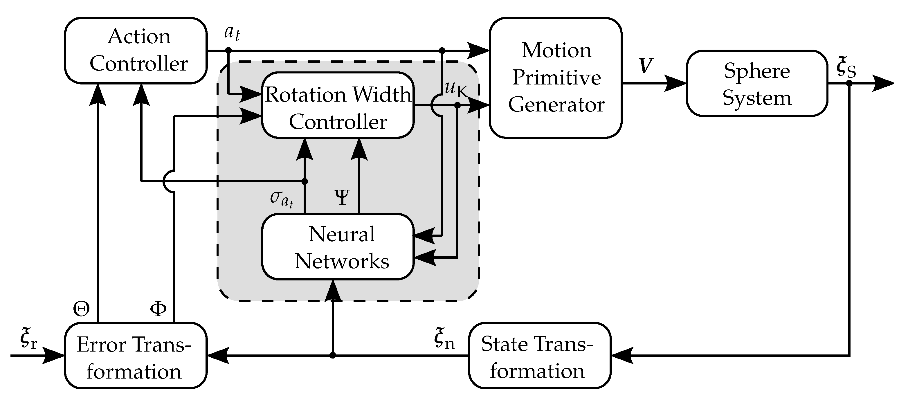
So far, we considered the mere impact driven motion. However, particularly for the sphere rotation, tangential friction between the beam and the sphere may have a large effect. In order to extend the previous generalized force formulation accordingly, we first derive the relative tangential velocity v t , k between the beam tip and the sphere surface, and subsequently use the Lagrange implementation described by Specker et al. [19].
Let us assume that the beam tip ξ T , k is in contact with the sphere. Then there is a point ξ P , k lying on the sphere with the same coordinates ξ T , k = ξ P , k . Since both points lie on different bodies, however, their velocities are computed differently. The beam tip velocity can again directly be computed from (31), while ξ ˙ P , k is derived similar to (34), i.e.,
ξ ˙ P , k = ξ ˙ S + I ω × r SP , k = ξ ˙ S + I A S ( S ω × S r SP , k ) = ξ ˙ S I A S S R SP , k S ω ,
where the cross product was replaced by a multiplication with the matrix
S R SP , k = 0 z SP , k y SP , k z SP , k 0 x SP , k y SP , k x SP , k 0
resulting from the vector
S r SP , k = x SP , k y SP , k z SP , k = S A I ( ξ P , k ξ S ) = S A I ( ξ T , k ξ S )
from the sphere center to the contact point in body frame coordinates. The relative velocity is then given by
v r , k = ξ ˙ P , k ξ ˙ T , k ,
which can be split up into two parts: The velocity v , k perpendicular to the sphere surface, and the tangential velocity v t , k . The perpendicular part is obtained by mapping v r , k onto the unit vector
e TS , k = x e , k y e , k z e , k = ξ S ξ T , k | ξ S ξ T , k |
pointing from the beam tip to the full sphere center, i.e.,
v , k = ( v r , k e TS ) e TS = E TS , k v r , k .
From the superposition principle it follows for the tangential velocity that
v t , k = ( I 3 × 3 E TS , k ) v r , k
with the 3 × 3 unit matrix I 3 × 3 . Given the friction velocity, it is now possible to define a dissipation function
D k = D v , k + D c , k + D s , k
depending on the absolute value | v t , k | , which include viscous ( D v , k ), Coulomb ( D c , k ), and Stribeck ( D s , k ) friction according to the definition in [19]:
D v , k = 0.5 d v | v t , k | 2
D c , k = μ c v c F BS , k log cosh | v t , k | v c
D s , k = d v v ^ s μ s μ c tanh v ^ s v c F BS , k v ^ s exp 0.5 0.5 | v t , k | v ^ s 2 .
For a detailed understanding of the origin of (46)–(48), we refer to [19]. It should be noted, however, that the coefficients d v , μ c , v c , μ s , and v ^ s can be chosen such that the corresponding friction force
F k D = D k | v t , k |
matches the setup. The generalized friction force vectors can then be computed by
Q B , k D Q ξ , k D S Q ω , k D = F k D | v t , k | q ˙ B , k | v t , k | ξ ˙ S | v t , k | S ω .
It remains to mention that the partial derivatives in (50) are problematic since any derivative of | v t , k | results in a singularity at zero. Therefore, Specker et al. [19] propose to approximate the absolute velocity by
| v t , k | ϵ + v t , k v t , k
with a small numeric stabilization variable ϵ > 0 .

4. Control Approach

In order to rotate the sphere according to a possibly time-dependent reference, consecutive kick and spin sequences are applied. Closed-loop control ensures that the motion converges to the desired rotation angles by choosing suitable inputs for the electrostatic actuators based on measurements of the current state. For the overall control design, we propose the following two-part approach. First, we aim to find suitable voltage signals for the electrostatic actuators to achieve a sphere rotation into the desired direction. Applying one of these predefined inputs results in a single kick motion, during which the sphere is transferred from one stable position into the next. These state transitions can now be understood as the discrete dynamics
x t + 1 = f ( x t , a t )
of a model with a higher abstraction level with state x t at discrete time step t. The dynamics define the next stable position after applying the discrete action a t A , e.g., a kick around the x- or y-axis, and we can choose from any action within the action set A that has been pre-calculated in the first step. The trajectories corresponding to each action can be seen as motion primitives, which are used e.g., in path planning algorithms for robots [28]. In the second step, we make use of this model to design a discrete closed-loop controller of the sphere angles, and finally extend the algorithm by a step width control for additional precision.

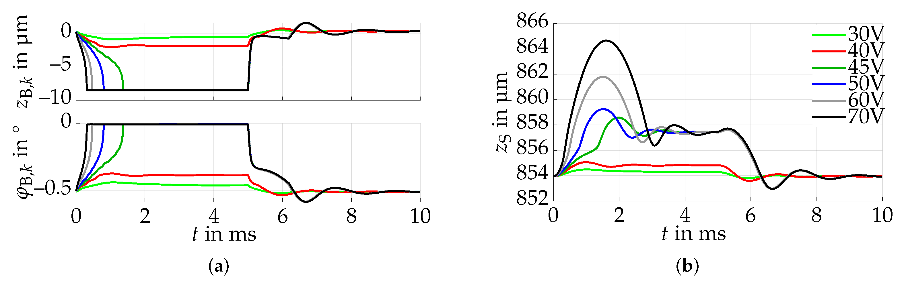
4.1. Step 1: Electrostatic Actuation

In order to choose the inputs for the electrostatic actuation, it is useful to understand the behavior of the beam-sphere interaction when applying a voltage to the actuators. Initially, the sphere is on top of the beam tips, which are bent downwards and are in contact with the insulated ground plate due to the sphere mass. If we now apply identical voltages to the actuators, the electrostatic forces pull the actuators’ rear ends in direction of the ground plate. Due to the leverage effect, the beam tips push the sphere upwards. Since the electrostatic forces increase quadratically with the voltage according to (7), the force transmitted to the sphere also becomes larger with higher inputs. This is shown in Figure 4. The parameter values used for this and the remaining simulations are given in Appendix A.3.
It can be seen that the kick intensity drastically increases between 40–45 V. This is due to the fact that the electrostatic force increases with decreasing plate distance, leading to instability for high voltages, which is called the pull-in. For the sake of completeness, note that this pull-in voltage changes when no sphere is placed on the beams, since lower forces are necessary to move the beams in that case.
To achieve a rotational sphere motion, different inputs have to be applied to the individual actuators. The goal is to find input voltages that achieve a maximum rotation in a predefined direction. Let us denote the single beam actuators as beams 1–4, starting with the left actuator and proceeding in a clockwise direction according to Figure 2b. The configuration suggests that applying identical voltages to two adjacent actuators will result in a diagonal rotation, e.g., actuating beams 1–2 will lead to a rotation from the hind left to the right front. Additionally, it may have a positive effect to use different voltages for the remaining two actuators. Suitable time courses of these inputs can be determined by numerical optimization.
In order to keep the number of optimization variables low and possibly allow for a simple implementation within the later hardware setup, we again use rectangular voltage pulses. Here, we use fixed amplitudes of 35 V and 80 V for each pair of actuators, where we defined 80 V to be the maximum voltage, and the lower voltage was found to be close to optimal by preliminary simulations. The inputs are then parameterized by the respective pulse width and the time delay between both positive voltage flanks. Next, these parameters are optimized using a genetic algorithm by maximizing the resulting rotation. As a result, we achieve an angular change of α 2 + β 2 = 0.54 in diagonal direction for a zero initial rotation of the sphere. The time course of the voltages, beam motion and resulting sphere rotation for this case are shown in Figure 5.
As can be seen, the sphere rotation is minimal during most of the actuation phase, and the actual rotatory motion starts at the first impact after the kick. This is not intuitive, since it was expected that the angular change is directly initiated by the pull-in motion of beams 3–4. Instead, this results in a translatory motion and the rotation results indirectly from the oblique impact with beams 1–2 during the negative voltage flank of V 3 , V 4 . This demonstrates not only the usefulness of the optimization, but also the importance of a mathematical model for preliminary analyses.
So far, we assumed that the initial state of the sphere corresponds to zero rotation angles, i.e., its center of gravity lies symmetrically in the center of the gap between the beam tips. It is now important to investigate the kick behavior for an initially deflected sphere. For evaluation purposes, we introduce a different representation of the rotational state than the Cardan angles. Since we are interested in the direction of the surface normal vector of the flat sphere part, we will use its x- and y-coordinates
x sn y sn = sin ( β ) cos ( β ) sin ( α )
to visualize the kick behavior. Now consider an initial rotation α = 20 , i.e., x sn = 0 , y sn = 0.342 . When we now apply the optimized inputs, neither the surface normal trajectory, nor its final state will lie on the diagonal 45 -line as it was the case before. This is depicted in Figure 6 and is, among others, a consequence of the displacement of the center of gravity, trying to converge to a state with zero rotation.
For a successful feedback controller design, it is useful to construct the discrete model (52) such that a specific action a t leads to a similar outcome, i.e., the same rotation direction and amplitude. While this may be achieved with considerable effort by optimizing the inputs for each possible initial sphere deflection, we found that a sufficient solution is given by increasing the voltage of a single beam such that the sphere motion in direction of the zero angle state is partially compensated. Due to the symmetry of the setup, it suffices to consider the initial states with y sn x sn and the kick from the hind left to the front right, since all other combinations result from either mirroring or rotating the state and actuated beams accordingly, as depicted in Figure 7.
Recall that assuming a kick from the hind left we applied V 1 = V 2 = 35 V and V 3 = V 4 = 80 V , which is the maximum voltage. To compensate for the sphere rotation in zero angle direction, we can add an offset v off to the voltage V 1 of the actuator on the right hand side when the surface normal directs into the upper right half-space, and V 2 in case of the lower left half-space. This offset depends on the initial sphere rotation and is found to be an approximately continuous function. In this work, we generated a grid of initial rotations and use the iteratively computed voltage offsets in terms of a lookup table. The effect of this offset is shown in Figure 8 for the same initial deflection as in Figure 6b. The actuator inputs derived in this section can now be summarized within the discrete action set A . The resulting discrete model can now be used for a feedback controller design.

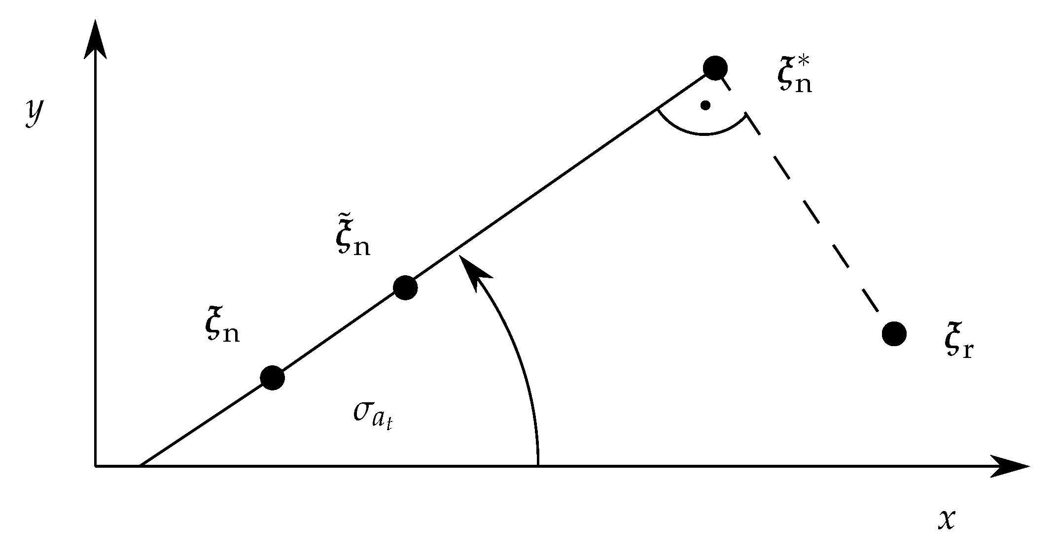
4.2. Step 2: Feedback Control

Given the discrete model derived in the previous section, we achieve rotations into pre-defined directions according to the chosen action. We now present a feedback controller, which subsequently selects from these actions, such that the sphere follows a time-variant reference rotation based on the error between the current and reference state. Let us first define the cartesian error vector
e x e y e z = ξ r ξ n
between the surface normal vector ξ n of the flat surface and the reference ξ r . In order to choose an action that reduces this error, it is beneficial to know the direction of the error, as well as the angular difference, i.e., the theoretically optimal kick direction and the absolute angle between the surface normal vectors. These can be described by the polar angle Θ [ 0 , 2 π ] of [ e x , e y ] and the absolute error angle Φ [ 0 , π ] given by
Φ = acos ( ξ n ξ r )
Θ = Θ ˜ e y 0 2 π Θ ˜ otherwise
Θ ˜ = acos e x e x 2 + e y 2 .
In general, Θ will not coincide with the actual kick direction, further denoted as σ t . Thus, we need to find a control law Π : Θ a t mapping each possible direction error to a discrete state. We here use the kick, which direction is closest to Θ , i.e.,
a t = arg min i | σ i Θ | .
So far, this control law excludes the possibility to remain in a certain position by not kicking the sphere at all. Especially since each kick has an overshoot with a transient oscillation, it may be reasonable to allow a small constant angular error Φ , instead of rotating the sphere when close to the reference. For this purpose, we apply (58) only when Φ is smaller than a design parameter Φ min .
This controller has two disadvantages: First, due to an approximately constant kick angle, the sphere will either oscillate around the desired state when Φ min is chosen to small, or will result in a steady state error otherwise. Secondly, even with high modeling effort, the hardware configuration can behave differently than the model due to the high complexity of the system, processing-related mechanical issues, and wear after some time of usage. As a result, the controller performance may be reduced. We therefore propose to extend the basic controller by a rotation width control to improve the actuator precision, and learning mechanisms to compensate for differences between the model and the actual actuator. The overall control loop is illustrated in Figure 9, in which the part shaded in gray corresponds to the extension explained in the remainder of this section.
Let us start with the adaption of the rotation width. So far, we assumed that the angular change per kick is fixed to the optimized value of approximately 0.54   . However, it is possible to adjust the kick intensity by suitably adapting the voltages applied to the electrostatic actuators. This has the advantage that both small and large angular changes are enabled, allowing for either precise rotations or fast angular velocities. Consider the case of a kick from the hind left, which we demonstrated in the previous section. We can achieve smaller rotation widths by reducing the voltages V 3 = V 4 = 80 V . This is shown in Figure 10 for initial states with α = 0 , 20 , 35 .
Besides the fact that we can achieve smaller rotation angles by adjusting the actuator voltages, the rotation width also decreases for larger sphere angles, and can even become negative. Let us assume that the characteristic Ψ = h a t ( V k ) is known. We can then achieve arbitrarily small angular changes by evaluating its inverse function, i.e., determining the necessary voltage for the desired rotation width. Since the exact characteristic of the setup is unknown and depends on the sphere state, as well as possible model uncertainty, we obtain this function by using an adaptive method. Note that we need such a function approximation for each kick action a t , hence the subscript. In the remainder of this work, we will moreover map the voltage V k to the intensity parameter u K [ 0 , 1 ] . As function approximators, we use neural networks given by
h a t ( u K ) = b a t + i = 1 n K w a t , i ζ i ( u K )
with bias b a t , weightings w a t = [ w a t , 1 , , w a t , n K ] , and the activation functions
ζ i ( u K ) = u K u K , i u K u K , i 0 otherwise .
This corresponds to a piecewise linear network with n K linear segments. It is important to understand that eventually, we will need an inverse expression u K = h a t 1 ( Ψ ) . However, during the process of learning the characteristic, we cannot guarantee that the function will always be injective, i.e., that a unique intensity parameter exists for a given rotation width. However, the piecewise linear function can efficiently be analyzed, finding a suitable intensity even if there is more than a single option or no option at all: In case the desired rotation Ψ * is larger than the maximum of h a t , the respective kick intensity of this maximum is used. Similarly, if smaller angles are necessary, the intensity corresponding to the minimum rotation width is applied. When there are several intensities leading to the identical result, the one needing the minimum voltage is used.
Now let us assume that h a t is known and we can evaluate the optimal intensity u K * if the desired rotation width Ψ * is given. It remains to compute this rotation from the current and reference state using the kick direction σ a t of the chosen action. Consider the following scenario depicted in Figure 11 in the x-y-plane.
Initially, the surface normal has the coordinates ξ n . By definition of the kick direction, the line between ξ n and any point ξ ˜ n resulting from a kick with intensity u K must enclose the angle σ a t with the x-axis. Assuming that σ a t is known, the ideal normal vector ξ n * closest to the given reference ξ r can be determined. It is then straightforward to compute the sphere rotation angle Ψ * necessary to reach ξ n * from ξ n , which completes the derivation of the adaptive rotation width.
As suggested before, the assumption of knowing σ a t may not be true due to model uncertainties, but it is necessary for both the basic controller, as well as the rotation width extension. Here, we solve this issue by also using an adaptive parameter σ a t for each kick direction. The learning procedure for this parameter and the neural networks can be described as follows: After each kick with intensity u K , compute both the actually achieved direction σ ˜ a t and the sphere rotation Ψ ˜ , which are then used to update the characteristics using
σ a t σ a t α σ ( σ a t σ ˜ a t ) ,
b a t b a t α b ( Ψ Ψ ˜ ) ,
w a t w a t α w ( Ψ Ψ ˜ ) h 1 ( Ψ ˜ ) w a t ,
with learning rates α σ , α b , α w . In summary, the optimal kick direction based on the angular deviation between the current state and the reference is chosen. Given the estimation of σ a t , the ideal rotation width is then computed, its corresponding kick intensity is obtained from the neural network and the kick is subsequently applied. The information from the kick is then used to update the adaptive parameters. This overall procedure is shown in Figure 12.

5. Results

We now want to demonstrate the performance of the control algorithm based on the derived mathematical model. We will first compare the basic non-adaptive controller with the extended version in a setpoint control, i.e., where the reference is constant, and then show their applicability to time-variant tracking problems. For the sake of computational time, we simulated the single kick trajectories for a grid of states and kick intensities beforehand, and use the discretized model in terms of a linearly interpolated lookup table. The simulations were realized with MATLAB ® [29] and the corresponding model parameters are given in Appendix A.3.

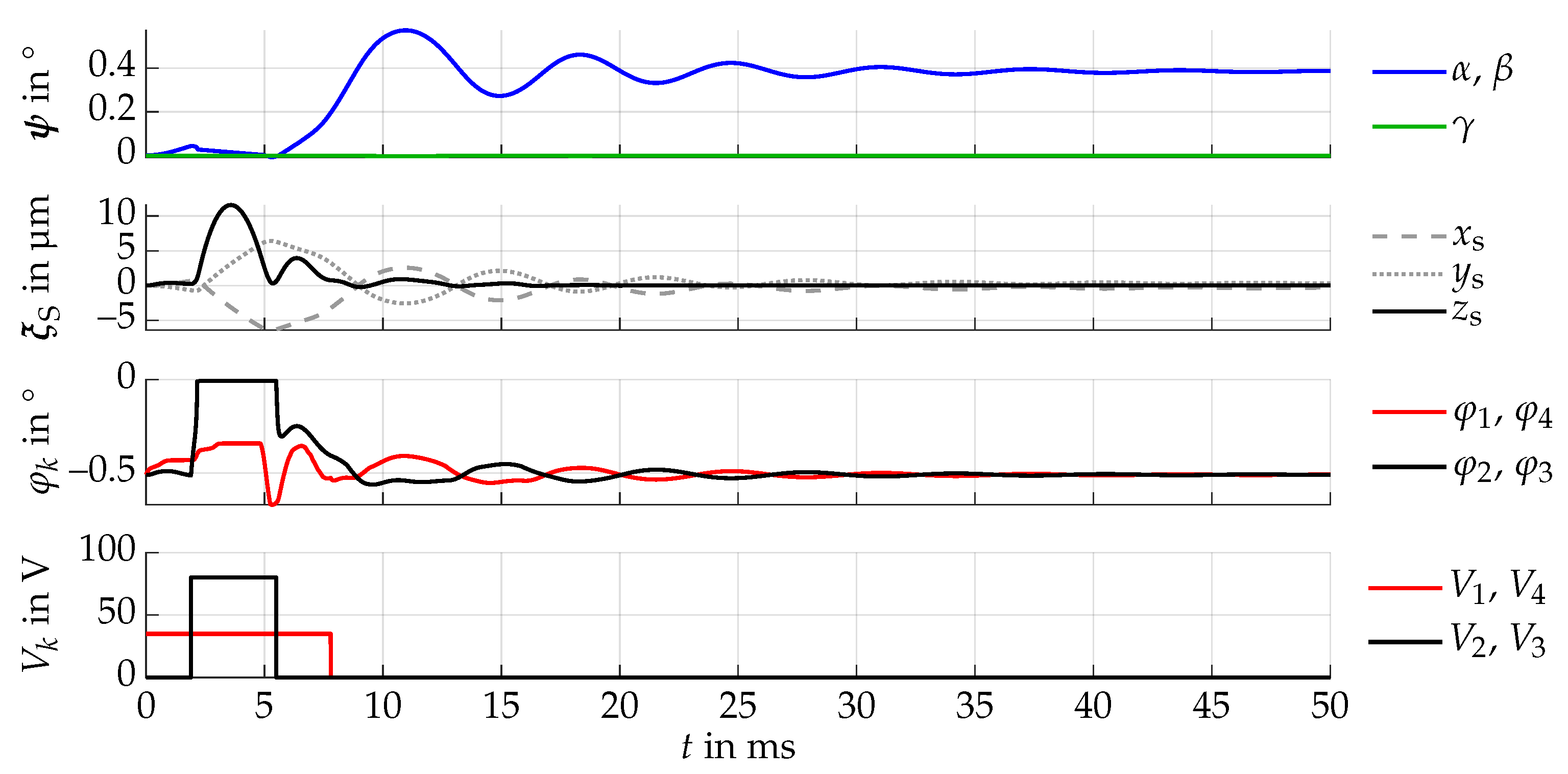
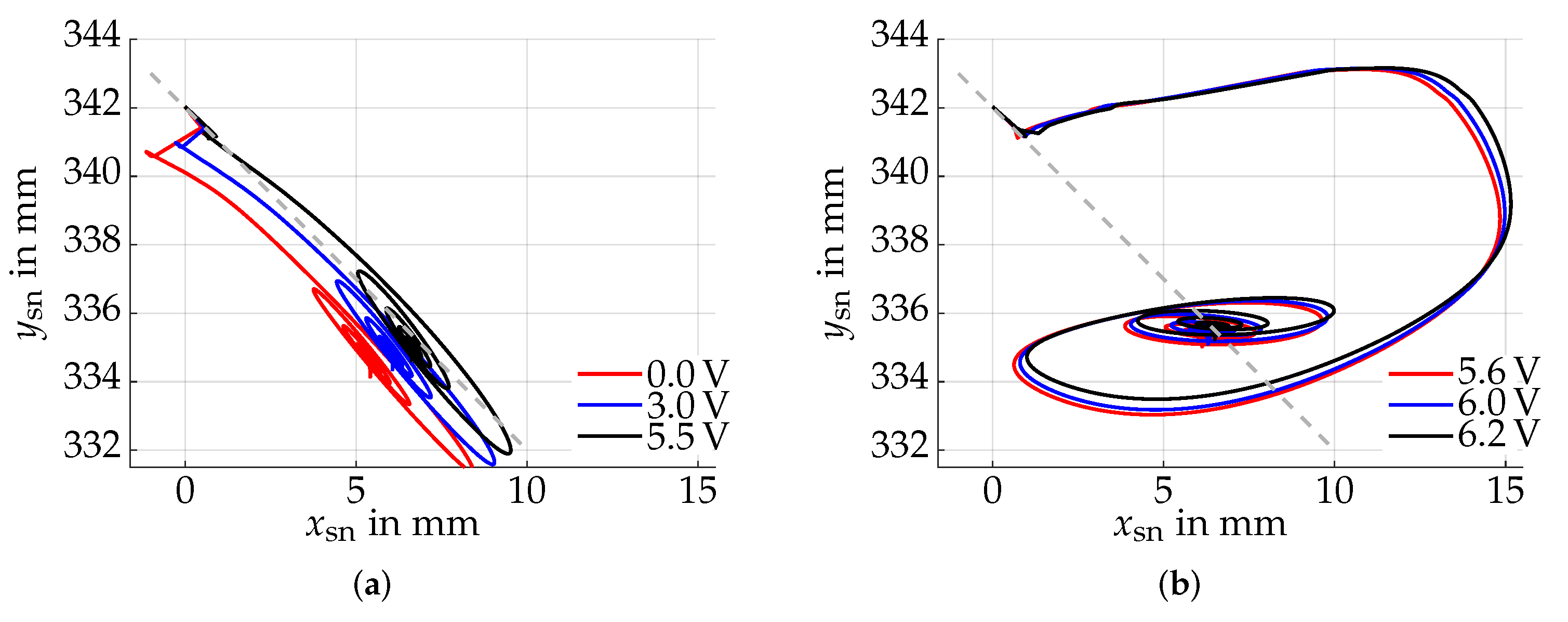
5.1. Setpoint Control

In this section, we will compare the behavior of both controllers when the objective is to reach a fixed state and remain in this resting position. Concerning the extended controller, we investigate the cases where the controller is simulated directly after the initialization and after a pre-learning phase. We assume that the spheres are initially in a state with zero rotation, and the reference surface normal vector has the coordinates ξ ref = [ 0.01 , 0.02 , 0.9997 ] . The result is seen in Figure 13.
As expected, the basic controller tends to oscillate for too small minimum resting angles Φ min , since the step width is too large for the error to get small enough. Enlarging this minimum angle, this oscillation disappears and a steady state error occurs. The trajectories with the extensions achieve high accuracy in only a few time steps. It is apparent, however, that these controllers cannot make use of their inherent advantages for larger minimum angles.
Besides the increased accuracy, one reason for the controller extension lies in its ability to adapt to model errors to some extend. In order to demonstrate this, we repeat the experiment, but with an error in the simulated system. In the simplest case, the kick directions do not correspond to the ideal ones. Here, we assume that each kick direction has an error of 12°. The trajectories are illustrated in Figure 14. For a larger Φ min , a similar result as in the previous case can be expected.
As before, the extended controllers show satisfactory results in terms of accuracy. It is interesting to see that the pre-learned controller seems to perform only slightly better than the one used with initialization parameters. However, the results visualized in this simulation study only show the terminal states after each kick, so that the transient behavior is not seen. If only the terminal state is important, the transient behavior may not be critical. Otherwise, it is important that the resting state is achieved using as few kicks as possible, which is only the case for the pre-learned controller. Moreover, it should be mentioned, that the basic controller is also able to achieve an acceptable behavior when being appropriately parameterized. Its advantage lies in the simplicity of its implementation, when no high accuracy is necessary.

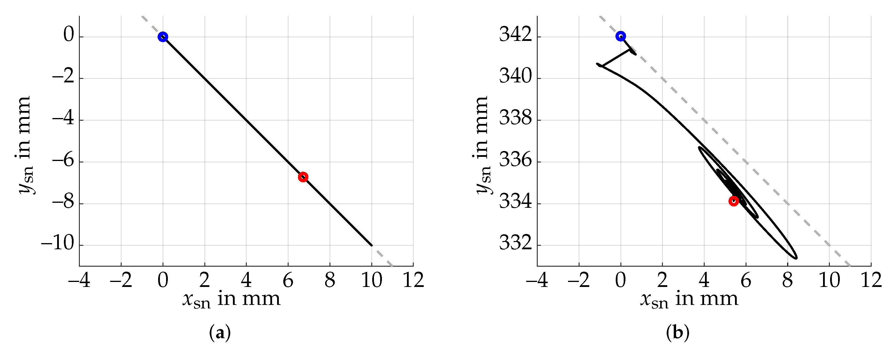
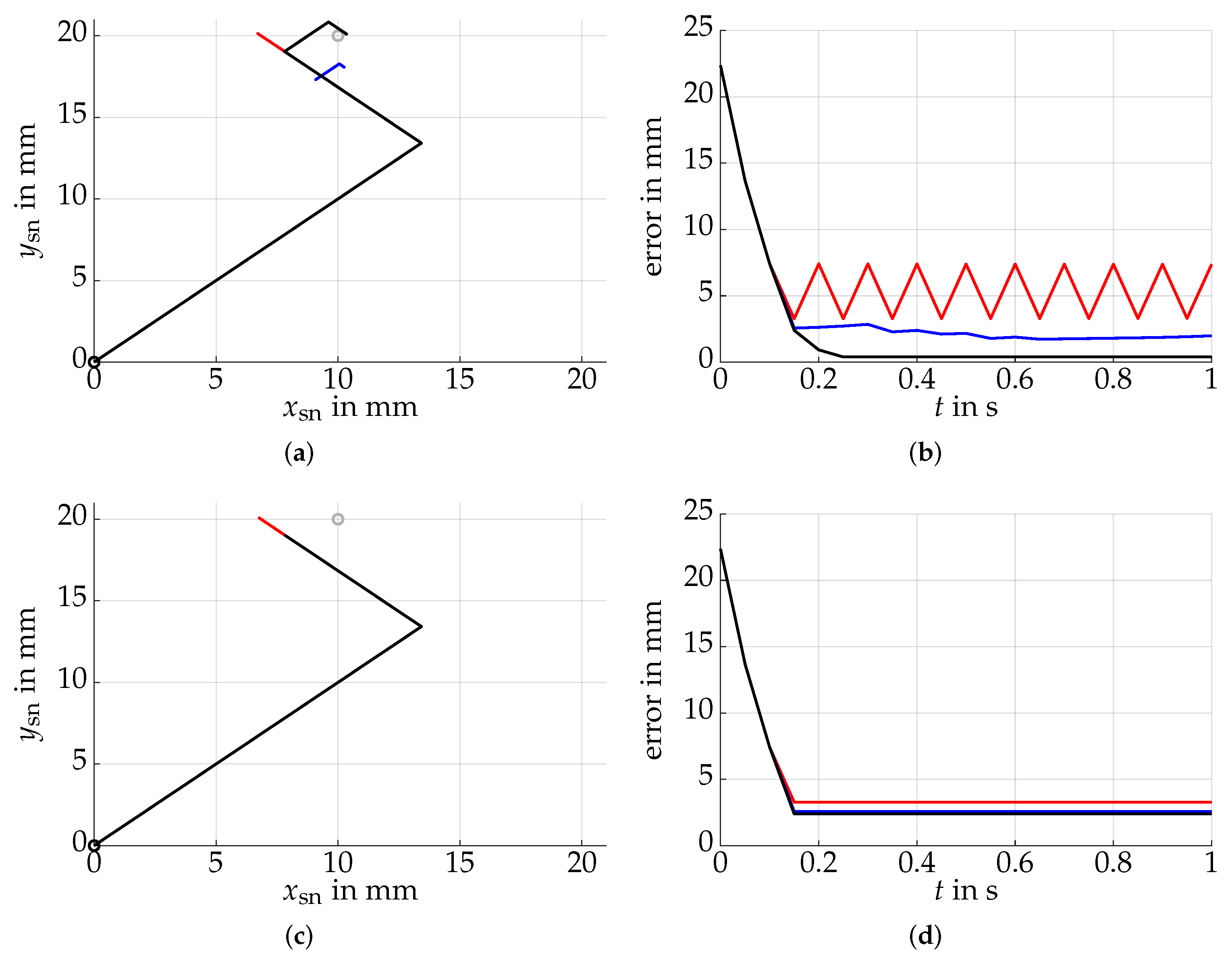
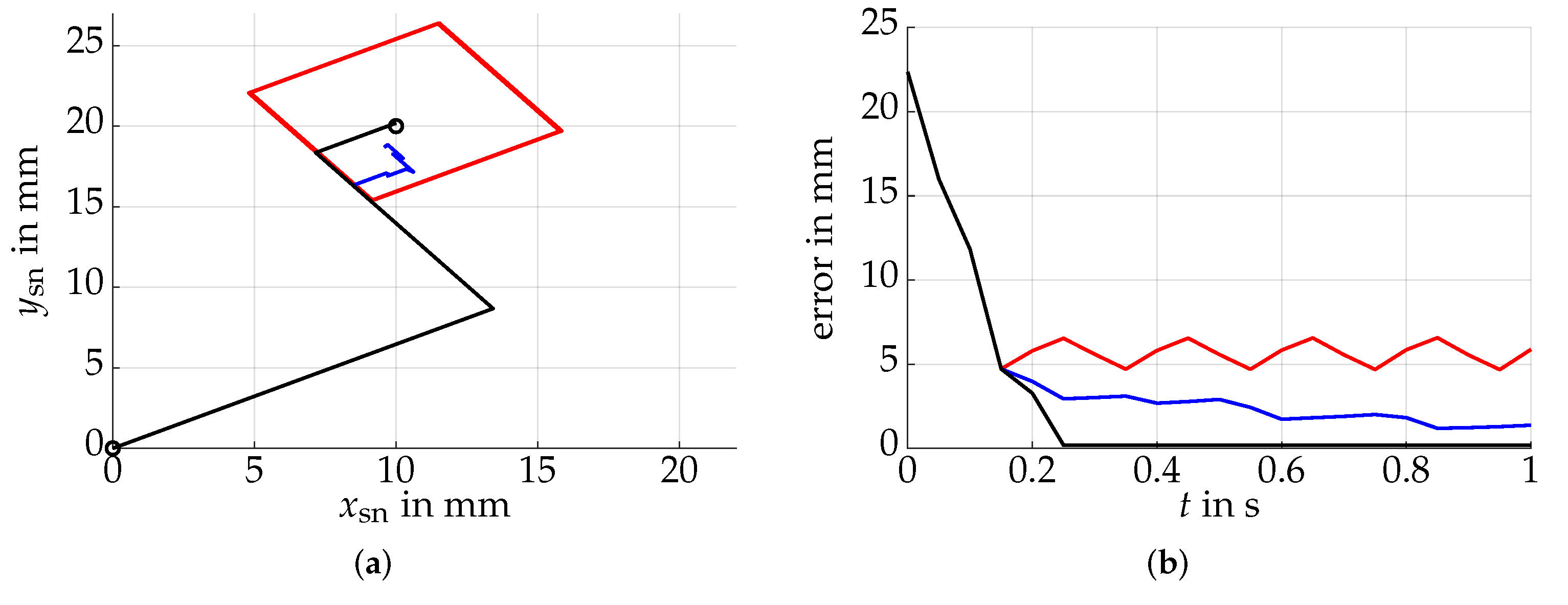
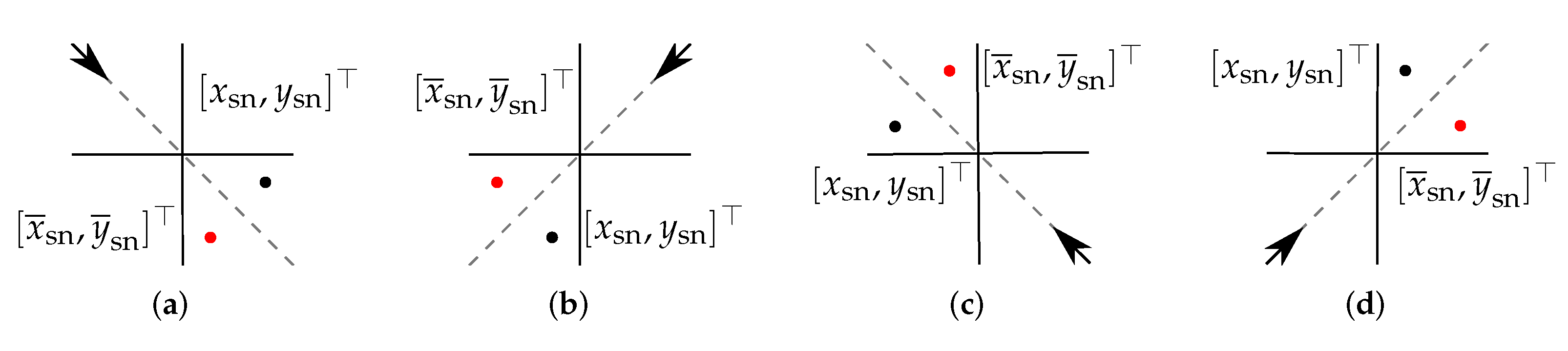
5.2. Trajectory Following Control

The setpoint control simulations have shown some advantages of the extended algorithms in terms of their steady state accuracy and their adaptability. In a second simulation, we now aim to analyze the behavior when the reference is a continuous function of time. The reference to be tracked is given in terms of x-, y coordinates by
x ref y ref = A max cos ( 2 π f 1 t ) cos ( 2 π f 1 t ) sin ( 2 π f 1 t ) ,
with A max = 0.44 and f 1 = 0.02 Hz . This function is designed to move within a large range of the state space. As before, we initialize the sphere to start with zero angles. Instead of simulating the ideal system behavior first, we directly use the perturbed system model, but with a mismatch of 33 kick direction. The results are visualized in Figure 15.
Both controllers show the ability to follow the trajectory with small errors, whereby the extended approach performs with a fifth of the basic controller error. Although both approaches may be reasonable choices, depending on the requirement on the controller, further studies on the limitations should be made to guarantee a satisfactory behavior. In case of the extended controller, a critical aspect is the rotation measurement quality, since this influences the ability to estimate the kick direction and rotation width characteristic.

6. Discussion

The presented micromirror can achieve large rotation angles due to the lack of restoring forces from springs. As a consequence, classical approaches for driving the mirror, which are based on fixed mechanical contacts, cannot be used. Instead, the rotation is achieved indirectly by applying inputs to electrostatic actuators, which in turn move the sphere by impacts and friction. The derived mathematical model can be understood as preliminary work used to study the complex mechanism and find suitable system inputs for later hardware experiments. It is important to mention that for such complex systems, we cannot assume perfect accordance with the real hardware setup, especially when using simplified system-level models. However, we expect that the general behavior coincides well enough, such that findings in simulation are transferable to the actual system to some extent. The advantage of such a model is its relatively low simulation time in contrast to more sophisticated approaches such as finite element modeling. For a successful comparison with a hardware setup, it will moreover be necessary to apply system identification to obtain optimal model parameters, which result in a dynamic behavior close to the actual micromirror. In the future, the model will therefore be compared to a hardware setup, and the results presented in this work have to be verified in experiment.
One of the main achievements corresponds to the optimized inputs maximizing the rotation angle, in combination with the perturbation of some actuator voltages, such that the sphere rotation direction is almost identical within the investigated state space of 40° rotation. This result is important, since it largely simplifies the controller design. Moreover, adapting the rotation width by reducing the applied voltages is a useful addition, allowing for precise motions. It is important to mention that for the ideal system, it is possible to reach any desired rotation angle without error. However, this may not be the case for the later hardware setup due to disturbances and measurement noise. Instead, it can be reasonable to remain in a certain position when the error is small enough, thus leading to a resolution of the specified error bound. The main problem of the current actuation principle lies in the oscillation of the sphere angle during and after the kick, which can in some cases be larger than the achieved final angular change. This is problematic if the mirror surface is supposed to transit smoothly between the resting states, as it may be the case for laser applications. Additionally, the maximum achievable angular velocity is limited by the fact that the oscillation has to stop before the next kick is applied. Both problems can be reduced by the implementation of active damping, e.g., by additional magnetic actuation. In the ideal case the oscillation can then be stopped at the point of its maximum rotation, i.e., shortly after applying the kick. This would lead to both larger angles and reduced transient times for each kick.
Faster angular velocities with less overshoot are also beneficial for the performance of the feedback controller. In this work, we described a control strategy which can adapt to model mismatch in terms of the kick direction. The advantage of this controller lies in its simple basic implementation and the extension to adapt the rotation width for increased precision. The capabilities of the approach were demonstrated in simulation in terms of setpoint control and trajectory following. So far, the controller could choose between four diagonal kick directions. These suffice to transfer the sphere in any rotational position. However, this results in a significantly slower motion for rotations in direction of the x- or y-axis, since two kicks are necessary for an exactly parallel motion. To overcome this, different input voltages need to be found, such that the sphere can directly be actuated in this direction. Its implementation within the control algorithm is then straight forward.
A possible issue of the presented configuration lies in the implementation of a free-lying sphere within practical applications, since the sphere is only held by its gravitational force. To increase this holding force, a permanent magnet below the setup may be used. During each kick and spin motion, this force can then be counteracted by additional electromagnetic solenoids.
Finally, it is necessary for a feedback controlled motion to measure the current state. A promising and cost-efficient method considers magnets below the actuator, and measuring the rotation via stray magnetic fields due to the flat side of the sphere. A challenge lies in the evaluation of these fields, as well as possibly high sensitivity due to magnetic disturbances. To reduce these effects, the use of state estimation algorithms like Kalman filters can be investigated.

7. Conclusions

In this work, we presented the system-level modeling approach for a novel microactuator, which achieves large deflection angles by rotating a freely moving, flattened sphere. The rotation is realized by impacts and friction with four electrostatic parallel plate actuators, where the pull-in effect is exploited to achieve the required forces. This results in a large variety of different multi-contact scenarios and leads to a complex relation between the actuator inputs and the sphere motion, which is challenging for both the modeling and control design approach. The contacts are considered within the model by a viscoelastic approximation, which is directly implementable within the Lagrange formulation. As a result, the complexity of the overall model is appropriately low to enable its use within numerical optimization methods for the determination of suitable inputs. For this purpose, sequences of system inputs maximizing the final rotation angle are found by a genetic algorithm. Based on the resulting motion primitives, an intuitive feedback controller design is proposed, such that the sphere follows a time-varying reference rotation. In order to take into account possible model uncertainty, and to increase the precision, the approach is extended by neural networks. The performance of the controller is evaluated in simulation, showing high accuracy even for initial model mismatch. In the future, a hardware configuration will be set up and the results of this work will be verified in experiment. In order to achieve a high level of agreement between the model and the hardware setup, system identification will be necessary to obtain the physical values for the model parameters.

Author Contributions

Conceptualization, C.A. and M.H.; methodology, M.O. and M.F.; software, M.O.; formal analysis, M.O.; investigation, M.O. and M.F.; writing—original draft preparation, M.O. and M.F.; visualization, M.O. and M.F.; supervision, C.A. and M.H.; funding acquisition, C.A. and M.H. All authors have read and agreed to the published version of the manuscript.

Funding

This research was funded by the German Research Foundation (DFG) within the priority program SPP2206 “KOMMMA”, project “Kick and Catch-Cooperative Microactuators for Freely Moving Platforms”.

Conflicts of Interest

The authors declare no conflict of interest.

Appendix A

Appendix A.1. Transformation Matrices

The transformation from the body frame of the sphere into the inertial frame is given by
I A S ( ψ ) = c β c γ c β s γ s β c α s γ + c γ s α s β c α c γ s α s β s γ c β s α s α s γ c α c γ s β c γ s α + c α s β s γ c α c β ,
where we abbreviated the sine and cosine functions of a variable x by s x = sin ( x ) and c x = cos ( x ) . The sphere angle derivatives ψ ˙ can be expressed as the rotation velocity vector S ω in sphere frame coordinates using the transformation matrix
ω T ψ ˙ ( ψ ) = c β c γ s γ 0 c β s γ c γ 0 s β 0 1 .

Appendix A.2. Sphere Inertia Tensor

Let the sphere have a flat surface enclosing an angle ϕ π with the center. The inertia tensor S J O regarding to the full sphere center is given by
S J O = ρ 0 π 0 2 π 0 r ( r r ) I 3 × 3 r r d x d ϑ d θ ρ 0 0.5 ϕ 0 2 π R ( ϕ , θ ) r ( r r ) I 3 × 3 r r d x d ϑ d θ
with the mass density ρ , lower integration bound R ( ϕ , θ ) = r cos ( 0.5 ϕ ) / cos ( θ ) , and the vector r = x [ sin θ cos ϑ , sin θ sin ϑ , cos θ ] . This results in
S J O = ρ Θ x x 0 0 0 Θ y y 0 0 0 Θ z z
with elements
Θ x x = Θ y y = 1 60 r 5 π cos ϕ / 2 + 1 2 16 9 cos ϕ / 2 3 + 18 cos ϕ / 2 2 17 cos ϕ / 2 ,
Θ z z = 8 15 r 5 π cos ϕ / 4 6 10 + 6 cos ϕ / 4 4 15 cos ϕ / 4 2 .
The inertia tensor S J S regarding to the center of gravity of the sphere can be computed using the parallel axis theorem, resulting in
S J S = S J O m S d cog 2 1 0 0 0 1 0 0 0 0 .

Appendix A.3. Simulation Parameters

Table A1. Design and simulation parameters used throughout the paper.
ParameterExplanationValue
z 0 Beam suspension position0 μm
d B Beam tip distance800 μm
L B Beam length1400 μm
w B Beam width200 μm
m B Beam mass96.695 μg
J B Beam inertia0.2665 g cm2
L cog Distance to beam center of gravity319 μm
L ES Capacitor plate length500 μm
w ES Capacitor plate width1300 μm
d Iso Virtual insulation layer thickness1.5 μm
k z Vertical beam spring stiffness35 N
k φ Rotational beam spring stiffness20 μN m
d B , z Vertical beam damping coefficient30 μN s
d B , φ Rotational beam damping coefficient5 nN m s
z G Ground plate position−10 μm
L G Ground plate length1000 μm
rSphere radius1000 μm
ϕ Sphere cutting angle90 °
m S Sphere mass30.973 mg
d cog Full sphere center and center of gravity distance49.7642 μm
d ω Rotational sphere damping coefficient0.1 nN m s
d ξ Translatory sphere damping coefficient5 mN s
k c Contact modeling parameter (linear stiffness) 5 × 10⁶
CContact modeling parameter (transition parameter) 0.25
r d Contact modeling parameter (impact loss parameter)10
d v Friction parameter (viscous friction) 0.05
μ c Friction parameter (Coulomb friction) 2
v c Friction parameter (Coulomb friction) 0.1
μ s Friction parameter (Stribeck friction) 0.5
v ^ s Friction parameter (Stribeck friction) 0.1
α σ Learning rate (kick direction) 0.9
α b Learning rate (neural network bias) 0.1
α w Learning rate (neural network weights) 0.1

References

  1. Holmström, S.T.S.; Baran, U.; Urey, H. MEMS Laser Scanners: A Review. J. Microelectromech. Syst. 2014, 23, 259–275. [Google Scholar] [CrossRef]
  2. Wang, Q.; Wang, W.; Zhuang, X.; Zhou, C.; Fan, B. Development of an Electrostatic Comb-Driven MEMS Scanning Mirror for Two-Dimensional Raster Scanning. Micromachines 2021, 12, 378. [Google Scholar] [CrossRef] [PubMed]
  3. Chong, J.; He, S.; Ben Mrad, R. Development of a Vector Display System Based on a Surface-Micromachined Micromirror. IEEE Trans. Ind. Electron. 2012, 59, 4863–4870. [Google Scholar] [CrossRef]
  4. Hu, F.; Yao, J.; Qiu, C.; Ren, H. A MEMS micromirror driven by electrostatic force. J. Electrost. 2010, 68, 237–242. [Google Scholar] [CrossRef]
  5. Jeong, H.M.; Park, Y.H.; Jeong, H.K.; Cho, Y.C.; Chang, S.M.; Kim, J.O.; Kang, S.J.; Hwang, J.S.; Lee, J.H. Slow scanning electromagnetic MEMS scanner for laser display. In MOEMS and Miniaturized Systems VII; SPIE: Bellingham, DC, USA, 2008; Volume 6887, pp. 41–52. [Google Scholar] [CrossRef]
  6. Liao, W.; Liu, W.; Zhu, Y.; Tang, Y.; Wang, B.; Xie, H. A Tip-Tilt-Piston Micromirror With Symmetrical Lateral-Shift-Free Piezoelectric Actuators. IEEE Sens. J. 2013, 13, 2873–2881. [Google Scholar] [CrossRef]
  7. Makishi, W.; Kawai, Y.; Esashi, M. Magnetic torque driving 2D micro scanner with a non-resonant large scan angle. In Proceedings of the TRANSDUCERS 2009–2009 International Solid-State Sensors, Actuators and Microsystems Conference, Denver, CO, USA, 21–25 June 2009; pp. 904–907. [Google Scholar] [CrossRef]
  8. Weinberger, S.; Nguyen, T.; Lecomte, R.; Cheriguen, Y.; Ament, C.; Hoffmann, M. Linearized control of an uniaxial micromirror with electrostatic parallel-plate actuation. Microsyst. Technol. 2015, 22, 441–447. [Google Scholar] [CrossRef]
  9. Bunge, F.; Leopold, S.; Bohm, S.; Hoffmann, M. Scanning micromirror for large, quasi-static 2D-deflections based on electrostatic driven rotation of a hemisphere. Sens. Actuators Phys. 2016, 243, 159–166. [Google Scholar] [CrossRef]
  10. DFG, Kick and Catch-Cooperative Microactuators for Freely Moving Platforms: SPP 2206: Cooperative Multilevel Multistable Micro Actuator Systems (KOMMMA). Available online: https://gepris.dfg.de/gepris/projekt/424616052 (accessed on 6 March 2022).
  11. Barjuei, E.; Caldwell, D.; Ortiz, J. Bond Graph Modeling and Kalman Filter Observer Design for an Industrial Back-Support Exoskeleton. Designs 2020, 4, 53. [Google Scholar] [CrossRef]
  12. Kumbhar, S.; Sudhagar, P.; Desavale, R. An overview of dynamic modeling of rolling-element bearings. Noise Vib. Worldw. 2021, 52, 1–16. [Google Scholar] [CrossRef]
  13. Pustan, M.; Paquay, S.; Rochus, V.; Golinval, J.C. Modeling and finite element analysis of mechanical behavior of flexible MEMS components. Microsyst. Technol. 2011, 17, 553–562. [Google Scholar] [CrossRef]
  14. Schütz, A.; Olbrich, M.; Hu, S.; Ament, C.; Bechtold, T. Parametric system-level models for position-control of novel electromagnetic free flight microactuator. Microelectron. Reliab. 2021, 119, 1–9. [Google Scholar] [CrossRef]
  15. Yerlikaya, U.; Balkan, R. Dynamic modeling and control of an electromechanical control actuation system. In Proceedings of the Dynamic Systems and Control Conference, Tysons, WV, USA, 11–13 October 2017; pp. 1–10. [Google Scholar] [CrossRef]
  16. Hurmuzlu, Y.; Marghitu, D. Rigid Body Collisions of Planar Kinematic Chains with Multiple Contact Points. Int. J. Robot. Res. 1994, 13, 82–92. [Google Scholar] [CrossRef]
  17. Popov, V.; Heß, M. Method of dimensionality reduction in contact mechanics and friction: A users’ handbook. Facta Univ. 2014, 12, 1–14. [Google Scholar]
  18. Fischer-Cripps, A. The Hertzian contact surface. J. Mater. Sci. 1999, 34, 129–137. [Google Scholar] [CrossRef]
  19. Specker, T.; Buchholz, M.; Dietmayer, K. Dynamical Modeling of Constraints with Friction in Mechanical Systems. In Proceedings of the 8th Vienna International Conference on Mathematical Modelling, Vienna, Austria, 18–20 February 2015; pp. 514–519. [Google Scholar] [CrossRef]
  20. Potocnik, B.; Music, G.; Zupancic, B. Model predictive control systems with discrete inputs. In Proceedings of the 12th IEEE Mediterranean Electrotechnical Conference, Dubrovnik, Croatia, 12–15 May 2004; Volume 1, pp. 383–386. [Google Scholar] [CrossRef]
  21. Asok, R.; Jinbo, F.; Constantino, L. Optimal supervisory control of finite state automata. Int. J. Control 2004, 77, 1083–1100. [Google Scholar] [CrossRef]
  22. Konaka, E. Controller design for discrete input control system based on machine-learning. In Proceedings of the SICE Annual Conference 2011, Tokyo, Japan, 13–18 September 2011; pp. 601–604. [Google Scholar]
  23. Glorennec, P.Y. Reinforcement learning: An overview. In Proceedings of the European Symposium on Intelligent Techniques, Aachen, Germany, 14–15 September 2000; pp. 14–15. [Google Scholar]
  24. Zhou, W.; Lan, H.; Yu, H.; Lai, L.; Peng, B.; He, X. Consideration of the fringe effects of capacitors in micro accelerometer design. Trans. Inst. Meas. Control 2018, 40, 1881–1996. [Google Scholar] [CrossRef]
  25. Feng, Y.; Zhou, Z.; Wang, W.; Rao, Z.; Han, Y. The 3D Capacitance Modeling of Non-parallel Plates Based on Conformal Mapping. In Proceedings of the 16th IEEE International Conference on Nano/Micro Engineered and Molecular Systems, Xiamen, China, 25–29 April 2021; pp. 1264–1267. [Google Scholar] [CrossRef]
  26. Awrejcewicz, J.; Koruba, Z. Classical Mechanics: Applied Mechanics and Mechatronics; Springer Science & Business Media: Berlin/Heidelberg, Germany, 2012; Volume 30. [Google Scholar] [CrossRef]
  27. Olbrich, M.; Schütz, A.; Bechtold, T.; Ament, C. Design and Optimal Control of a Multistable, Cooperative Microactuator. Actuators 2021, 10, 183. [Google Scholar] [CrossRef]
  28. Dharmadhikari, M.; Dang, T.; Solanka, L.; Loje, J.; Nguyen, H.; Khedekar, N.; Alexis, K. Motion Primitives-based Path Planning for Fast and Agile Exploration using Aerial Robots. In Proceedings of the 2020 IEEE International Conference on Robotics and Automation (ICRA), Paris, France, 31 May–31 August 2020; pp. 179–185. [Google Scholar] [CrossRef]
  29. The MathWorks Inc. MATLAB (R2019a); The MathWorks Inc.: Natick, MA, USA, 2019. [Google Scholar]
Figure 1. (a) Resting position: The sphere remains in stable rest position. (b) Kick and spin actuation: The sphere is transferred into a free flight phase, while a torque is transmitted to set it in rotation by asymmetric actuation. (c) Flight phase: The sphere is not in contact with the beams and rotates freely into the desired direction. (d) Catch and resting: The sphere lands in a deflected position and is kept in a stable position.
Actuators 11 00090 g001
Figure 2. System parameters used for the derivation of the motion equations. (a) Side view of the actuator illustrating the sphere, movable beam, and ground plates parameters. The gray parts correspond to the electrical contacts. (b) Top view of the electrostatic beams without sphere. The beams are symmetrically arranged and the respective rotations around the z-axis are described by parameters δ k , k = 1 , , 4 . The parts shaded in gray illustrate the dimensions of the parallel plate actuators’ electrical contacts.
Actuators 11 00090 g002
Figure 3. Definition of the overlap between the ground plate and the beam. (a) A virtual insulation layer with thickness d Iso (red) is used for numerical stability, preventing a short circuit within the simulation in case of an overlap. Since no contact occurs, the distances s R , k and s F , k are positive. (b) The front part of the beam is in contact with the ground plate, resulting in s F , k < 0 .
Actuators 11 00090 g003
Figure 4. Model-based simulation of the beam and sphere motion when applying rectangular voltage pulses with amplitudes between 30–70 V to all beams. After 5 ms, the input is reduced to zero. (a) The electrostatic force pulls the actuator beam downwards (top figure). Due to the leverage effect at the front end of the ground plate, the beam angle increases (bottom figure). For voltages larger than 44 V a pull-in occurs, leading to a fast kick motion. (b) The upwards motions of the beam tips result in a change in the z-position of the sphere. For high voltages, a flight phase of the sphere is achieved.
Actuators 11 00090 g004
Figure 5. The optimized rectangular voltages (bottom) are applied to the actuators, resulting in a delayed pull-in motion for beams 2–3 (second last). Due to this force, the sphere is kicked upwards, drifting into the hind left (second). The sphere rotation (top) is then induced by a complex combination of the impact with beams 1–2 as well as releasing beams 3–4 from the pull-in. After a settling time of approximately 50 ms, the sphere achieves a diagonal rotation of α = β = 0.39 .
Actuators 11 00090 g005
Figure 6. Trajectory of the surface normal vector when applying the optimized inputs for spheres with different initial angles. The desired direction corresponds to a 45 -line (dashed). (a) The sphere is initialized with zero angles (blue circle) and the surface normal trajectory lies on the line of the desired direction. The final deflection corresponds to 0.54 (red circle). (b) Applying the same inputs for an initial rotation of α = 20 (blue circle) leads to an additional motion in the direction perpendicular to the 45 -line. The final state is marked by a red circle.
Actuators 11 00090 g006
Figure 7. Exploitation of the symmetry in terms of the surface normal coordinates. (a) Applying a kick from the hind left (depicted as arrow) with current state [ x sn , y sn ] (black dot) leads to the identical motion as for a state [ x ¯ sn , y ¯ sn ] , mirrored at the diagonal axis (red dot). (bd) The same relative behavior is obtained when the state and kick direction are rotated and mirrored accordingly. Thus, all combinations of states and kick directions can be determined, given the motion of each state within the upper right half-space when applying a kick from the hind left is known.
Actuators 11 00090 g007
Figure 8. Effect of the voltage offset v off for beam 1 for an initial deflection of α = 20 . The goal is to achieve a resulting rotation direction of 45 (dashed line). (a) A voltage offset up to 5.5 V reduces the rotation direction error with small oscillation in its perpendicular direction. (b) A further increase of the voltage up to approximately 6.2 V leads to a change in the overall behavior, including larger oscillations in undesired directions, but achieves higher accuracy of the final state.
Actuators 11 00090 g008
Figure 9. Block diagram of the basic control loop (white background) and an extension for higher precision (gray background). The measured sphere state ξ S is transformed into surface normal coordinates ξ n , and its deviation from the reference coordinates ξ r is transformed into angular errors Θ , Φ . The action controller then chooses a suitable action a t , based on which the motion primitive generator computes the corresponding input sequences V for the beam actuators. The extension consisting of neural networks and a rotation width controller enable an improved angular resolution.
Actuators 11 00090 g009
Figure 10. Rotation width for different beam voltages for initial deflections α = 0 , 20 , 35 . This can be used to obtain a higher accuracy. The rotation width slightly decreases with larger initial rotation of the sphere.
Actuators 11 00090 g010
Figure 11. Starting with normal vector ξ n and kick direction σ a t , any point ξ ˜ n lying on the line can be reached by a sufficient kick intensity. The goal is to find the optimal kick intensity to reach ξ n * , which is closest to the reference ξ r .
Actuators 11 00090 g011
Figure 12. Outline of the control algorithm combining adaptive direction parameters and neural networks for the rotation width control.
Actuators 11 00090 g012
Figure 13. Trajectories (left) from the zero rotation state (black circle) to the reference (gray circle) and the respective errors (right) for the basic (red), extended (blue), and pre-learned extended (black) controllers. The minimum angle Φ min is 0.05 on the top and 0.25 on bottom. (a) While the basic controller is not able to achieve a steady state due to a too small Φ min , the extended controllers achieve high accuracies with fewer time steps. (b) The quadratic errors confirm the expectation of an oscillating basic controller and show the advantage of the extension. (c) If Φ min is larger, the controllers converge to similar solutions. (d) A larger minimum angle leads to higher steady state errors, but improves the basic controller due to the missing oscillation. The advantages of the extension do not take effect.
Actuators 11 00090 g013
Figure 14. The basic (red), extended (blue), and pre-learned extended (black) controllers are now applied to the same setpoint problem, but the kick directions do not coincide with those of the ideal model (a) The basic controller now oscillates in two dimensions, while the extended controllers quickly adapt to the new kick directions. (b) The error decreases slower than in case of the ideal model for all controllers, but a similar number of steps is needed for the extended controllers to converge to the desired position.
Actuators 11 00090 g014
Figure 15. Following of a time-dependent reference trajectory using a simulation system with different kick direction than the model. The tracking errors correspond to the quadratic x-y-deviation of the surface normal vector from the reference. (a) The best result of the basic controller (left) is compared with the extended one (right). Although the basic controller is not able to learn the deviating kick direction, its result is comparable to that of the extended controller. (b) The quadratic errors between the trajectories deviate by a factor of approximately 5, showing that the extended controller is more accurate.
Actuators 11 00090 g015
Publisher’s Note: MDPI stays neutral with regard to jurisdictional claims in published maps and institutional affiliations.

