Abstract
With the diversification of robots, modularization of robots has been attracting attention. In our previous study, we developed a robot that mimics the principle of human joint drive using a straight-fiber-type pneumatic rubber artificial muscle (“artificial muscle”) and a magnetorheological fluid brake (“MR brake”). The variable viscoelastic joints have been modularized. Therefore, this paper evaluates the basic characteristics of the developed Joint Module, characterizes the variable viscoelastic joint, and compares it with existing modules. As basic characteristics, we confirmed that the Joint Module has a variable viscoelastic element by experimentally verifying the joint angle, stiffness, viscosity, and tracking performance of the generated torque to the command value. As a characteristic evaluation, we verified the change in motion and response to external disturbances due to differences in driving methods through simulations and experiments and proved the strength of the variable viscoelastic joint against external disturbances, which is a characteristic of variable viscoelastic joints. Based on the results of the basic characterization and the characterization of the variable viscoelastic drive joint, we discussed what kind of device the Joint Module is suitable to be applied to and clarified the position of the variable viscoelastic joint as an actuator system.
1. Introduction
A wide range of robots have been developed in recent years [1,2,3]. Robots are used in a variety of fields, including factory production lines, human power assistance, and human-to-human communication. Existing robots, in contrast, are not widely used in many fields due to their limited versatility and high cost. We believe that robot modularization is an effective way to enable robots to be used in a broader range of applications. Modularization simplifies the design and maintenance of robots while also lowering the cost of manufacturing and operation. Existing modules are driven mainly by motors and reduction gears, and the structure includes a drive and control unit. In addition, there are hydraulic modules that have hydraulic pistons and valves and a control unit.
Previous research has looked into variable viscoelastic joints using straight-fiber-type pneumatic rubber artificial muscles (hereafter referred to as artificial muscles) and magnetorheological fluid brake (hereafter referred to as MR brake) [4]. Artificial muscles are arranged in an antagonistic pattern in this joint, and an MR brake is used. The artificial muscles are lightweight, powerful and have variable elasticity, whereas the MR brake is light, has a quick response time of a few tens of milliseconds, and achieves apparent variable viscosity by controlling the brake force [5]. Variable viscoelastic properties are achieved by combining these two devices. The MR brake is used as a friction brake in the variable viscoelastic drive joint to accumulate the potential energy of the artificial muscles, and then the brake is released instantly to obtain instantaneous force. Artificial muscles are structurally soft and resistant to impact forces because they are used as actuators. Furthermore, because artificial muscles have a high-power density, a compact and lightweight device with high power can be created. In previous research, we created a throwing robot with instantaneous power [5] and a wearable assistive suit with lightweight and high power [6] based on these characteristics. The variable viscoelastic drive joint is structurally more human-like than traditional motor-driven robots because it mimics the human joint drive principle. As a result, we believe that the variable viscoelastic drive joints can be used to create a robot capable of coexisting with humans cooperatively.
As previously stated, there are numerous fields wherein existing robots have not been widely utilized. According to the Ministry of Economy, Trade and Industry [7], the robot industry’s market size is expected to grow in the future, and the market is expected to expand in fields other than manufacturing. As a result, it is expected that there will be a high demand for robots in the future, particularly in the field of human–robot collaboration. As a result, we anticipate that variable viscoelastic drive joints, in addition to motors, will be used in more applications. In contrast, existing robots that use variable viscoelastic joints have a problem with narrow environment adaptation and high design and operation costs. As a result, it is critical to demonstrate the versatility of variable viscoelastic joints to apply them to a broader range of fields.
In this research, we aim to improve the versatility of variable viscoelastic drive joints by creating a variable viscoelastic Joint Module (hereafter referred to as “Joint Module”).
Previous research has shown that the Joint Module depicted in Figure 1 can be developed and its joint stiffness can be varied [8]. The Joint Module is developed in this paper, and the basic characteristics of the developed Joint Module are measured. We also compare the Joint Module to existing modularized robots (hereafter referred to as “modular robots”) to better understand the characteristics of the Joint Module.
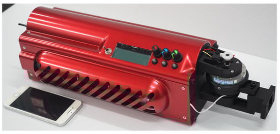
Figure 1.
Picture of variable viscoelastic Joint Module.
In this paper, the concept of modularization of the device is described in Chapter 2. In Chapter 3, we describe the outline of the developed Joint Module. Chapter 4 describes the basic characteristics evaluation experiment of the Joint Module and its results and discussion. Chapter 5 describes the performance evaluation experiment of the Joint Module, its response to disturbance and its results and discussion. In Chapter 6, we compare the performance of the Joint Module with existing modules. In Chapter 7, based on the performance of the Joint Module evaluated in Chapters 4 and 5, we propose an application example of the Joint Module. Finally, Chapter 8 concludes the paper.
The contribution of this paper is shown below.
- A variable viscoelastic Joint Module containing a pneumatic pressure source was developed.
- The basic characteristics evaluation experiment of the Joint Module confirmed that the Joint Module has a variable viscoelastic element.
- Performance evaluation experiments using the Joint Module proved that it is resistant to external disturbances, which is one of the characteristics of variable viscoelastic joints.
- The position of the variable viscoelastic joint as an actuator system was clarified.
2. Concept of the Device Developed
2.1. Modularization of Variable Viscoelastic Devices
Modularization is defined by Jose Baca et al. [9] as “the division of a complex system into elements with high portability, ease of maintenance, and logical clarity.” The following five, benefits of modularization, according to Yisheng Guan et al. [10], can be expected:
- Versatility: New robotic systems can be quickly built, or new functionalities can be enabled by connecting a few identical or similar modules in different configurations. As a result, they can adapt to various tasks and environments;
- Reconfigurability: The configuration (mechanical structure) of a modular robot may be modified from one type to another by changing the connection or combination of modules automatically or manually;
- Scalability: A robot’s degree of freedom can be increased or decreased simply by adding or removing joint modules from the system;
- Low costs: The modules are usually identical and may be mass-produced. The costs of design, manufacture, assembly, and maintenance of systems consisting of modules are much less than those of conventional systems with the same function;
- Fault tolerance: If a module is found to malfunction, it can be replaced with another in a matter of seconds by disconnecting and reconnecting them.
Based on the above, we set the following goals for the Joint Module to be developed in this research:
- The device can be driven cordlessly without using an external system such as a household power supply;
- The weight of one Joint Module should be less than 4 kg;
- Multiple joint modules can be used in combination.
2.2. Variable Viscoelastic Joint
The driving principle of the variable viscoelastic joint used in this study is depicted in Figure 2. The joint is made up of a pair of artificial muscles that are antagonistically arranged and an MR brake, which mimics the human joint drive principle. By applying air pressure to the artificial muscles, the joint’s elasticity can be varied. The MR brake is connected to the output shaft, and the frictional torque of the MR brake is controlled according to the angular velocity of the output shaft to realize the variable viscosity of the joint.
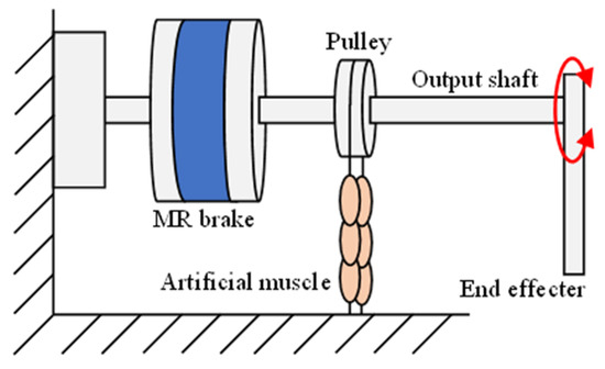
Figure 2.
Operation principle of variable viscoelastic joint.
2.3. Feedforward Controller (FFC)
Here, feedforward control (abbreviated FFC) [11] is described, which controls the joint torque, angle, stiffness, and viscosity of a single joint.
First, the method for controlling the joint torque, angle, and stiffness in a single joint is described. By applying air pressure to the artificial muscle placed antagonistically. The device joint angle and stiffness were independently controlled. Furthermore, we estimated the joint torque and control the applied pressure of the artificial muscle. Table 1 shows the parameters considered in this section. The contraction force F of the artificial muscle alone can be expressed by Equation (1) by the applied pressure P and the contraction amount x of one segment.

Table 1.
Parameter of the viscoelastic joint.
G1(xi), G2(xi), and G3(xi) are determined from the shape of the artificial muscle. Furthermore, i = 1 and 2 symbolize each artificial muscle. Here, an experimental identification model is introduced [11]. G3(xi)/G2(xi) and −G1(xi)/G2(xi) are approximated by a(xi) and b(xi) in Equations (2) and (3), respectively, and Equation Expressed as (4).
The parameters identified in the experiment, c, d, f, and g are the intrinsic constants of each artificial muscle and are given in Equations (2) and (3). The spring constant ki of the artificial muscle is determined by the applied pressure Pi and the contraction amount xi as shown in Equations (5) and (6).
However, kaai and kabi are intrinsic constants of each artificial muscle.
Based on the mechanical equilibrium and geometric constraint between the pulley and the arm at the joint where the two artificial muscles shown in Figure 3 are antagonistically arranged, applying Equations (2)–(6) yields the applied pressure to each artificial muscle as Equations (7) and (8).
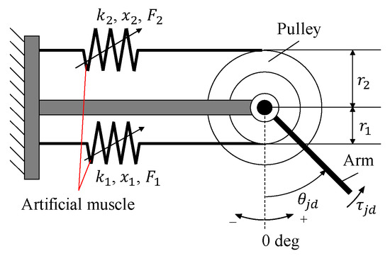
Figure 3.
The model of the viscoelastic joint. This joint can obtain any joint angle and joint stiffness by controlling the air pressure applied to the artificial muscle.
The contraction amount of each artificial muscle at that time is given by Equations (9) and (10). The subscripts 1 and 2 represent artificial muscles 1 and 2, respectively
From Equations (7)–(12), the air pressures P1 and P2 applied to the artificial muscles are obtained from the joint torque τjd, angle θjd, and stiffness Kjd. Furthermore, the angle θjd and the stiffness Kjd can be controlled independently, and the joint torque τjd can then be estimated.
Following this process, the method for controlling joint viscosity in a single joint is explained. Assuming that the friction torque of the MR brake is τy, the angular velocity is dθ/dt, and the joint viscosity is Djd, the relationship described by Equation (11) holds.
This is used to control the joint viscosity by determining the friction torque.
Figure 4 depicts the FFC’s block diagram, which controls the joint torque, angle, stiffness, and viscosity.
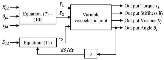
Figure 4.
The block diagram of the feed-forward controller.
3. Overview of Variable Viscoelastic Joint Module (Joint Module)
The appearance of the developed Joint Module is depicted in Figure 1, and the 3D CAD model is shown in Figure 5. The developed Joint Module is made up of a drive unit, a pneumatic system, a control unit, an electric system, a sensor, and an interface. When the pneumatic tank is full, its dimensions are 448 × 180 × 127 mm, and its weight is 3.14 kg. A variable viscoelastic drive joint is used for the drive. This joint has an antagonistic arrangement of artificial muscles, and the MR brakes are used in the joints. The rigidity of the joint and the angle of the drive arm are controlled by adjusting the air pressure applied to the artificial muscle. The apparent viscosity is controlled by adjusting the MR brake torque. The pneumatic system consists of an air pressure source and a pneumatic circuit. Dimethyl ether (DME) was selected as the gas to be used based on the results of previous research [12]. At 25 °C DME has a pressure of 0.53 Mpa, which is sufficient to drive artificial muscles [12]. As a result of its ease of use, a DME air can was used as the air pressure source. A solenoid valve in the pneumatic circuit regulates the air pressure applied to the artificial muscle. The electrical system is made up of a battery and electrical circuits that provide power and control signals to the entire device. The sensor measures the artificial muscle internal pressure as well as the angle of the drive arm. The internal pressure of the artificial muscle is measured using a small pressure sensor (SEU11—4 UA, PISCO). The angle of the drive arm is measured by an incremental rotary encoder (NES—6–500 PC, MTL). A microcomputer serves as the control unit. The microcontroller operates the solenoid valve and MR brake, as well as reading sensor values, and displaying them on the display.
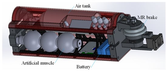
Figure 5.
3DCAD model of the developed Joint Module.
4. Basic Properties
4.1. Elastic Element Evaluation Experiment
The elastic elements of the Joint Module are evaluated in this section. The tracking performance of the joint angle, joint stiffness, and output torque to the command value are all evaluated in this experiment. In contrast, this experiment has a sampling period of 0.001 s.
4.1.1. Experimental Environment
The experimental environment for the elastic element evaluation experiment is depicted in Figure 6. A personal computer sends commands to the developed Joint Module, which is mounted on the base in the direction that the driving arm drives horizontally. Sensors mounted on the Joint Module measure the joint angle and the pressure applied to the artificial muscles. The torque is calculated by pushing back an aluminum rod (length: 787 mm, mass: 0.46 kg) attached to the end of the Joint Module to a specified angle and multiplying the reaction force by the radius of rotation.
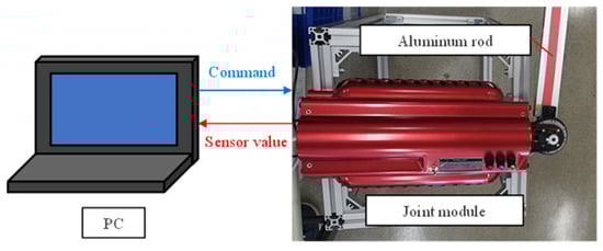
Figure 6.
Diagram of the experimental environment for elastic element experiment.
4.1.2. Joint Angle Measurement Experiment
The joint angle command value is given to the Joint Module every 10 deg in the range of 0 to 180 deg in the joint angle measurement experiment, and the angle read by the encoder is compared with the commanded angle. The number of experiments was set to three, the commanded joint stiffness was set to 0.050 Nm/deg, and the applied pressure was set to 0.30 MPa. Figure 7 shows the vertical axis representing the measured angle, the horizontal axis representing the commanded angle, the points on the graph representing the average of the measured joint angles, and the solid line on the graph representing the target value. In this experiment, the maximum standard deviation was 2.41 deg, so the reproducibility of the joint angle control is high. Figure 7 shows that the measured angle values have hysteresis. This is due to the hysteresis in the contraction characteristics of the artificial muscle. Furthermore, the measured angle deviates from the ideal value by up to 10.5% from the maximum range of motion. We believe this is because the artificial muscles were unable to contract as much as they should have due to the basal friction of the MR brake connected to the driveshaft.
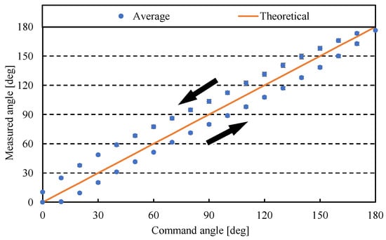
Figure 7.
Measurement results of joint angles. In this graph, the vertical axis represents the measured angle, and the horizontal axis represents the target angle.
4.1.3. Joint Stiffness Measurement Experiment
The command angle is fixed at 90 deg in the joint stiffness measurement experiment, and the commanded joint stiffness is increased from 0.04 Nm/deg to 0.12 Nm/deg in steps of 0.02 Nm/deg until the pressure limit is reached, and each joint stiffness is measured six times. The experiment has a pressure limit of 0.30 MPa. First, measure the reaction force by pushing the arm at an arbitrary angle from the command angle. At this point, the arm motion angle was adjusted by 10 deg from −30 to +30 deg, and the measurement was taken at each motion angle. The measured reaction force was converted to a torque, which was calculated by dividing the torque by the arm’s movement angle. Figure 8 depicts the results of this experiment, with the vertical axis representing the measured joint stiffness, the horizontal axis representing the commanded joint stiffness, the points on the graph representing the actual measured joint stiffness, and the solid line on the graph representing the target value. Figure 8 depicts how the magnitude of the joint stiffness varies with the commanded joint stiffness value. This implies that the Joint Module has variable stiffness properties. However, the value of the joint stiffness varies depending on the arm’s movement angle. Furthermore, the joint stiffness value deviates greatly from the command value. We believe that this is because of the nonlinearity of artificial muscle contraction force characteristics.
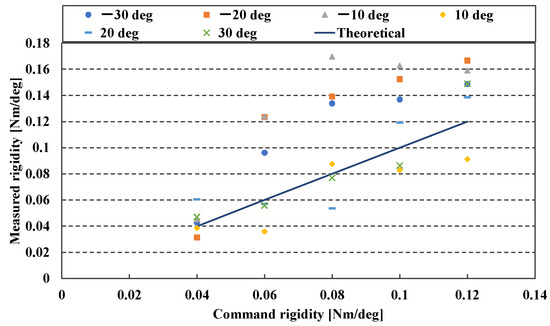
Figure 8.
Results of additional experiments on joint stiffness measurement. In this graph, the vertical axis represents the measuring joint stiffness, and the horizontal axis represents the target joint stiffness.
4.1.4. Output Torque Measurement Experiment
An arbitrary joint angle is used as a command value in the output torque measurement experiment. Then, the command value of the output torque is varied by 1 Nm in the range of −3 to +3 Nm at each joint angle. At this point, the reaction force is measured, and the output torque is calculated. However, for the sake of simplicity, this experiment was carried out with the commanded joint stiffness set to 0.05 Nm/deg. The measurement results of the output torque are shown in Figure 9. In Figure 9, the vertical axis is the output torque, the horizontal axis is the joint angle, the dashed lines on the graph represent the target output torques, and the points on the graph represent the measured output torques. Figure 9 depicts how the output torque varies with the command value. As a result, we believe that the output torque of the Joint Module can be controlled. However, the value of the output torque varies depending on the joint angle. This is because of the nonlinearity of the artificial muscles’ contraction force characteristics.
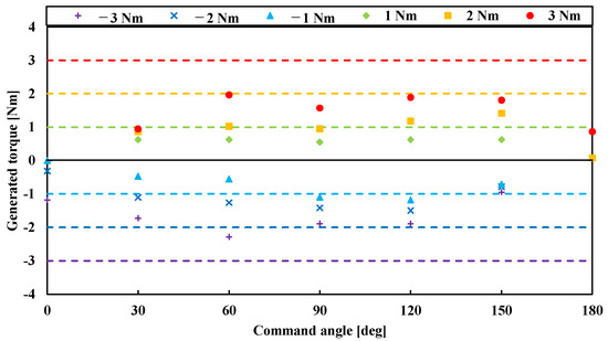
Figure 9.
Measurement results of generated torque. In this graph, the vertical axis represents the generated torque, and the horizontal axis represents the command angle.
4.2. Viscous Element Evaluation Experiment
In this section, we experiment to assess the viscous element of the Joint Module. The viscous element is linked to the MR brake, and the apparent viscosity is achieved by adjusting the MR brake’s frictional torque with the drive arm’s angular velocity. In the experiments of this section, we evaluate the tracking performance of the MR brake about the commanded viscosity when it is controlled according to the angular velocity. However, the sampling period in this experiment was set to 0.001 s.
4.2.1. Experimental Environment
The experimental environment for the viscous element evaluation experiment is depicted in Figure 10. The Joint Module is attached to the base in the direction that the drive arm drives vertically in this experiment, and an aluminum rod (length 398 mm, mass 0.061 kg) and a weight (mass 0.81 kg) are attached to the drive arm of the Joint Module. The joint modules viscosity command ranges from 0.04 and 0.10 Nm s/deg. When the weight is allowed to fall freely at each command value, the joint angle and angular velocity are measured. The torque balance at the center of rotation is used to calculate joint viscosity based on the measured values.
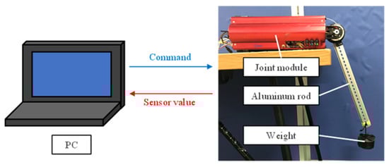
Figure 10.
Diagram of the experimental environment for viscous element experiment.
4.2.2. Experimental Results
The experimental results are depicted in Figure 11. In Figure 11, the vertical axis is the measured torque, the horizontal axis is the joint angular velocity, the solid line on the graph is the actual measured value, and the dotted line is the approximate line of the measured value obtained by the least-squares method. The slope in Figure 11 represents the joint viscosity. Figure 11 depicts how the viscosity value changes in response to changes in the viscosity command value. This means that the Joint Module has a variable viscosity property. The graph also shows hysteresis, which is thought to be a hysteresis curve due to the effect of the residual magnetic field generated when a magnetic field is applied to the MR brake. When the angular velocity is 0 deg/s, the measurement’s endpoint is not at the origin, and the load torque exists. This is because the weight came to a halt in the middle of its descent. Based on this result, we can conclude that the MR brakes viscosity control suppresses the weight’s inertia when it falls. Next, we compare the commanded viscosity and the slope of the approximate line in Table 2. Table 2 shows that for all the viscosities tested in this research, the error between the commanded and measured values is less than 7%. For all viscosities tested in this research, the error between the command value and the measured value is less than 7%. As a result, we believe that following up on the viscosity elements to the specified value is sufficient.
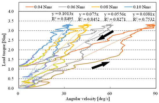
Figure 11.
Measurement results of joint viscosity.
Table 2.
The measured value for joint viscosity command value.
5. Characterization of a Variable Viscoelastic Joint Module
In this chapter, we use experiments to assess the change in motion and response to disturbance of the Joint Module caused by the driving method. However, the sampling period in this experiment is 0.001 s.
5.1. Change in Motion by the Driving Method
5.1.1. Experimental Environment
The experimental environment for assessing motion change using the drive method is essentially the same as described in Section 4.1.1. However, nothing is attached to the drive arm of the Joint Module in this experiment, and the joint angle is measured using the encoder in the Joint Module. The command value of the joint angle of the Joint Module is changed from 0 to 90 deg and the command value of the joint angle of the Joint Module is changed from 0 to 90 deg. The joint angles were calculated by comparing motions of instantaneous motion with the MR brake, varying the viscous command, applying constant friction with the MR brake, and driving without the MR brake. However, the number of trials in this experiment was limited to five, and the commanded value of joint stiffness was set to 0.050 Nm/deg. The following section explains the specific driving method for instantaneous motion.
5.1.2. Driving Method for Instantaneous Motion
Figure 12 depicts a high-level overview of the instantaneous motion drive method. The procedure below is used to drive the instantaneous motion.
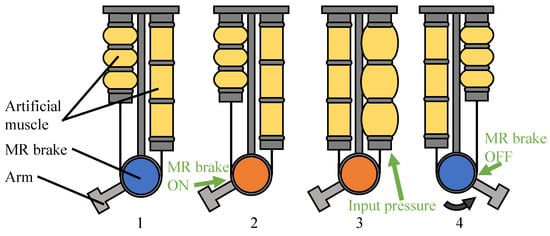
Figure 12.
Schematic diagram of instantaneous operation.
- Set the joint angle command to the initial angle and adjust the drive arm position to the initial angle.
- Turn on the MR brake to prevent the drive arm from moving.
- Send the angle command of the target angle while the MR brake is turned on.
- Release the MR brake to move quickly to the target angle (generation of instantaneous motion).
5.1.3. Experimental Results
Figure 13 depicts the results of the experiment without MR brake and with instantaneous motion. In Figure 13, the horizontal axis represents measurement time, while the vertical axes represent (a) angle and (b) angular velocity, respectively. The blue line represents the average value of the measurement data without the use of an MR brake, and the orange line represents the average value of the measurement data with instantaneous motion. The wasted time element is reduced by the instantaneous motion, as depicted in Figure 13a. There is a time lag between the pressure command and the actual contraction because the artificial muscle is pneumatically driven. The time lag characteristics of artificial muscles were reduced by accumulating the potential in advance using the MR brake when using the instantaneous motion method. Figure 13b shows that the angular velocity is larger when the instantaneous motion is performed than when the MR brake is not used. Based on the this, we can conclude that the instantaneous motion is useful when quick movement is required or when we want to reduce the time lag.
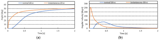
Figure 13.
Measurement results of instantaneous drive and normal drive. (a) Results of angle. (b) Results of angular velocity.
Next, Figure 14 depicts the experimental results when the viscosity command is varied. The horizontal axis in Figure 14 represents measurement time, while the vertical axes represent (a) angle and (b) angular velocity, respectively. The blue line represents the average of the measured data when the MR brake is turned off, the orange line represents the commanded viscosity of 0.020 Nm s/deg, the gray line represents the commanded viscosity of 0.040 Nm s/deg, and the yellow line represents the commanded viscosity of 0.060 Nm s/deg. The gray and yellow lines are the average values of the measured data when the viscosity is 0.020 Nm s/deg, 0.040 Nm s/deg, and 0.060 Nm s/deg, respectively. Figure 14a shows that as the viscosity command value increases, the angle rises more gradually. Figure 14a shows that the rise of the angle becomes slower as the viscosity command increases, and Figure 14b shows that the angular velocity is suppressed as the viscosity command increases. According to the preceding, controlling the joint viscosity can control the angular velocity without fine-tuning the applied pressure to the artificial muscle or the flow rate of the applied air. As a result, the drive with the viscosity command is appropriate for controlling the angular velocity.
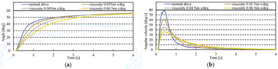
Figure 14.
Measurement results of viscous drive and normal drive. (a) Results of angle. (b) Results of angular velocity.
Finally, Figure 15 depicts the experimental results of driving with constant friction applied by the MR brake. In Figure 15, the horizontal axis represents the measurement time, and the vertical axes represent (a) angle and (b) angular velocity, respectively. The blue line represents the average of the measured data without the use of an MR brake, the orange line represents the commanded friction torque of 1.0 Nm, the gray line represents the commanded friction torque of 1.5 Nm, and the yellow line represents the commanded friction torque of 2.0 Nm. Figure 15 shows the average of the measured data. Figure 15a shows that the dead time increases as the friction torque increases. In addition, the final obtained angle decreases. We believe this is because the force required for the artificial muscle to contract increases as the friction torque increases. The increase in friction torque increased the supply pressure required for the artificial muscle to begin contracting, and because the artificial muscle contraction force is proportional to the amount of contraction, the artificial muscle could not contract before reaching the target angle. As the frictional torque increases, the angular velocity dead time increases and the peak value decreases, as shown in Figure 15b. Because changing the viscous command can reduce the peak value of the angular velocity, it is more effective to use the constant friction as a brake during the motion.
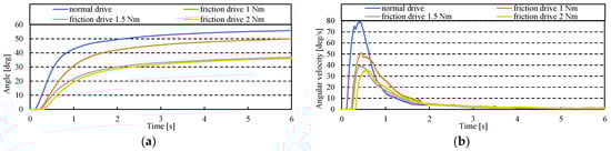
Figure 15.
Measurement results of friction drive and normal drive. (a) Results of angle. (b) Results of angular velocity.
5.2. Response to Disturbance
5.2.1. Modeling of Disturbance Response
The angular response was confirmed by simulation in the disturbance response experiment to be conducted this time. The mechanical model of the experimental environment used in this research is depicted in Figure 16, and the parameters used in this model are depicted in Table 3. This is a mechanical model of a rotating system with a spring, mass, and damper. In the actual experiment, the spring represents the artificial muscle, the mass represents the moment of inertia of the Joint Module and the drive arm, and the damper represents the MR brake. The MR brakes viscosity, on the other hand, is represented by the base viscosity and the viscosity under control. Equation (11) is used to calculate the viscosity due to control, assuming that the torque response of the MR brake is a first-order delay system. The simulation was carried out using computational software (Simulink, Math Works).
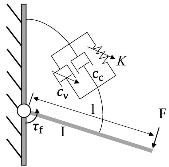
Figure 16.
Simulation model of disturbance response experiment.
Table 3.
Parameters used in the simulation of the characterization experiment.
Three experiments were carried out in this experiment: static load, load removal, and crash. In the static loading experiment, we looked at how a Joint Module with an arbitrary angular command behaves when a static load is applied. In the load-removal experiment, we look at how the behavior changes depending on the command value when a load is removed from a Joint Module that has a static load applied to it by giving an arbitrary angle command. The collision experiment investigates the behavior change based on the command value when an impact force is applied to the Joint Module with an arbitrary angle command. A rising step input was used in the simulation for the static load experiment, a falling step input for the load removal experiment, and an impulse input was used for the collision experiment.
5.2.2. Static Load Experiment
When a static load is applied to a Joint Module with an arbitrary angle command, the change in behavior with command value was investigated experimentally in the static loading experiment. In this experiment, we measured the response of the driving arm of the Joint Module when a static load is applied. The experimental environment for the static load experiment is depicted in Figure 17a,b. The Joint Module is mounted on the base in the direction that the drive arm is driven vertically in this experiment, and an aluminum rod (300 mm long, 0.11 kg mass) is attached to the drive arm of the Joint Module. A weight (0.81 kg in mass) is carefully placed on the end of an aluminum rod with the command angle set to 90 deg, resulting in an initial velocity becoming 0 m/s. The stiffness and viscosity of the joint are measured. The encoder mounted on the Joint Module measures the response when the command values of the joint stiffness and joint viscosity are changed. The number of trials in this experiment was set to five, and all experimental data were averaged.
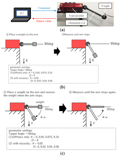
Figure 17.
Diagram of the experimental environment for static load and load removal experiment. (a). Actual experimental environment diagram. (b). Flowchart of experimental environment for static load experiment. (c). Flowchart of experimental environment for load removal experiment.
The simulation and experimental results of this experiment are depicted in Figure 18. In Figure 18, the dashed line shows the simulation result, and the solid line shows the experimental result. (a) shows the result for varying the joint stiffness, and (b) shows the result of varying the joint viscosity. In Figure 18a, the horizontal axis is the measurement time, and the vertical axis is the changing angle. When the stiffness command is 0.050 Nm/deg, the blue line is the average value of the measured data, the orange line is 0.075 Nm/deg, and the gray line is 0.10 Nm/deg. The simulation result in Figure 18a shows that the angle change tends to become smaller as the stiffness command value increases. Following that, the experimental result shows that as the joint stiffness command value increases, the displacement angle decreases This trend we believe, corresponds to the simulation result. This is because the applied pressure to the artificial muscle increases as the stiffness command increases, and the torque required to change the joint angle increases as the stiffness command increases. Based on the this, the Joint Module can deform in response to external forces, and the degree of deformation can be adjusted by changing the command stiffness. As a result, by varying the command stiffness based on the operating environment, the joint can respond to various environments.
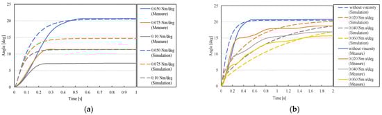
Figure 18.
Simulation and measurement results of static load experiment. (a) Result of angle (joint stiffness). (b) Result of angle (joint viscosity).
Figure 18b depicts the experimental result when the joint viscosity was varied. This experiment was carried out with the stiffness command value set to 0.050 Nm/deg. In Figure 18b the horizontal axis represents the measurement time, and the vertical axis represents the changing angle. The blue line represents the average value of the measured data when no viscosity command is present, the orange line represents the viscosity command 0.020 Nm s/deg, the gray line represents the viscosity command 0.040 Nm s/deg, and the yellow line represents the viscosity command 0.060 Nm s/deg. According to the simulation result in Figure 18b, as the viscosity command value increases, the angle change becomes more gradual, and the final angle change becomes smaller. Following that, the experimental result shows that as the joint viscosity increases, the angle change becomes more gradual, and the final angle change also decreases. This we believe, is the same trend as the simulation result. This implies that changing the viscosity command can reduce the peak value of the disturbance.
5.2.3. Load Removal Experiment
The load-removal experiment investigates the change in behavior depending on the command value when the load is removed from a Joint Module with a static load applied by giving an arbitrary angle command. We measured the response in this experiment when the load applied to the joint modules drive arm is abruptly removed. The load removal experiment takes place in the same experimental environment as the static load experiment (Figure 17a,c). In this experiment, the Joint Module was mounted on the base with the drive arm vertically driven, and an aluminum rod (300 mm in length, 0.11 kg in mass) was attached to the drive arm of the Joint Module. A weight (0.81 kg in mass) was attached to the end of an aluminum rod with the command angle set to 90 deg, and the weight was removed by pulling the string attached to the weight. When the command values changed, the encoder mounted on the Joint Module measured the response of the joint stiffness and viscosity. In this experiment, the number of trials was set to five, and all experimental data were averaged.
The simulation and experimental results of this experiment are depicted in Figure 19. In Figure 19, the dashed line shows the simulation result, and the solid line shows the experimental result, and the result for varying the joint stiffness is shown in (a), and for varying the joint viscosity in (b). In Figure 19a, the horizontal axis is the measurement time, and the vertical axis is the changing angle. The blue line represents the average value of the measured data when the stiffness command is set to 0.050 Nm/deg, the orange line is set to 0.075 Nm/deg, and the gray line is set to 0.10 Nm/deg. To begin, the simulation result in Figure 19a shows that as the stiffness command value increases, the angle change decreases. The displacement angle decreases as the joint stiffness command value increases, according to experimental results This follows the same pattern as the simulation result. According to the preceding, changing the joint stiffness can alter the effects of vibration and angle change caused by external disturbance.
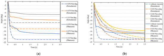
Figure 19.
Simulation and measurement results of load removal experiment. (a) Result of angle (joint stiffness). (b) Result of angle (joint viscosity).
Figure 19b depicts the experimental result when the joint viscosity was varied. This experiment was carried out with the stiffness command value of 0.050 Nm/deg. In Figure 19b, the horizontal axis is the measurement time, and the vertical axis is the angle change, respectively. The blue line represents the mean value of the measured data when no viscosity command is applied, the orange line represents the viscosity command of 0.020 Nm s/deg, the gray line represents the viscosity command of 0.040 Nm s/deg, and the yellow line represents the viscosity command of 0.060 Nm s/deg. When the viscosity is 0.060 Nm s/deg, the yellow line represents the average of the measured data. The simulation results show that as the viscosity command value increases, the angle change becomes more gradual, with a smaller final angle change. Following that, as the joint viscosity increases, the angle change becomes more gradual, and the final angle change decreases. This we believe, is the same trend as the simulation result. This suggests that by changing the viscosity command, the effect of disturbance can be mitigated.
5.2.4. Impact Force Experiment
We investigated the change in behavior of a Joint Module with an arbitrary angle command depending on the command value when an impact force is applied to it in the impact force experiment. We measured the response of the joint modules driving arm when it collides with an object in this experiment. The experimental environment for the impact force experiment is depicted in Figure 20a,b. In this experiment, the Joint Module was mounted on a foundation with its driving arm pointing horizontally, and an aluminum rod (length: 300 mm, mass: 0.11 kg) was attached to the driving arm of the Joint Module. A weight (0.81 kg in mass) was hung from the top of the base with a string wrapped around it. The Joint Module was set to 90 deg in this state. The weight was lifted until the string attached to it is parallel to the ground, at which point the hand is released and the weight is struck against the tip of the aluminum rod. The encoder mounted on the Joint Module measures the response of the joint stiffness and the viscosity. The number of trials was set to five, and all experimental data were averaged.
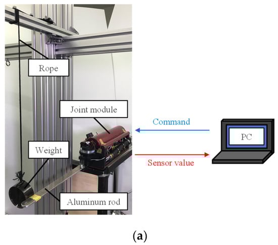
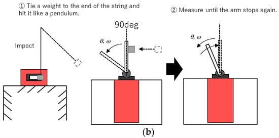
Figure 20.
Diagram of the experimental environment for impact force experiment. (a). Actual experimental environment diagram. (b). Flowchart of experimental environment for impact force experiment.
The simulation and experimental results of this experiment are depicted in Figure 21. In Figure 21, the dashed line shows the simulation results, and the solid line shows the experimental results. The results of varying the joint stiffness are shown in (a), and the results of varying the joint viscosity are shown in (b). The horizontal axis in Figure 21 (represents the measurement time, the vertical axis represents the angle, and the blue line represents the average value of the measured data when no command was given to the device, the orange line represents the stiffness command of 0.050 Nm/deg, the gray line represents the stiffness command of 0.075 Nm/deg, and the yellow line represents the stiffness command of 0.10 Nm/deg. First, the simulation results show that when the stiffness command is issued, the angle returns to its initial value. The tendency to return to the initial angle becomes stronger as the stiffness command value increases, following that, the experimental results revealed that when the stiffness command was issued, the motion returned to its initial angle, confirming the same trend as the simulation results. When the stiffness command was increased, the peak of the angle change shrank. In contrast, the peak value of the angle change was greater for 0.10 Nm/deg than for 0.075 Nm/deg of the stiffness command.
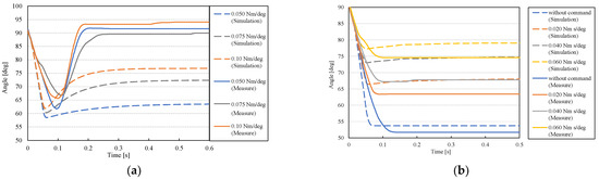
Figure 21.
Simulation and measurement results of impact force experiment. (a) Results of angle (joint stiffness). (b) Results of angle (joint viscosity).
This experiment was conducted without the use of a stiffness command value. The horizontal axis in Figure 21b is the measurement time and the vertical axis is the angle. The blue line represents the average value of the measured data when no viscosity command is present, the orange line represents the viscosity command of 0.020 Nm s/deg, the gray line represents the viscosity command of 0.040 Nm s/deg, and the yellow line represents the viscosity command of 0.060 Nm s/deg. The simulation results show that as the viscosity command value increases, the angle change decreases and as the joint viscosity increases, the change in angle is gradual and small, according to the experimental results. This is the same trend as shown by the dashed line in the simulation. This suggests that increasing the viscosity command can quickly dampen the disturbance caused by the impact force.
Finally, when the stiffness and viscosity commands were given simultaneously, a disturbance response experiment to the impact force was performed. This time, we’ll look at a stiffness command of 0.075 Nm/deg and a viscosity command of 0.040 Nm s/deg are given as representative values. Figure 22 depicts the simulation and experimental results of this experiment. In Figure 22, the horizontal axis represents the measurement time and the vertical axis represents the angle, and the blue line represents the time when no command is given, the orange line represents the time when only the stiffness command of 0.075 Nm/deg is given, the gray line represents the time when only the viscosity command of 0.040 Nm s/deg is given, and the yellow line represents the time when the stiffness command of 0.075 Nm/deg and the viscosity command of 0.040 Nm s/deg are given simultaneously. The average value of the measured data is represented by the entire line. Figure 22 shows that when the stiffness and viscosity commands are given simultaneously, the peak of the angle change is suppressed the most, but the final angle does not return to the initial angle. When the stiffness and viscosity commands are given simultaneously, the peak of the disturbance is suppressed the most.
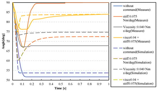
Figure 22.
Simulation and measurement angle of impact force experiment results of angle.
6. Comparison with Existing Modular Robots
We compared the Joint Module to existing modular robots [13,14,15,16,17]. In this section. Modular robots’ basic components are mass, size, output power, range of motion, and inertia. In this research, we focused on the device’s output power and inertia and compared them using an index (output power-inertia ratio) calculated by dividing the maximum output power Pmax by the rotor inertia moment Ir. The greater the value of this index, the lower the inertia and the higher the output power of the device. Table 4 depicts a comparison table between the Joint Module and existing modular robots. Table 4 shows that the output power-to-inertia ratio is more than 10 times higher than that of other modular robots. We believe that this is because the Joint Module has a lower moment of inertia than other robots.
Table 4.
Comparison table of a variable viscoelastic Joint Module and existing module.
Table 4.
Comparison table of a variable viscoelastic Joint Module and existing module.
| Comparison Items (Modular Robots with Built-In Control Device) | This Study Joint Module | X5-1 [13] | X5-9 [13] | X8-3 [13] | X8-16 [13] | KM-1U [14] | KM-1S-M4021 [15] | KM-1S-M6829 [15] | qb Move ADVANCED [16] | Mori [17] (Origami Robots) |
|---|---|---|---|---|---|---|---|---|---|---|
| (Pmax/It [×103 W/(kg·m2)] | 61.0 | 5.38 | 0.131 | 5.61 | 0.195 | - | - | - | - | - |
| Maximum power Pmax [W] | 18.3 | 17.1 | 17.1 | 35.4 | 35.4 | 2.04 | 1.87 | 1.81 | 38.5 | - |
| Morment of inertial It [×10−3 (kg·m2)] | 0.300 | 3.19 | 130 | 6.30 | 182 | - | - | - | - | 0.0472 |
| Mass (without power source) [kg] | 2.61 | 0.330 | 0.360 | 0.455 | 0.496 | 0.340 | 0.0690 | 0.195 | 0.450 | 0.0260 |
| Volume [×10−3 m3)] | 10.2 | 0.249 | 0.249 | 0.361 | 0.361 | 0.166 | 0.101 | 0.194 | 0.314 | 0.0166 |
| Range of motion [deg] | 90-180 | 360 | 360 | 360 | 360 | 360 | 360 | 360 | ±180 | - |
| Maximum torque [Nm] | 5 | 2.5 | 13 | 7 | 38 | 0.3 | 0.1 | 0.5 | 6.8 | 0.03 |
| Gear ratio | 1 | 272.222 | 1742 | 272.222 | 1462.222 | - | - | - | - | 256 |
| Maximum angular velocity [deg/s] | 457 | 540 | 84 | 504 | 90 | 1560 | 4320 | 840 | 363 | 12 |
In terms of maximum torque, the existing module X8-16 [13] has the most. In contrast, the maximum torque can be adjusted by the onboard reduction gear, and without the reduction gear, the torque generated by the Joint Module is the highest. As a result, this Joint Module has a high torque-to-inertia ratio and can be described as having low inertia and high output torque.
The volume of the Joint Module is the largest. Because the volume of the artificial muscles and pneumatic source used as actuators is large, the Joint Module has the highest volume The Joint Module is the largest in terms of volume. In particular, because the displacement of the artificial muscles is calculated by dividing the contraction rate by length, the size of the artificial muscles must be large enough to account for the large deformation that occurs when they are driven.
Even when the drive source is excluded, the proposed Joint Module has the highest mass when compared to other modules. This is because, unlike the rotating system of a motor, the Joint Module generates tension when the artificial muscle is driven. When 0.3 MPa is applied, the artificial muscle can generate a maximum tension of over 1000 N in the axial direction [18]. Because the Joint Module must have a structure that will not be destroyed by this tension it is considered heavy. However, we believe that by reviewing the materials used in the module we can reduce weight.
The joint modules drive unit cannot rotate indefinitely. This is due to a limitation in the amount of contraction of the artificial muscles. The drive range can be changed by reducing the y diameter of the pulley. In contrast, the torque decreases in inverse proportion to the pulley diameter.
7. Proposed Applications
7.1. Hypothesis for Joint Module Application
Based on the evaluation experiments in Section 4 and Section 5, we discuss suitable devices and environments for the application of the Joint Module in this section. The Joint Module has hysteresis, as determined by the elastic element evaluation experiments in Section 4.1, and there is a difference between the commanded and measured values. As a result, it is unsuitable for precise work such as assembly of parts. Based on the output characteristics evaluated in Section 5.1, the Joint Module can suppress device motion by controlling joint stiffness and joint viscosity. Furthermore, according to the comparison with existing devices in Section 5.2, the rotor moment of inertia is smaller than that of other modular robots. Finally, we believe that the Joint Module is suitable for devices that operate in a human-like environment, such as assistive devices Based on these considerations, we will fabricate a device using the Joint Module in the following section.
7.2. Application Example 1: Training of a Single Joint
Because the training device operates close to the human body, the danger that may occur if the timing of the movement between the device and the person does not match must be considered. As a result, to provide a load to the wearer, the training the device itself must have high back-drivability and power. Based on the this, and the discussion in Chapter 6, we created a human training device for a single joint as one of the applications of the Joint Module. The device is depicted in Figure 23. This device is made up of a Joint Module and has a fixture attached to it. We carried out an experiment wherein we applied a load to the subjects using the device that we built.
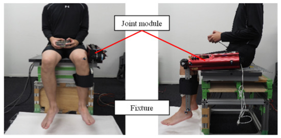
Figure 23.
The appearance of a single joint training device that applies a Joint Module.
One healthy male subject (age: 22 years, height: 175 cm, weight: 55 kg) was asked to perform a leg swinging motion while sitting on a table. At this time, we measured the surface EMG potential of the semimembranosus muscle and compared the number of muscle activities with and without the device, as well as with changes in the command joint angle. When the leg was horizontal to the ground, the angle of the knee joint was set to 0 deg, and the direction of leg extension was set to the positive direction. The “Ethical Review of Research on Human Subjects, Faculty of Science and Engineering, Chuo University” approved the experiments on human subjects described in this paper (Approval No. 2020-25). human, and was designed to be attached to a human lower limb.
Figure 24 depicts the results of this experiment. The vertical axis in Figure 24 represents the surface EMG potential, the horizontal axis represents the motion period, and the black solid line represents the measurement data without the device, the black dashed line represents the command angle of 0 deg, the gray solid line represents the command angle of 45 deg, and the gray dashed line represents the command angle of 90 deg. Figure 24 shows that the device is used, the surface EMG values are higher than when it is not used. Furthermore, the larger the command angle, the greater the surface EMG value. Using the Joint Module, we believe that we have successfully applied a load to a human.
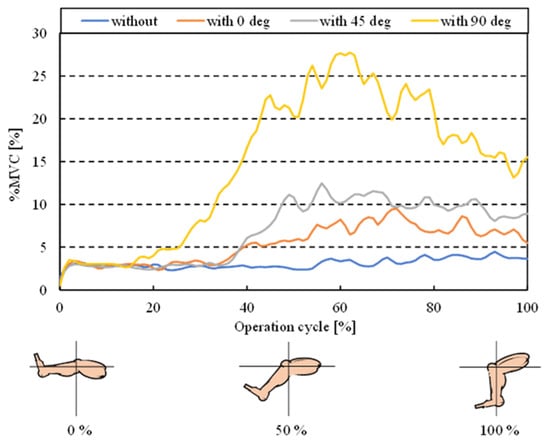
Figure 24.
The result of the training experiment.
7.3. Application Example 2: Four-Segment Parallel Link Mechanism
We used the Joint Module to fabricate a device that drives a four-section parallel link mechanism as one of its applications. Figure 25 depicts the device. The joint modules are arranged back-to-back in this device, the drive axes are arranged on the same axis, and the four-section parallel linkage mechanism is controlled by varying the angles of the two joint modules. We believe that by varying the combinations of the joint modules, this system can be applied to a variety of applications without significantly altering the design.
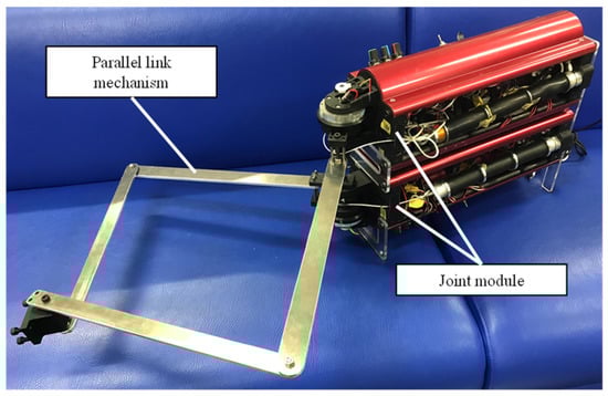
Figure 25.
Picture of application examples of the Joint Module (four-section parallel link mechanism).
8. Conclusions
- The following is a synopsis of the paper’s contents. Based on previous research using variable viscoelastic drive joints that mimic the human joint drive principle, we proposed a variable viscoelastic drive Joint Module.
- A description of the structure of the developed Joint Module is provided. The module, which includes a drive unit, a pneumatic system, a control unit, an electrical system, sensors, and an interface, can be driven without the use of an external system.
- We evaluated the basic characteristics of the developed Joint Module. As the basic characteristics, the tracking performance of the joint angle, joint stiffness, generated torque, and joint viscosity to the command value was confirmed by experiments.
- The developed Joint Module was used to assess the properties of a variable viscoelastic drive joint. To evaluate the characteristics, the change in motion and the response to the external disturbance caused by the difference in driving methods were confirmed by simulation and experiment.
- We discussed what kind of device the Joint Module is suitable for based on the results of the basic characteristics evaluation and the characteristics evaluation of the variable viscoelastic drive joint. Based on the findings, two types of applications of the Joint Module were proposed.
Based on these findings, we conclude that the Joint Module is suitable for operation in a human-like environment.
We will investigate the possibility of expanding the operating environment in the future by modularizing the variable viscoelastic drive joints for use in environments other than the laboratory. When the joint module’s mass and volume were compared to those of existing modules, it was discovered that the mass and volume of the joint module were greater than those of other existing modules. Based on these findings, we will create a smaller and lighter Joint Module.
Author Contributions
Conceptualization, T.F., K.M., T.N. and M.O.; methodology, T.F.; software, M.O.; validation, T.F., R.N., Y.S. and K.M.; formal analysis, T.F.; investigation, T.F.; resources, T.F. and M.O.; data curation, T.F.; writing—original draft preparation, T.F.; writing—review and editing, M.O., R.N. and T.N.; visualization, T.F.; supervision, T.N.; project administration, T.N.; funding acquisition, T.N. All authors have read and agreed to the published version of the manuscript.
Funding
This study was supported by the New Energy and Industrial Technology Development Organization (NEDO).
Institutional Review Board Statement
This study was approved by the Ethical Review for Research Involving Human Subjects, Faculty of Science and Engineering, Chuo University (No. 2020-25).
Informed Consent Statement
The purpose and methods of the experiment were explained to all subjects involved in this experiment, and their consent to participate in the experiment was obtained.
Conflicts of Interest
The authors declare no conflict of interest. The funders had no role in the design of the study; in the collection, analyses, or interpretation of data; in the writing of the manuscript, or in the decision to publish the results.
References
- YASKAWA. Available online: https://www.yaskawa.co.jp/product/robotics (accessed on 5 January 2020).
- CYBERDYNE. Available online: https://www.cyberdyne.jp/products/HAL/index.html (accessed on 14 November 2019).
- SoftBank. Available online: https://www.softbank.jp/robot/pepper/ (accessed on 14 November 2019).
- Okui, M.; Iikawa, S.; Yamada, Y.; Nakamura, T. Fundamental characteristic of novel actuation system with variable viscoelastic joints and magneto-rheological clutches for human assistance. J. Intell. Mater. Syst. Struct. 2018, 1, 82–90. [Google Scholar] [CrossRef] [Green Version]
- Versaci, M.; Cutrupi, A.; Palumbo, A. A Magneto-Thermo-Static Study of a Magneto-Rheological Fluid Damper: A Finite Element Analysis. IEEE Trans. Magn. 2021, 57, 1–10. [Google Scholar] [CrossRef]
- Nagayama, T.; Ishihira, H.; Tomori, H.; Nakamura, T. Verification of throwing operation by a manipulator with variable viscoelastic joints with straight-fiber-type artificial muscles and magnetorheological brakes. Adv. Robot. 2016, 30, 1365–1379. [Google Scholar] [CrossRef]
- Okui, M.; Iikawa, S.; Yamada, Y.; Nakamura, T. Variable Viscoelastic Joint System and Its Application to Exoskeleton. In Proceedings of the IEEE/RSJ International Conference on Intelligent Robots and Systems (IROS), Vancouver, BC, Canada, 24–28 September 2017. [Google Scholar]
- Ministry of Economy, Trade and Industry. Market Trend of Robot Industry. 2012. Available online: https://www.meti.go.jp/policy/mono_info_service/mono/robot/pdf/20130718002-3.pdf (accessed on 23 February 2021).
- Machida, K.; Kimura, S.; Suzuki, R.; Yokoyama, K.; Okui, M.; Nakamura, T. Variable Viscoelastic Joint Module with Built-in Pneumatic Power Source. In Proceedings of the 2020 IEEE/ASME International Conference on Advanced Intelligent Mechatronics (AIM), Boston, MA, USA, 6–9 July 2020; pp. 1048–1055. [Google Scholar]
- Baca, J.; Ferre, M.; Campos, A.; Fernandez, J.; Aracil, R. On the Analysis of a Multi-Task Modular Robot System for Field Robotics. In Proceedings of the IEEE Electronics, Robotics and Automotive Mechanics Conference, Cuernavaca, Mexico, 28 September–1 October 2010. [Google Scholar]
- Guan, Y.; Jiang, L.; Zhang, X.; Qiu, J.; Zhou, X. 1-DoF Robotic Joint Modules and Their Applications in New Robotic Systems. In Proceedings of the 2008 IEEE International Conference on Robotics and Biomimetics, Bangkok, Thailand, 21–26 February 2006; p. 1905. [Google Scholar]
- Suzuki, R.; Okui, M.; Iikawa, S.; Yamada, Y.; Nakamura, T. Novel Feedforword Controller for Straight-Fiber-Type Artificial Muscle Based on an Experimental Identification Model. In Proceedings of the 2018 IEEE International Conference on Soft Robotics (RoboSoft), Livorno, Italy, 24–28 April 2018; pp. 31–38. [Google Scholar]
- Okui, M.; Nagura, Y.; Yamada, Y.; Nakamura, T. Hybrid Pneumatic Source Based on Evaluation of Air Compression Methods for Portability. IEEE Robot. Autom. Lett. 2018, 3, 819–826. [Google Scholar] [CrossRef]
- HEBI Robotics. Available online: https://docs.hebi.us/hardware.html#x-series-actuators (accessed on 3 November 2021).
- Keigan Motor. Available online: https://keigan-motor.com/km-1s/ (accessed on 20 January 2022).
- qb Robotics. Available online: https://qbrobotics.com/products/qbmove-advanced/# (accessed on 20 January 2022).
- Belke, C.H.; Paik, J. Mori: A Modular Origami Robot. IEEE/ASME Trans. Mechatron. 2017, 22, 2153–2164. [Google Scholar] [CrossRef]
- Kojima, A.; Okui, M.; Yamada, Y.; Nakamura, T. Prolonging the lifetime of straight-fiber-type pneumatic rubber artificial muscle by shape consideration and material development. In Proceedings of the International Conference on Soft Robotics, Livorno, Italy, 24–28 April 2018. [Google Scholar]
Publisher’s Note: MDPI stays neutral with regard to jurisdictional claims in published maps and institutional affiliations. |
© 2022 by the authors. Licensee MDPI, Basel, Switzerland. This article is an open access article distributed under the terms and conditions of the Creative Commons Attribution (CC BY) license (https://creativecommons.org/licenses/by/4.0/).