Article

Exploiting Cyclic Angle-Dependency in a Kalman Filter-Based Torque Estimation on a Mechatronic Drivetrain

1
Leuven Mechatronic System Dynamics (LMSD), Department of Mechanical Engineering, KU Leuven, 3000 Leuven, Belgium
2
DMMS Core Lab, Flanders Make, 3001 Heverlee, Belgium
3
MotionS Core Lab, Flanders Make, 3001 Heverlee, Belgium
*
Author to whom correspondence should be addressed.
Actuators 2022, 11(2), 35; https://doi.org/10.3390/act11020035
Submission received: 24 December 2021 / Revised: 17 January 2022 / Accepted: 20 January 2022 / Published: 24 January 2022
(This article belongs to the Special Issue Design of Sensing and Actuation Systems)

Abstract

:
Torsional vibrations play a critical role in the design and operation of a mechanical or mechatronic drivetrain due to their impact on lifetime, performance, and cost. A magnetic spring allows one to reduce these vibrations and improve the actuator performance yet introduces additional challenges on the identification. As a direct torque measurement is generally not favourable because of its intrusive nature, this paper proposes a nonintrusive approach to identify torsional load profiles. The approach combines a physics-based lumped parameter model of the torsional dynamics of the drivetrain with measurements coming from a motor encoder and two MEMS accelerometers in a combined state/input estimation, using an augmented extended Kalman filter (A-EKF). In order to allow a generic magnetic spring torque estimation, a random walk input model is used, where additionally the angle-dependent behaviour is exploited by constructing an angle-dependent estimate and variance map. Experimental validation leads to a significant reduction in bias in the load torque estimation for this approach, compared to conventional estimators. Moreover, this newly proposed approach significantly reduces the variance on the estimated states by exploiting the angle dependency. The proposed approach provides knowledge of the torsional vibrations in a nonintrusive way, without the need for an extensive magnetic spring torque identification. Further, the approach is applicable on any drivetrain with angle-dependent input torques.

1. Introduction

In mechanical and mechatronic drivetrains, torsional loading and vibrations have a critical impact on the lifetime, performance, and cost. For most applications, an assessment of these vibrations requires knowledge of both the system states and the applied torques. Unfortunately, the direct measurement of these variables is infeasible in many applications. This holds especially true for the direct measurement of the applied torques. Possible reasons for this are the high costs and the intrusive nature of torque sensors.
A possible solution is to estimate the unknown torques indirectly from a limited set of measurements. In order to allow such estimation, additional information can be provided by a model of the considered drivetrain. In the literature, several approaches are described to estimate unknown input loads for mechanical systems. Either frequency domain or time domain approaches can be used. The attention has recently been shifting to time domain approaches. Two classes of time domain approaches, namely inverse system methods and Kalman-based techniques, are discussed in the next two paragraphs.
Inverse system methods (summarised by Nordström [1] and Klinkov [2]) use a model of the system to obtain the unknown load from a limited number of response measurements in a deterministic way. As such, these methods assume that an exact model of the system is available. Although a model is logically never exact in practice, these methods prove useful for some structural dynamics applications where a sufficiently high model accuracy can be obtained. Because this is a lot more challenging for drivetrain applications, the deterministic methods are less suitable for those cases.
A more suited alternative is given by Kalman-based estimation techniques, a class of stochastic methods based on the Kalman filter [3,4]. The filter provides an efficient and optimal (with respect to the expected error covariance) solution for the linear state estimation problem. An extension towards nonlinear estimation problems, called the extended Kalman filter (EKF), allows the state estimation of nonlinear systems by linearizing the system matrices around the previous state estimate. More recently, efforts have been made to allow concurrent state, input and parameter estimation. Lourens [5] proposed to augment the states with the unknown forces and to estimate them together in a coupled estimator. Naets [6] elaborated on this idea and presents a generic coupled state/input/parameter estimation framework, by coupling a reduced model to an extended Kalman filter with augmented states for the unknown inputs and parameters.
Applications of these state-augmented Kalman filters on a drivetrain were conducted by Croes [7] and Forrier [8]. In these approaches, a lumped parameter model of the drivetrain is combined with measurements in a state-augmented Kalman filter, where the input torque is included in the estimation as an augmented state. The input is described by a random walk model that uses the previous estimated value as the best guess for the next estimate. This technique allows a generic unknown input estimation but only incorporates little information about the to-be-estimated input. Kirchner [9,10,11] incorporates additional information about the input by mapping it onto a sparsely filled basis within a compressive sensing moving horizon scheme. This method has potential when the input can be described by a set of time-dependent base functions. However, for some applications, there is no time-dependent relationship with respect to the input, but an angle dependency. This is common for linkage mechanisms and cam-drives, applications which are addressed in this work.
More specifically, the considered application consists of a permanent-magnet synchronous motor connected to a crank-rocker mechanism via a torsional magnetic spring. As the magnetic spring torque characteristic is important for the estimation strategy, the background, design, and characteristics of the magnetic spring are briefly described in the next paragraph.
A magnetic spring is a fatigue-free alternative to a mechanical spring, allowing one to improve the energy efficiency of the drivetrain and to downsize the actuator. In order to design such a magnetic spring for a specific application, Mrak [12,13] developed a design methodology and validated this methodology using both virtual designs and one physical prototype. Although this research illustrates the potential benefit of using magnetic springs, it also highlights the complexity of their torque characteristic. Although the static torque characteristic is a quasisinusoidal function of the angle, its exact shape depends on the manufacturing tolerances. Furthermore, the dependency of the magnetic properties on the temperature results in significant stiffness variations with temperature. The dynamic torque additionally has an acceleration-dependent inertia term, speed dependent viscous and eddy current loss terms, and a Coulomb friction loss term.
To allow a generic torque estimation independent of the manufacturing tolerances, the environment, and the drivetrain on which the magnetic spring is mounted, this paper proposes to start from a random walk input model and to detect whether the magnetic spring torque exhibits cyclic angle-dependent behaviour. If this is the case, it exploits this angle-dependent relationship between the magnetic spring torque and the angle in the estimation. This is conducted by constructing and continuously updating an estimation map of the torque and its corresponding variance. By using this map in the estimator, the aim is to reduce the uncertainty of the unknown torque input and consequently improve the estimation.
The lumped-parameter model used in the estimation is described in Section 2. Section 3 discusses the proposed estimation strategy with cyclic periodicity. The experimental validation of this strategy is discussed in Section 4. Section 5 provides a conclusion for the obtained results.

2. Mechatronic Powertrain Model

The mechatronic powertrain is modelled in a MATLAB environment using a lumped-parameter model. Its schematic representation with all relevant variables and parameters is given in Figure 1. The following five subsections describe its submodels: a model of the four-bar linkage, the motor, the magnetic spring, the shaft flexibilities and the torsional losses. The integration of these submodels is described in Section 2.6.

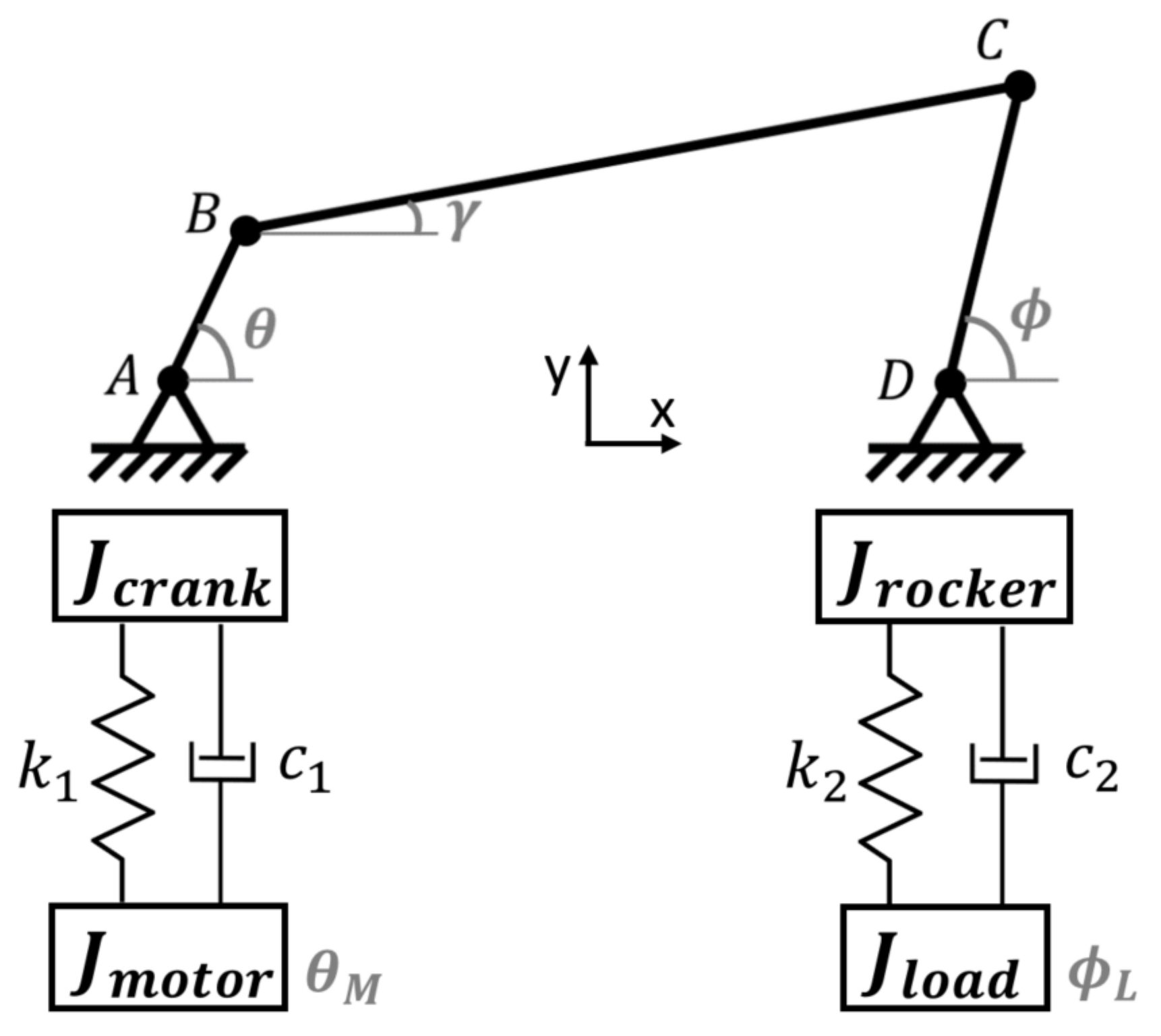
2.1. Four-Bar Linkage Model

The four-bar linkage is categorised as a crank-rocker mechanism according to Grashof’s law [14]. A driving torque on the crank shaft results in a rotating motion of the crank inertia and a reciprocating movement of the rocker inertia. The linkage is modelled as a rigid mechanism. The planar kinematics are described by two loop-closure equations, resulting in a system of two implicit algebraic equations:
a cos θ + h cos γ b cos ϕ g = 0
a sin θ + h sin γ b sin ϕ = 0 ,
where a = | A B | , b = | C D | , h = | B C | , and g = | A D | are the bar lengths measured between two connection points (see Figure 1). The relationship between the velocities can be described by taking the time derivative of Equations (1) and (2):
a θ ˙ sin θ h γ ˙ sin γ + b ϕ ˙ sin ϕ = 0
a θ ˙ cos θ + h γ ˙ cos γ b ϕ ˙ cos ϕ = 0 ,
and correspondingly the accelerations are described by:
a θ ¨ sin θ + h γ ¨ sin γ b ϕ ¨ sin ϕ = a θ ˙ 2 cos θ h γ ˙ 2 cos γ + b ϕ ˙ 2 cos ϕ
a θ ¨ cos θ + h γ ¨ cos γ b ϕ ¨ cos ϕ = a θ ˙ 2 sin θ + h γ ˙ 2 sin γ b ϕ ˙ 2 sin ϕ .
The dynamics are described by the force and moment equilibria, obtained by applying Newton’s second law on the individual members in all directions allowed by the mechanism. The set of equations consists of the moment equilibrium of the crank inertia:
J c r a n k θ ¨ = a F B y cos θ a F B x sin θ + T c r a n k s h a f t ,
the force equilibria (8) and (9) and moment equilibrium (10) of the rod:
m r o d ( a ( θ ¨ sin θ + θ ˙ 2 cos θ ) + 0.5 h ( γ ¨ sin γ + γ ˙ 2 cos γ ) ) = F B x F C x
m r o d ( a ( θ ¨ cos θ θ ˙ 2 sin θ ) + 0.5 h ( γ ¨ cos γ γ ˙ 2 sin γ ) + a g ) = F C y F B y
J r o d γ ¨ = 0.5 h ( cos γ ( F B y + F C y ) sin γ ( F B x + F C x ) ) ,
and the moment equilibrium of the rocker inertia:
J r o c k e r ϕ ¨ = a F B y cos ϕ a F B x sin ϕ + T r o c k e r s h a f t ,
The additional parameters involved in the dynamics are the moment of inertia of the crank ( J c r a n k ), the rod ( J r o d ), the rocker ( J r o c k e r ), and the mass of the rod ( m r o d ). The torques exerted on the crankshaft and rocker shaft are denoted by T c r a n k s h a f t and T r o c k e r s h a f t , respectively. The planar forces at the left and right connection points of the central rod are denoted by ( F B x , F B y ) and ( F C x , F C y ), respectively. a g represents the gravitational acceleration.

2.2. Permanent-Magnet Synchronous Motor Model

The permanent-magnet synchronous motor (PMSM) is modelled as an inertia J m o t o r with a known torque input T m o t o r .

2.3. Magnetic Spring Model

The magnetic spring is connected to the motor shaft, and consequently, its inertia is lumped together in the motor inertia ( J m o t o r ). The spring introduces a torque input T M S on the same inertia.

2.4. Shaft Flexibilities Model

The shaft flexibilities are modelled using a lumped spring-damper model as illustrated on the powertrain model in Figure 1. They introduce two additional degrees of freedom, respectively, the rotation θ M of the drive motor and the rotation ϕ L of the load inertia J l o a d . The flexibilities are parametrised with one torsional stiffness and one torsional damping parameter for each flexible shaft, i.e., ( k 1 , c 1 ) for the motor shaft and ( k 2 , c 2 ) for the load shaft. The torque in the motor shaft and the load shaft is described by the following equations:
T m o t o r s h a f t = k 1 ( θ M θ ) + c 1 ( θ ˙ M θ ˙ )
T l o a d s h a f t = k 2 ( ϕ ϕ L ) + c 2 ( ϕ ˙ ϕ ˙ L )

2.5. Torsional Losses Model

Losses are introduced on each of the three degrees of freedom of the model. The losses consist of simplified frictional and viscous contributions. The frictional loss on the motor inertia T F M is defined as follows:
T F M = T M | θ ˙ M | < θ ˙ 0 & T M T F M , 0 θ ˙ M | θ ˙ M | T F M , 0 otherwise
where T M denotes the resulting torque on the motor inertia without losses, T F M , 0 a friction constant, and θ ˙ 0 the breakaway friction velocity. The viscous losses on the motor inertia T V M are approximated as a linear function of the rotational speed, scaling with c V M :
T V M = c V M θ ˙ M
Analogously, frictional and viscous losses are defined on the load inertia ( T F L , T V L ), the crank inertia ( T F C , T V C ), and the rocker inertia ( T F R , T V R ). As the crank-rocker model is rigid, the crank and rocker shaft rotation describe the same degree of freedom. Due to the difference in speed characteristics, their loss parameters cannot be lumped into one single set.

2.6. Powertrain Model

The complete powertrain model is schematically represented on Figure 1, and it consists of three degrees of freedom: the rotation of the motor inertia, the motion of the four-bar linkage, and the rotation of the load inertia.
The torque on the motor inertia is a combination of the motor drive torque T m o t o r , the torque in the motor shaft T m o t o r s h a f t , the magnetic spring torque T M S , and the loss terms T F M and T V M :
J m o t o r θ ¨ M = T m o t o r T m o t o r s h a f t + T F M + T V M + T M S
The motion of the four-bar linkage is described by Equations (1)–(11). In Equation (7), the term T c r a n k s h a f t sums the motor shaft torque T m o t o r s h a f t and the loss terms T F C and T V C :
T c r a n k s h a f t = T m o t o r s h a f t + T F C + T V C
In Equation (11), the term T r o c k e r s h a f t sums the load shaft torque T l o a d s h a f t and the loss terms T F R and T V R :
T r o c k e r s h a f t = T l o a d s h a f t + T F R + T V R
The torque on the load inertia is a combination of the torque in the load shaft T l o a d s h a f t and the loss terms T F L and T V L :
J l o a d ϕ ¨ L = T l o a d s h a f t + T F L + T V L
This coupled powertrain model is employed in the following sections to perform the estimation on the system under study, with the aim of achieving more insight into the magnetic spring behaviour.

3. Coupled State/Input Estimation with Exploitation of Cyclic Periodicity

For the powertrain described above, the state vector x combines the three rotational degrees of freedom of the model, supplemented with their respective velocities:
x = θ ˙ θ θ ˙ M θ M ϕ ˙ L ϕ L .
The input vector u is given by:
u = T m o t o r T M S
and consists of the torque inputs of the servomotor and the magnetic spring. The continuous-time model equations can be summarised in the following explicit state-space form:
x ˙ = f ( x , u )
where the vector field f describes the equations of motion as discussed in Section 2.
In addition to the model, a set of measurements y is available in the estimator. A motor encoder provides an angle measurement, and two MEMS accelerometers provide triaxial acceleration measurement signals. The accelerometers are mounted on the rocker inertia and on the load inertia with their X-direction aligned with the radial direction of the shaft and their Y-direction with the tangential direction. The axial acceleration signal of the Z-direction is not informative for the torsional dynamics, and it is consequently not used in the estimator. The mapping of the measurement variables on the states and inputs can be written in the following general form:
y = h ( x , u )
where h is a vector of the measurement functions. For the considered case, it consists of five measurement functions. The function for the encoder measurement is trivial and equals the motor angle from the state vector with its corresponding measurement variable. The other four functions describe the acceleration signals of the accelerometers in function of the state vector. Each accelerometer mapping function consists of a static term that describes its direction relative to the gravity vector and a dynamic term that represents either a tangential or a normal acceleration. All terms can be directly calculated when the equations of Section 2 are solved.
The continuous-time equations of the model are time discretised in order to be used in the estimator. The implicit equations are solved iteratively. The model and the measurements are exposed to process and measurement noise, respectively. All noise terms are assumed to be described by zero-mean and uncorrelated normal distributions. The process noise w k and measurement noise v k are quantified with covariance matrices Q and R , respectively. The discrete model and measurement equations are given below:
x k = f d ( x k 1 , u k 1 ) + w k w k N ( 0 , Q ) y k = h ( x k , u k ) + v k v k N ( 0 , R )
where k denotes the iteration step and f d is the time discretisation of f . The applied discretisation procedure is a fourth-order Runge–Kutta integration [15].

3.1. State Augmentation for Magnetic Spring

The magnetic spring described in Section 2.3 generates a torque that is considered as an unknown input to the system. A possible strategy to allow a coupled state/input estimation is augmenting the model states with an unknown input state:
x a u g = x T M S
where T M S denotes the magnetic spring input torque. The corresponding discrete model equations are given as:
f a u g = f d ( x k 1 , u k 1 ) f T M S ( x k 1 , u k 1 )
This strategy requires an additional dynamic model equation for the prediction f T M S ( x k 1 , u k 1 ) of the unknown input. In this work, a random walk (RW) model is adopted:
T M S , k = T M S , k 1 + w R W , k w R W , k N ( 0 , Q R W , k )
where w R W , k denotes the discretisation of a white noise process with zero mean, quantified with a discretised covariance value Q R W , k . The random walk model provides the additional model equation:
f T M S ( x k 1 , u k 1 ) = T M S , k 1

3.2. Extended Kalman Filter

The augmented model equations are combined with the measurements in an extended Kalman filter. The first-order extended Kalman filter linearises the model and measurement equations around the current estimate using a first-order Taylor expansion [15,16]. Consequently, it applies a linear Kalman filter on the locally linearised system [3,4]. In the following of this paper, the subscript “ a u g ” is omitted, and x denotes the augmented state vector. The discrete equations of the extended Kalman filter as given in [15] are discussed below.
The prediction step yields a priori estimates for the states and its covariance matrix by evaluating the model equations for the state vector and input values at the end of the previous iteration. The state vector prediction is found by evaluating the discrete model of Equation (24):
x ^ k = f d ( x ^ k 1 + , u k 1 )
The a priori state covariance matrix P ^ x x , k at the current iteration is the sum of the propagated matrix from the previous iteration using the linearised model matrix F k 1 and the process noise matrix, which accounts for modelling and discretisation errors:
P ^ x x , k = F k 1 P ^ x x , k 1 + F k 1 T + Q F k 1 = f d x | x ^ k 1 +
The predicted state vector and its covariance matrix are mapped on the measurement space to obtain the predicted measurements and their corresponding covariance matrix:
y ^ k = h ( x ^ k , u k ) P ^ y y , k = H k P ^ x x , k H k T + R H k = h x | x ^ k
where H k denotes the linearised measurement function and R denotes the measurement noise covariance matrix.
The innovation step corrects the predicted state estimates by taking into account the measurements. This correction is quantified by the Kalman gain K k , which results from weighting the model and the measurement uncertainty:
K k = P ^ x x , k H k T ( P ^ y y , k ) 1
where P ^ y y , k represents a positive definite covariance matrix, and consequently, it is an invertible matrix.
The obtained Kalman gain is then used to obtain improved state estimates with reduced covariance values:
x ^ k + = x ^ k + K k ( y k h ( x ^ k , u k ) ) P ^ x x , k + = ( I K k H k ) P ^ x x , k
where I represents the unity matrix.

3.3. Exploitation of Cyclic Angle-Dependency

To allow a generic magnetic spring torque evaluation, this torque is considered as an unknown input. However, cyclic angle-dependent behaviour of this input is expected in some scenarios. In order to collect the knowledge about this angle-dependent relation, a map of the torque is built up in the function of the motor angle θ M . The corresponding uncertainty is quantified in a similar variance map.
In the remainder of this section, it is firstly described how this map is parametrised and updated. Next, a possible approach to exploit the map in the estimator is discussed.

3.3.1. Parametrisation and Update Procedure of the Angle-Dependent Map

Any parametrisation of the angle-dependent map is possible, but just a single parametrisation is described and applied here. In this work, the map is described by linear interpolation between a fixed grid of angular points and their corresponding torque ( θ M , T m a p ) . The advantage of this approach is that it allows the map to take any shape and that no prior knowledge of this shape is required.
As the update procedure of the map is similar to a Kalman filter but now considered over each rotation cycle rather than timestep, its description uses similar terminology: the prediction and update steps of the procedure are indicated with an ominus ( ) and an oplus ( ), respectively.
The map is updated after the update step of the A-EKF, using the estimated augmented state. The first construction of the map is conducted when the estimated rotational speed of the motor shaft ( θ ˙ ^ M , k + ) passes a threshold value. When this speed drops below the threshold, the map is reset, and the initialisation procedure is to be redone. For the first torque map, the calculation relies entirely on the augmented state:
T m a p , N = 1 | θ ^ M , k + = T ^ M S , k + = x ^ 7 , k +
where the cycle number N distinguishes each full rotation of the motor inertia, by representing its N t h rotation cycle. The variance map equals the corresponding variance of the augmented state:
P m a p , N = 1 | θ ^ M , k + = P ^ T M S , k + = P ^ x x , k + ( 7 , 7 )
When cycle N = 1 is completed, the torque and variance maps are initialised. This map can now be used to make a prediction for the map in the next cycle N = 2 , or for a general cycle number N:
T m a p , N | θ ^ M , k + = T m a p , N 1 | θ ^ M , k +
The difference between the prediction and the real torque value is attributable to two noise terms:
  • A term related to the error of the torque map at cycle N 1 , quantified with a variance value P m a p , N 1 .
  • A term related to the difference between the two torque profiles of the consecutive cycles, quantified with a covariance term Q Δ .
The map variance of the prediction is the sum of these two terms:
P m a p , N | θ ^ M , k + = P m a p , N 1 | θ ^ M , k + + Q Δ , k
The term Q Δ , k is similar to the random walk covariance described in Section 3.1 but for a random walk between two consecutive cycles instead of two consecutive time steps. Hence, the corresponding noise term w Δ = T M S , N T M S , N 1 is considered zero-mean, white, uncorrelated, and with covariance Q Δ , k .
This covariance can be estimated using a fading memory average [16] of the map gradient between two consecutive cycles:
Q Δ , k = E [ ( T M S , N T M S , N 1 ) 2 ] x 1 ( T m a p , N T m a p , N 1 ) 2 | θ ^ M , k 1 + + x 2 Q Δ , k 1
where 0 < x 1 1 and x 2 = 1 x 1 .
The combination of the prediction based on the previous map values and the update using the augmented state estimate is performed using a weighting of their respective variance values. Because a zero-mean noise distribution is assumed for the noise terms of both sources, the weighting is again similar to that of a linear Kalman filter.
The correction of the map values is obtained by weighting the variance of the prediction based on the previous map and the variance of the augmented state, leading to the gain values K m a p , k :
K m a p , k = P m a p , N P m a p , N + P ^ T M S , k + | θ ^ M , k +
The prediction can now be corrected with this correction factor using the augmented state estimate:
T m a p , N = T m a p , N + K m a p , k ( T ^ M S , k + T m a p , N ) | θ ^ M , k +
and the map variance is similarly updated:
P m a p , N = ( 1 K m a p , k ) P m a p , N | θ ^ M , k + .
This overall process allows one to achieve a decreasing uncertainty on the motor torques over the various cycles of the system.

3.3.2. Inclusion of the Angle-Dependent Torque Map in the Estimation

This section discusses a possible approach to exploit the angle-dependent torque map in the presented estimator. The approach uses the torque estimate and variance map to adapt the random walk model described in Section 3.1.
If the torque map is a good representation of the real magnetic spring torque, the gradient of the map can be used to adapt the random walk covariance value Q R W , k :
  • A low-gradient regime allows a lower random walk covariance, as the torque is known to have smaller deviations each time step;
  • On the contrary, a steep torque gradient at a certain angle in previous rotations demands that a higher deviation from the previous time step value is allowed this rotation.
The calculation of the adaptive covariance value can be derived from Equation (27). In this equation, it is assumed that w R W , k = T M S , k T M S , k 1 is a zero-mean noise term with a covariance value Q R W , k . An estimate of the covariance Q R W , k = E [ ( w R W , k μ w R W , k ) 2 ] = E [ ( w R W , k ) 2 ] can be obtained by using the map:
Q R W , a d a p t i v e = E [ ( T M S , k T M S , k 1 ) 2 ] C ( T m a p , N 1 | θ ^ M , k T m a p , N 1 | θ ^ M , k 1 ) 2
where C > 1 is a constant that accounts for the inaccuracy of this covariance estimate and should be appropriately selected.
Because the map is only valuable when the corresponding variance has a relatively low value, the random walk covariance value is only adaptive when the variance value of the map is below a certain threshold value:
Q R W , k = Q R W , a d a p t i v e P m a p P m a p , t h r e s h o l d Q R W , c o n s t a n t otherwise
where Q R W , c o n s t a n t denotes the tuned constant covariance value used in the standard random walk model.

4. Experimental Validation

4.1. Experimental Setup

The experimental test setup (Figure 2) consists of a permanent-magnet synchronous motor (PMSM) driving a crank-rocker mechanism. The motor is connected to the crank via a shaft with diameter d 1 = 25 mm and length l 1 = 157 mm. The magnetic spring, mounted to the motor shaft, consists of two permanent magnet rotor–stator pairs. Each pair has two pole pairs. The spring design is described in more detail in [12]. The rocker inertia is connected to the load inertia with another, more flexible shaft, with a diameter d 2 = 15 mm and length l 2 = 380 mm.
The servomotor has an integrated high-resolution encoder and motor torque estimation. Two three-axis capactive MEMS (micro-electro-mechanical system) accelerometers of type ADXL325 are mounted on, respectively, rocker and load inertia. Both accelerometers have their X-direction aligned with the radial direction. Additionally, an optical encoder is present at the load inertia. This sensor is not used in the estimator and serves for validation purposes only.
The motor uses PID control on the rotational speed in order to follow a preset speed trajectory. The speed trajectories for the measurements consist of a run-up to a steady speed, maintained for eight rotations, after which the mechanism brakes until standstill. The magnetic spring allows one to reduce the torque ripples in the system, limiting the relative speed error to maximum ± 5 % . The tests are conducted for different speed setpoints and with both active and passive magnetic spring configurations. For the sake of brevity, only the results of the test runs with a speed setpoint of 300 rpm and an active magnetic spring are discussed, but consistent results were obtained for all velocities.

4.2. Estimation Results

In this section, we compare three estimator results:
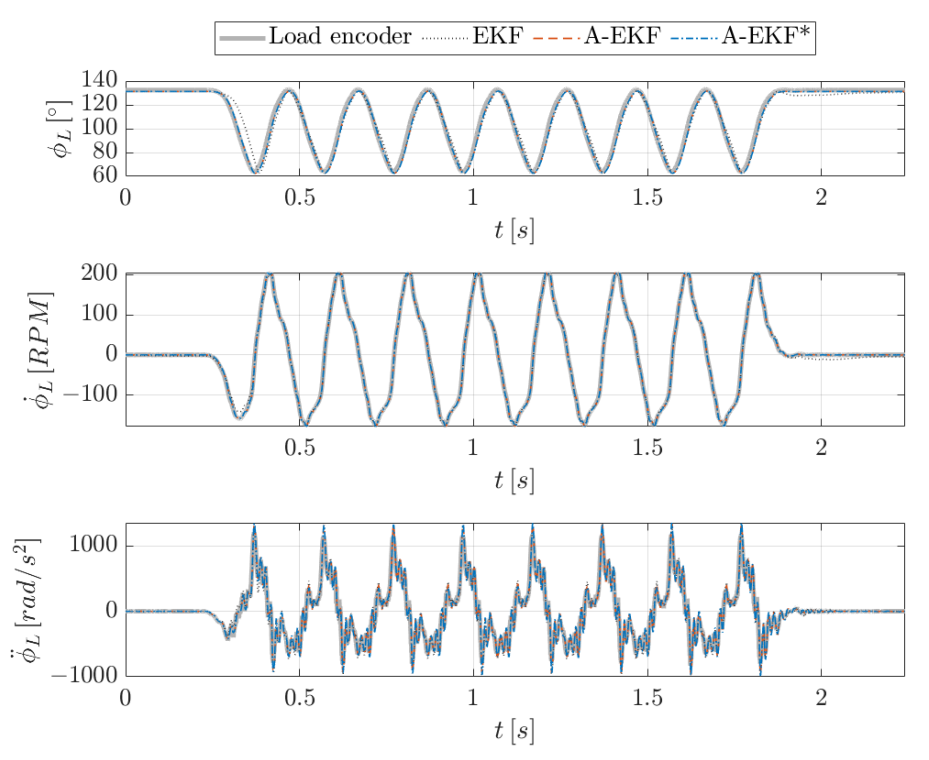
  • Extended Kalman filter (EKF) without augmented states where the magnetic spring torque input is modelled as an additional uncertainty. As such, the input torque is not estimated;
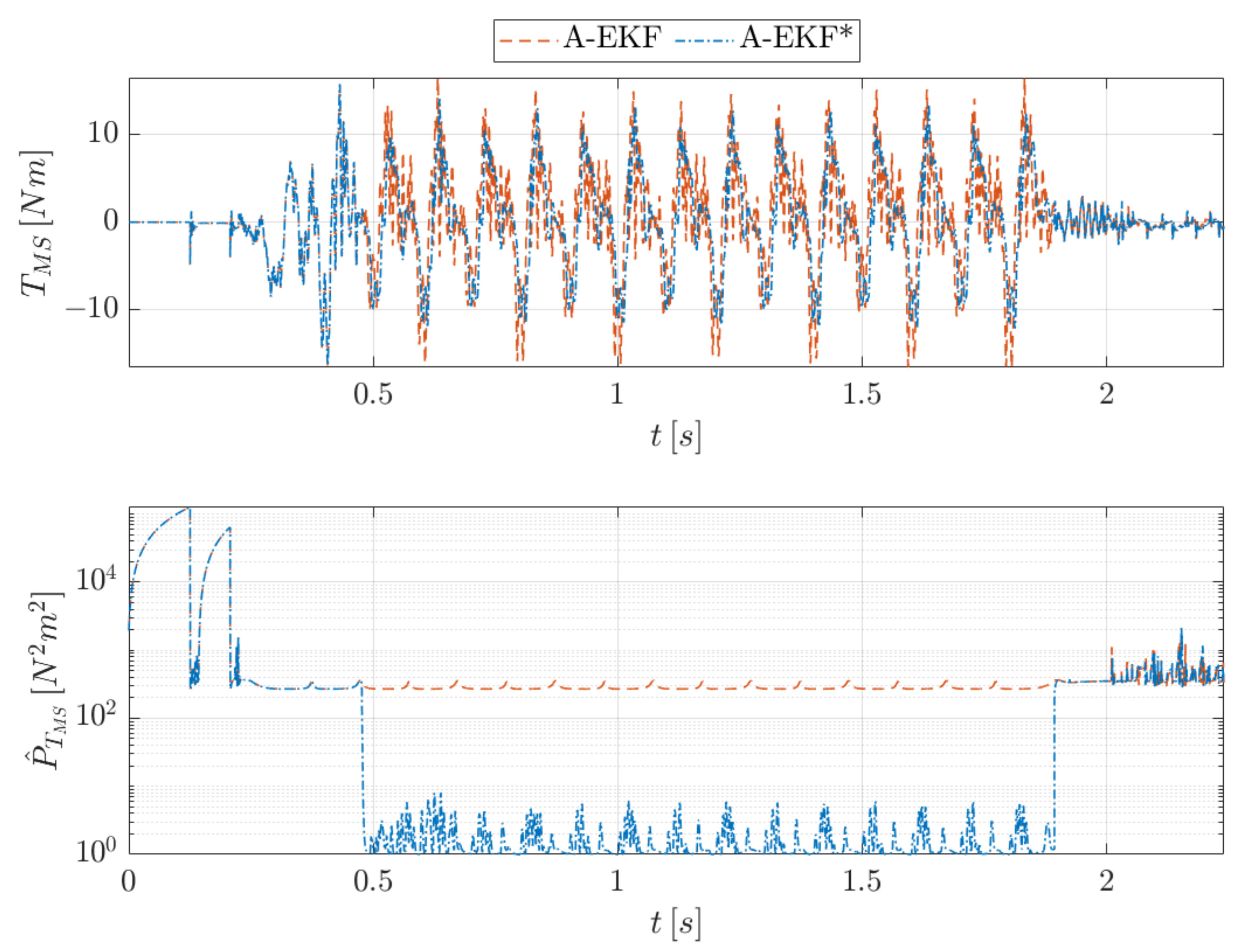
  • Augmented extended Kalman filter (A-EKF) where the augmented state for the magnetic spring torque input is modelled using a random walk model, without exploitation of the periodicity;
  • The proposed augmented extended Kalman filter, where the torque input model has an adaptive random walk covariance, depending on the gradient of the angle-dependent torque map (referred to as A-EKF*).
The motor angle, speed, and acceleration of the three different approaches are compared to the motor encoder signal in Figure 3. Regarding the angle estimation, all three approaches have a close match with the measured angle. For the motor rotational speed, the A-EKF and A-EKF* estimators that include the magnetic input torque estimation outperform the EKF that incorporates it as an uncertainty.
The difference is even more pronounced in the plot of the rotational acceleration. In order to allow a differentiation between the A-EKF and the A-EKF* approaches, the acceleration bounds are too limited to show the complete range of accelerations resulting from the EKF approach. However, the plot clearly shows the advantage of including the magnetic spring torque input in the estimation.
It can also be seen in the plot that the accelerations of the A-EKF and A-EKF* are aligned in the first-time interval. At t 0.5 s, the signals start to differ. This can be declared by the adaptive random walk covariance calculation of the A-EKF* approach. In the beginning, it is a constant value, equal to the constant random walk covariance of the A-EKF. Then, at t 0.5 s, it starts adapting the value using the gradient of the constructed torque map. As such, the random walk covariance is reduced when allowed by the calculation, and the calculated acceleration values are less extreme for the A-EKF* as compared to the A-EKF case. The motor acceleration is most accurate for the A-EKF* approach, as can be seen by comparing it to the differentiated encoder signal.
The load angle, speed, and acceleration of the three different approaches are compared to the load encoder signal in Figure 4. For the EKF approach, a delay is observed in the first cycle of the load angle. For the load rotational speed, all three estimations correspond well with the measured speed of the load encoder, although a slight mismatch can be observed at a few time intervals for the EKF. For the load rotational acceleration, the general trend of the three approaches and the differentiated encoder signal is similar. This is not surprising, as all three approaches use the same load accelerometer and the same model. The differences in the estimation approaches are at the motor side, with only a limited effect on the estimation of the end effector acceleration.
The estimated magnetic spring torque and its corresponding variance value are plotted in Figure 5. This input torque is only estimated in the A-EKF and A-EKF*, and no reference signal is easily available. Firstly, the two estimations are the same, as the adaptive random walk covariance calculation is not active yet. Starting at t 0.5 s, the A-EKF* adapts the random walk covariance using the gradient value of the torque map, leading to a smoother and more limited in amplitude magnetic spring torque estimation. The reduction in random walk covariance causes the state variance of the magnetic spring torque to decrease in amplitude as well. At the end of the run, the mechanism brakes, causing the magnetic spring torque to decrease as well. The A-EKF* detects this gradient and deactivates the adaptive covariance calculation of the random walk model, as the torque map no longer provides valuable information.
Figure 6 shows the torque at the load inertia and its corresponding estimated variance during two steady-state cycles ( t = [ 1.2 s , 1.6 s ] ). The estimated torque is compared to two reference signals that are obtained by multiplying the load acceleration signals derived from the sensor outputs with the load inertia value. The observed difference between the approaches is limited for the load torque estimation, as they differ only in the magnetic spring torque estimation at the motor side.
The corresponding variance, however, shows more obvious differences among the approaches. In order to declare these differences, the variance characteristic should firstly be understood for one approach. For this reason, the discussion starts with the explanation of the variance characteristic for the A-EKF approach. After this explanation, the differences with the EKF and A-EKF* approach are described.
The observed load torque variance is quasiperiodic for the A-EKF. When comparing this variance to the corresponding load angle, it can be noted that:
(i)
The variance reaches local minima when the load inertia reaches its reciprocating point (either minimal or maximal load angle);
(ii)
The variance reaches local maxima when the load inertia crosses its zero point (zero load angle).
This behaviour is due to the kinematics of the four-bar linkage and can be declared by considering the changing sensitivity of the rocker angle to the crank angle (quantified by ϕ θ ) at the two events:
(i)
The sensitivity is minimal; hence, the uncertain crank angle has only a limited influence on the uncertainty of the rocker angle;
(ii)
The sensitivity is maximal; hence, the uncertain crank angle has a more severe influence on the uncertainty of the rocker angle.
The relatively high uncertainty value of the crank angle results from the linear spring-damper connection with the motor inertia on which the highly uncertain magnetic spring torque is introduced. Considering that the connection between the rocker inertia and the load inertia is modelled in a similar fashion, it should not be surprising that the uncertainty of the rocker angle plays an important role for the load torque variance.
The variance obtained with the EKF shows a very similar behaviour, although it is hardly visible on Figure 6 because of the small amplitude of this variation in comparison with the other approaches. Due to the higher uncertainty value on the motor inertia equation in the EKF approach, the estimation relies almost entirely on the accelerometers and less on the model and the motor encoder. This results in a higher and more constant variance characteristic.
The A-EKF* reduces the variance of the magnetic spring torque input by exploiting its angle-dependency, and as such, the resulting load torque variance is also reduced compared to the A-EKF. This reduction is more significant for the originally highest variance values, as expected based on the corresponding higher sensitivity of rocker angle to crank angle.
Figure 7 shows a histogram of the error between the estimated load torque and the encoder reference. A normal distribution is fitted on the error data and can be compared to the theoretical error distribution. The theoretical distribution is a zero-mean normal distribution, with a variance value σ t h = σ e n c o d e r n o i s e 2 + σ e s t i m a t o r 2 (the noise variance of the load encoder reference is identified as σ e n c o d e r n o i s e = 0.99 based on its relative error distribution with the load accelerometer).
For the EKF approach, the error distribution shows a significant bias. This bias is reduced by including the magnetic spring torque in the estimation in the A-EKF. The A-EKF* approach allows one to reduce this bias even more by adapting the random walk covariance of the magnetic spring. This adaptation reduces the predicted uncertainty in the estimator, yielding the lowest theoretical variance value of the three approaches. However, the error standard deviation relative to the encoder reference is the highest of the three approaches. The A-EKF approach achieves the lowest error standard deviation relative to the encoder.
Regarding the interpretation and added value of the results here, it is important to bear in mind the limitations:
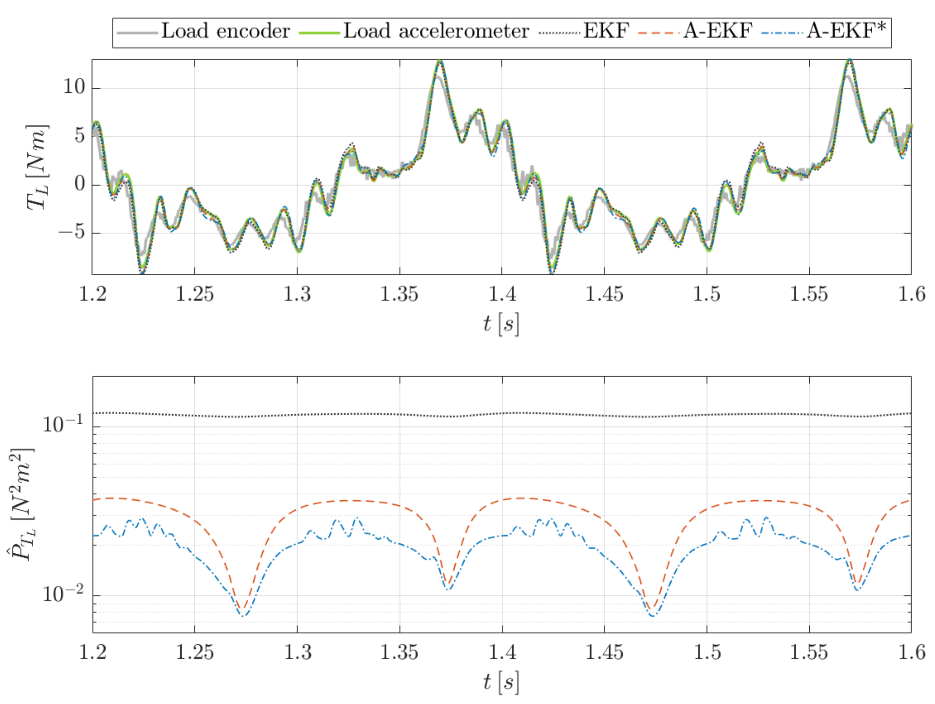
  • The main difference between the estimation approaches is in the estimation of the magnetic spring torque at the motor side, while the comparison of the results is performed at load side. This may declare the relatively limited difference for this comparison;
  • The comparison of the estimation errors relative to the independent encoder reference has a certain value. However, its value should not be overestimated as the encoder has a limited accuracy, and the comparison between the approaches may yield different results when a different validation sensor is used;
  • It is assumed that the load torque is known by multiplying the acceleration value of the sensor or the estimator with the load inertia value, as it is assumed no external torques are active on the inertia. A more extensive validation using a torque sensor would allow one to validate this assumption.

5. Conclusions

This paper proposes a nonintrusive estimation approach to identify the torsional loading on a mechatronic drivetrain. A combined state/input estimation using an augmented extended Kalman filter (A-EKF) combined a physics-based lumped parameter model of the torsional dynamics of the drivetrain with measurements coming from a motor encoder and two MEMS accelerometers. The installed magnetic spring allows one to reduce the torsional vibrations and improve the actuator performance, while posing additional challenges on the identification. In order to allow a generic magnetic spring torque estimation, a random walk input model is used, where the periodic angle-dependent behaviour is exploited to reduce the uncertainties on the estimates. As such, the proposed approach provided knowledge of the torsional vibrations, without the need for an extensive magnetic spring torque identification.
The results of the applied input estimation approach were compared to two alternative approaches, i.e., modelling the input as an additional uncertainty and estimating the input as a regular augmented model. The obtained load torque estimates were experimentally validated by comparing them to the signal of an independent high-resolution optical encoder at the load inertia. The results showed that a concurrent input estimation allows one to limit the bias in the load torque estimation. Furthermore, exploiting the periodic angle-dependency of the input allows one to significantly reduce the estimation variance.

Author Contributions

Conceptualization, T.V.d.V., M.K. and J.C.; methodology, T.V.d.V. and J.C.; implementation, T.V.d.V.; instrumentation and data acquisition T.V.d.V., J.B. and J.C.; validation, T.V.d.V. and J.C.; resources, J.B. and W.D.; writing—original draft preparation, T.V.d.V.; writing—review and editing, J.C., M.K. and F.N.; supervision, J.C. and M.K.; project administration, M.K.; funding acquisition, W.D. All authors have read and agreed to the published version of the manuscript.

Funding

This research was partially supported by Flanders Make, the strategic research center for the manufacturing industry. Internal Funds KU Leuven and VLAIO (Flanders Innovation and Entrepreneurship Agency) are also gratefully acknowledged for their support.

Institutional Review Board Statement

Not applicable.

Informed Consent Statement

Not applicable.

Data Availability Statement

The data presented in this paper result from activities within the acknowledged project and are available therein.

Conflicts of Interest

The authors declare no conflict of interest.

References

  1. Nordström, L.J.L.; Nordberg, T.P. A critical comparison of time domain load identification methods. In Proceedings of the 6th International Conference on Motion and Vibration Control, Saitama, Japan, 19–23 August 2002; pp. 1151–1156. [Google Scholar]
  2. Klinkov, M.; Fritzen, C.P. An updated comparison of the force reconstruction methods. Key Eng. Mater. 2007, 347, 461–466. [Google Scholar] [CrossRef]
  3. Kalman, R.E. A New Approach to Linear Filtering and Prediction Problems. Trans. ASME J. Basic Eng. 1960, 82, 35–40. [Google Scholar] [CrossRef] [Green Version]
  4. Kalman, R.E.; Bucy, R.S. New results in linear filtering and prediction theory. Trans. ASME J. Basic Eng. 1961, 83, 95–108. [Google Scholar] [CrossRef]
  5. Lourens, E.; Reynders, E.; De Roeck, G.; Degrande, G.; Lombaert, G. An augmented Kalman filter for force identification in structural dynamics. Mech. Syst. Signal Process. 2012, 27, 446–460. [Google Scholar] [CrossRef]
  6. Naets, F.; Croes, J.; Desmet, W. An online coupled state/input/parameter estimation approach for structural dynamics. Comput. Methods Appl. Mech. Eng. 2014, 283, 1167–1188. [Google Scholar] [CrossRef]
  7. Croes, J. Virtual Sensing in Mechatronic Systems. Ph.D. Thesis, KU Leuven, Leuven, Belgium, 2017. [Google Scholar]
  8. Forrier, B.; Naets, F.; Desmet, W. Broadband Load Torque Estimation in Mechatronic Powertrains using Nonlinear Kalman Filtering. IEEE Trans. Ind. Electron. 2018, 65, 2378–2387. [Google Scholar] [CrossRef]
  9. Kirchner, M. Joint State/Input Estimation in Structural Dynamics. Ph.D. Thesis, KU Leuven, Leuven, Belgium, 2018. [Google Scholar]
  10. Kirchner, M.; Croes, J.; Cosco, F.; Desmet, W. Exploiting input sparsity for joint state/input moving horizon estimation. Mech. Syst. Signal Process. 2018, 101, 237–253. [Google Scholar] [CrossRef]
  11. Kirchner, M.; Croes, J.; Desmet, W. Joint state/input estimation with a Fourier dictionary for the input respresenation: Effect of spectral leakage. In Proceedings of the 13th International Conference on Recent Advances in Structural Dynamics, Lyon, France, 15–17 April 2019; pp. 370–381. [Google Scholar]
  12. Mrak, B.; Lenaerts, B.; Driesen, W.; Desmet, W. Optimal Magnetic Spring for Compliant Actuation—Validated Torque Density Benchmark. Actuators 2019, 8, 18. [Google Scholar] [CrossRef] [Green Version]
  13. Mrak, B.; Lenaerts, B.; Driesen, W.; Desmet, W. Optimal Design of Magnetic Springs; Enabling High Life Cycle Elastic Actuators. In Proceedings of the 16th International Symposium on Magnetic Bearings, Beijing, China, 13–17 August 2018. [Google Scholar]
  14. McCarthy, J.; Soh, G. Geometric Design of Linkages, 2nd ed.; Springer: New York, NY, USA, 2011. [Google Scholar]
  15. Simon, D. Optimal State Estimation, 1st ed.; John Wiley & Sons: Hoboken, NJ, USA, 2006; pp. 395–433. [Google Scholar]
  16. Bar-Shalom, Y.; Li, X.R. Estimation and Tracking: Principles, Techniques, and Software, 1st ed.; Artech House: Boston, MA, USA; London, UK, 1993. [Google Scholar]
Figure 1. Schematic representation of the mechatronic powertrain model.
Actuators 11 00035 g001
Figure 2. Experimental test setup.
Actuators 11 00035 g002
Figure 3. Estimated and reference motor angle, speed, and acceleration.
Actuators 11 00035 g003
Figure 4. Estimated and reference load angle, speed, and acceleration.
Actuators 11 00035 g004
Figure 5. Estimated magnetic spring torque and variance.
Actuators 11 00035 g005
Figure 6. Estimated and reference load torque and variance.
Actuators 11 00035 g006
Figure 7. Error between estimated and reference load torque: histogram and normal data fit for the three estimation approaches. Comparison with theoretical distribution.
Actuators 11 00035 g007
Publisher’s Note: MDPI stays neutral with regard to jurisdictional claims in published maps and institutional affiliations.

