Research on Trajectory Tracking of Sliding Mode Control Based on Adaptive Preview Time

Abstract

The preview model is one of the common methods used in trajectory tracking. The traditional fixed preview time is not adaptable to most speeds and road conditions, which not only reduces the tracking accuracy but also reduces the vehicle stability. Therefore, a controller can be designed to determine the adaptive preview time based on an optimization function of the lateral deviation, the road boundary, and the road boundary of the whole vehicle motion response characteristics. Traditional optimal preview control theory predicts the next state of the vehicle by the assumption of constant transverse pendulum angular velocity. In this paper, an expectation-based approach is used to find the ideal steering wheel turning angle based on the adaptive preview time, and a single-point preview model is established. Based on the two-degree-of-freedom dynamics model, a sliding mode controller is designed for control, and the low-pass filters are designed to suppress jitter in the sliding mode controller. Simulation results with different preview times, different speeds and different road adhesion coefficients prove that the controller has a good control effect and has good effectiveness and adaptability to speed and adhesion coefficient.

1. Introduction

The autonomous vehicle is a new future concept that fulfills people’s vision of the future. It is an integrated system that brings together environmental perception, planning and decision-making, and control execution, integrating technologies such as sensors, information interaction, artificial intelligence, automatic control, and traditional vehicles, and is an innovative embodiment of cross-fertilization of disciplines [1]. Trajectory tracking is an indispensable part of control execution technology, which relies on the underlying control technology of the vehicle and also requires good tracking of the planned trajectory, and good tracking effect has important significance for the safety and control of intelligent vehicles, which can reduce the probability of traffic accidents due to driver negligence and can reduce the dependence of previous vehicles on driver operation. The preview follower theory can accurately reflect the driver’s control behavior [2], and the lateral position deviation of the preview point position from the desired trajectory can be obtained based on the two-degree-of-freedom vehicle dynamic model, and then the ideal yaw rate which is used to provide input for the sliding mode controller can be calculated.

The current research in the field of vehicle control focuses on establishing an efficient and reasonable lateral stability control strategy [3], and the main lateral control algorithms include classical PID (Proportional Integral Derivative) control methods [4], optimal preview control methods [5,6], robust control [7], sliding mode control methods [8], modern control algorithm MPC (Model Predictive Control) methods [9,10], fuzzy control methods [11], and so on, and the optimization strategies of various methods are innumerable. The literature uses lane line detection techniques combined with model predictive control to design controllers [12]; uses particle swarms to optimize higher-order sliding mode control parameters [13]; and designs controllers based on adaptive preview with directional error compensation [14].

The principle of sliding mode control is to design the switching plane of the system according to the desired dynamic characteristics of the system. This plane represents the steady state of the system, after which the system state is made to converge from out of plane to the switching plane by means of a sliding mode controller. Zhang et al. [15] designed a path tracking control strategy with strong robustness and without chattering based on a sliding mode technique with conditional integrators. Exact linear transformation method was used by Zhang et al. [16] to linearize the system model and a sliding-mode controller was designed for the trajectory tracking of semi-trailer vehicles in automatic reversing. In order to improve the longitudinal motion control accuracy of intelligent vehicles, the RBF (Radial Basis Function) neural network adaptive sliding mode control strategy was used by Hui Yijia [17] to control the longitudinal dynamics of intelligent vehicles.

Although the sliding mode control method is prone to jitter, it also has more advantages such as being insensitive to perturbations of parameter changes, more resistant to disturbances, more robust, and can respond quickly. In this paper, the ideal angular velocity of the transverse pendulum is obtained using the preview point, and the sliding mode controller is designed to perform the control.

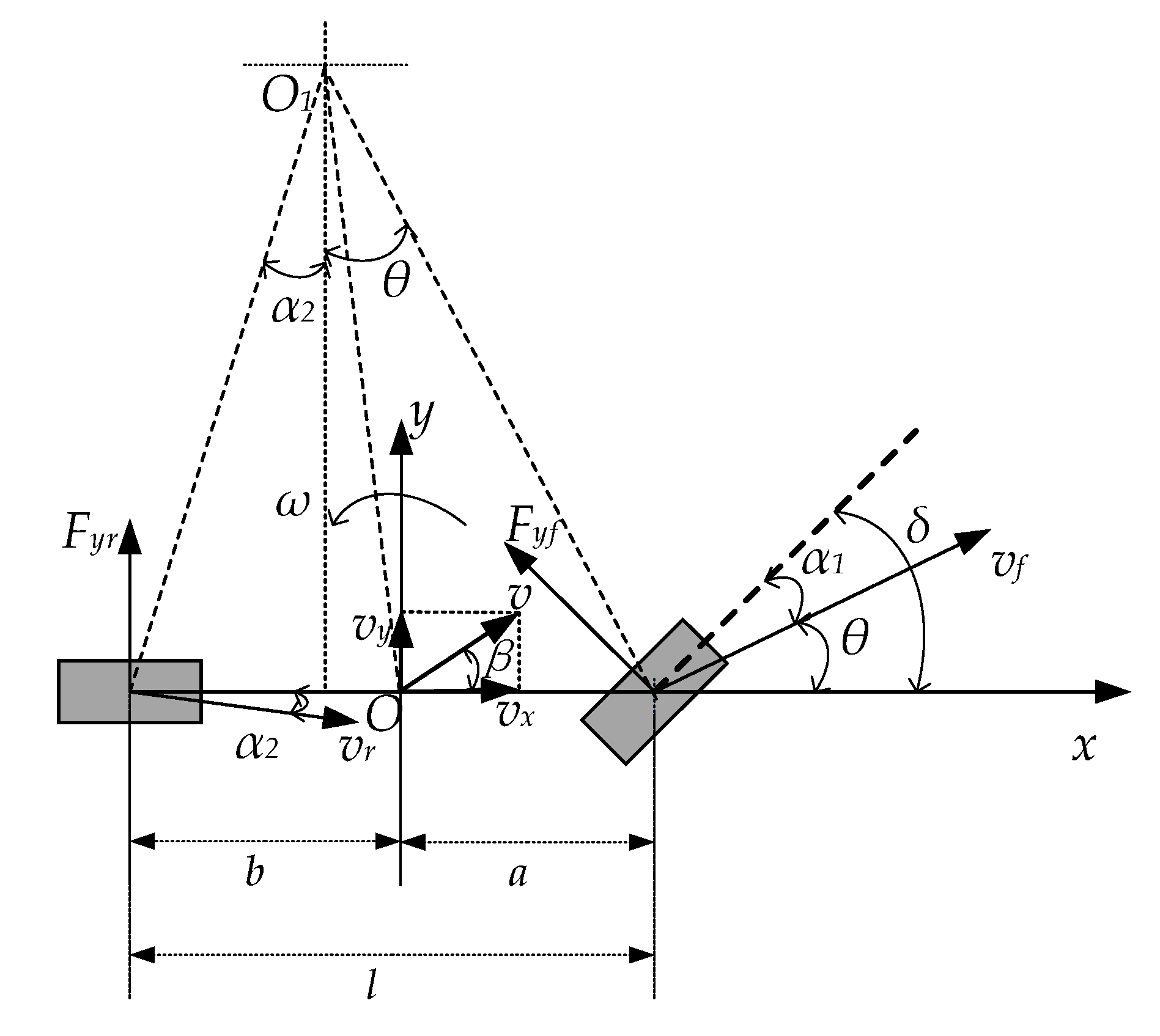
2. Vehicle Dynamics Model

The vehicle dynamics model can be used to study the handling stability as well as the smoothness of the ride, and it is used in the field of trajectory tracking to perform stability studies. The dynamics model is modeled using two-degree-of-freedom dynamics, which is simplified to a bicycle model [18], as shown in Figure 1. In this Figure: a is the distance from the center of mass to the front axle; b is the distance from the center of mass to the rear axle; F_yf is the lateral force of the front wheel; F_yr is the lateral force of the rear wheel; v_x is the longitudinal speed; v_y is the lateral speed; ω is the angular velocity of transverse pendulum; β is the lateral deflection angle of the center of mass.

Assuming that the front wheels of the vehicle rotate at a small angle, the dynamic equation of vehicle centroid is established, and the set of equations is as follows [19]:

$$\left\{\begin{array}{c}\mathit{m}{\dot{\mathit{v}}}_{\mathit{x}}{+\mathit{mv}}_{\mathit{x}}{\mathit{\omega }=\mathit{F}}_{\mathit{yf}}+{\mathit{F}}_{\mathit{yr}}\\ {\mathit{I}}_{\mathit{z}}\dot{\mathit{\omega }}={\mathit{aF}}_{\mathit{yf}}{-\mathit{bF}}_{\mathit{yr}}\end{array}\right.$$

(1)

where m is the mass of the whole vehicle, I_z is the rotational inertia of the vehicle at the center of mass, ${\dot{\mathit{v}}}_{\mathit{x}}$ is the lateral acceleration, $\dot{\mathit{\omega }}$ is the angular acceleration of the transverse pendulum.

Supposing the front wheel of the vehicle rotates at a small angle, the relationship between lateral deflection force, lateral deflection angle and lateral deflection stiffness when the tire is in the linear region can be expressed as follows:

$$\{\begin{array}{c}{\mathit{F}}_{\mathit{yf}}{=\mathit{C}}_{\mathit{f}}{\mathit{\alpha }}_{\mathit{f}}\\ {\mathit{F}}_{\mathit{yr}}{=\mathit{C}}_{\mathit{r}}{\mathit{\alpha }}_{\mathit{r}}\end{array}$$

(2)

where ${\mathit{C}}_{\mathit{f}}$ ${\mathrm{and} \mathit{C}}_{\mathit{r}}$ are the front wheel lateral deflection stiffness and rear wheel lateral deflection stiffness respectively,${ \mathit{\alpha }}_{\mathit{f}}$ and ${\mathit{\alpha }}_{\mathit{r}}$ are front wheel lateral deflection angle and rear wheel lateral deflection angle. The front wheel side deflection angle and the rear wheel side deflection angle of the vehicle is related to its motion parameters. Assuming that the velocities of the front and rear axles of the vehicle are ${\mathit{v}}_{\mathit{x}}$ and ${\mathit{v}}_{\mathit{y}}$ respectively, lateral deflection angle of the center of mass is $\mathit{\beta }$,$\mathit{\beta }=\mathit{arctan}\left(\frac{{\mathit{v}}_{\mathit{y}}}{{\mathit{v}}_{\mathit{x}}}\right)\approx \frac{{\mathit{v}}_{\mathit{y}}}{{\mathit{v}}_{\mathit{x}}}$.

The angle between the direction of velocity of the front wheel and the x-axis is θ, which can be expressed as follows:

$$\mathit{\theta }=\frac{{\mathit{v}}_{\mathit{y}}+\mathit{\omega }\mathit{a}}{{\mathit{v}}_{\mathit{x}}}=\mathit{\beta }+\frac{\mathit{\omega }\mathit{a}}{{\mathit{v}}_{\mathit{x}}}$$

(3)

The lateral deflection angle of the front and rear wheels of vehicle in Figure 1 can be expressed as follows:

$$\{\begin{array}{c}{\mathit{\alpha }}_{\mathit{f}}=\mathit{\beta }+\frac{\mathit{\omega }\mathit{a}}{{\mathit{v}}_{\mathit{x}}}-\mathit{\delta }\\ {\mathit{\alpha }}_{\mathit{r}}=\mathit{\beta }-\frac{\mathit{\omega }\mathit{b}}{{\mathit{v}}_{\mathit{x}}}\end{array}$$

(4)

The model equations for the two degrees of freedom of the vehicle with respect to the transverse pendulum angle ω and the lateral declination angle β of the center of mass can be obtained by Equations (1), (2) and (4):

$$\left[\begin{array}{c} \dot{\mathit{\beta }}\\ \dot{\mathit{\omega }}\end{array}\right]=\left[\begin{array}{cc}\frac{{\mathit{C}}_{\mathit{f}}{+\mathit{C}}_{\mathit{r}}}{{\mathit{mv}}_{\mathit{x}}}& \frac{{\mathit{aC}}_{\mathit{f}}{-\mathit{bC}}_{\mathit{r}}}{{\mathit{mv}}_{\mathit{x}}}-1\\ \frac{{\mathit{aC}}_{\mathit{f}}{-\mathit{bC}}_{\mathit{r}}}{{\mathit{I}}_{\mathit{z}}}& \frac{{\mathit{a}}^2{\mathit{C}}_{\mathit{f}}{+\mathit{b}}^2\mathit{Cr}}{{\mathit{I}}_{\mathit{z}}{\mathit{v}}_{\mathit{x}}}\end{array}\right]\left[\begin{array}{c}\mathit{\beta }\\ \mathit{\omega }\end{array}\right]-\left[\begin{array}{c}\frac{{\mathit{C}}_{\mathit{f}}}{{\mathit{mv}}_{\mathit{x}}}\\ \frac{{\mathit{aC}}_{\mathit{f}}}{{\mathit{I}}_{\mathit{z}}}\end{array}\right]\mathit{\delta }$$

(5)

3. Adaptive Preview Model

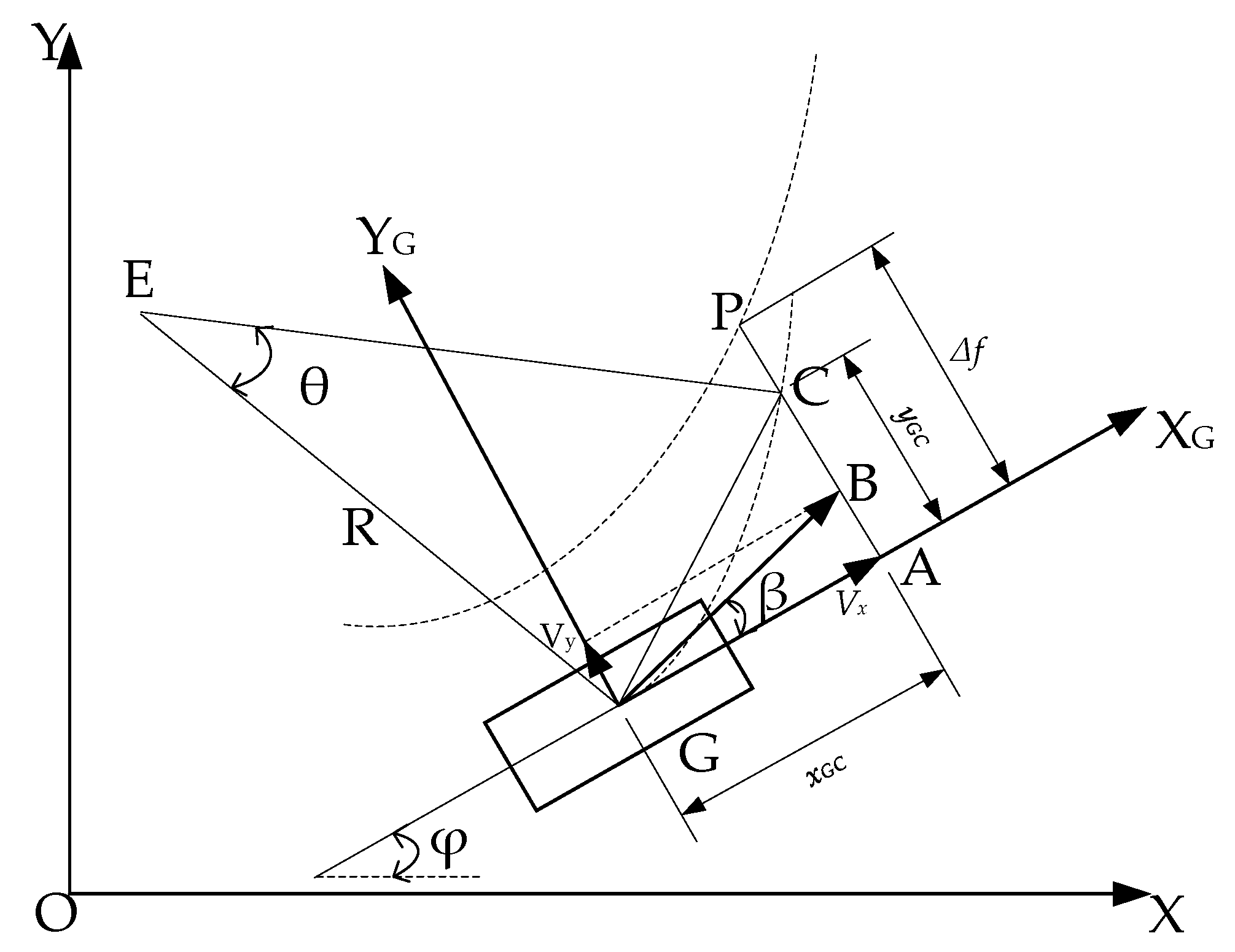
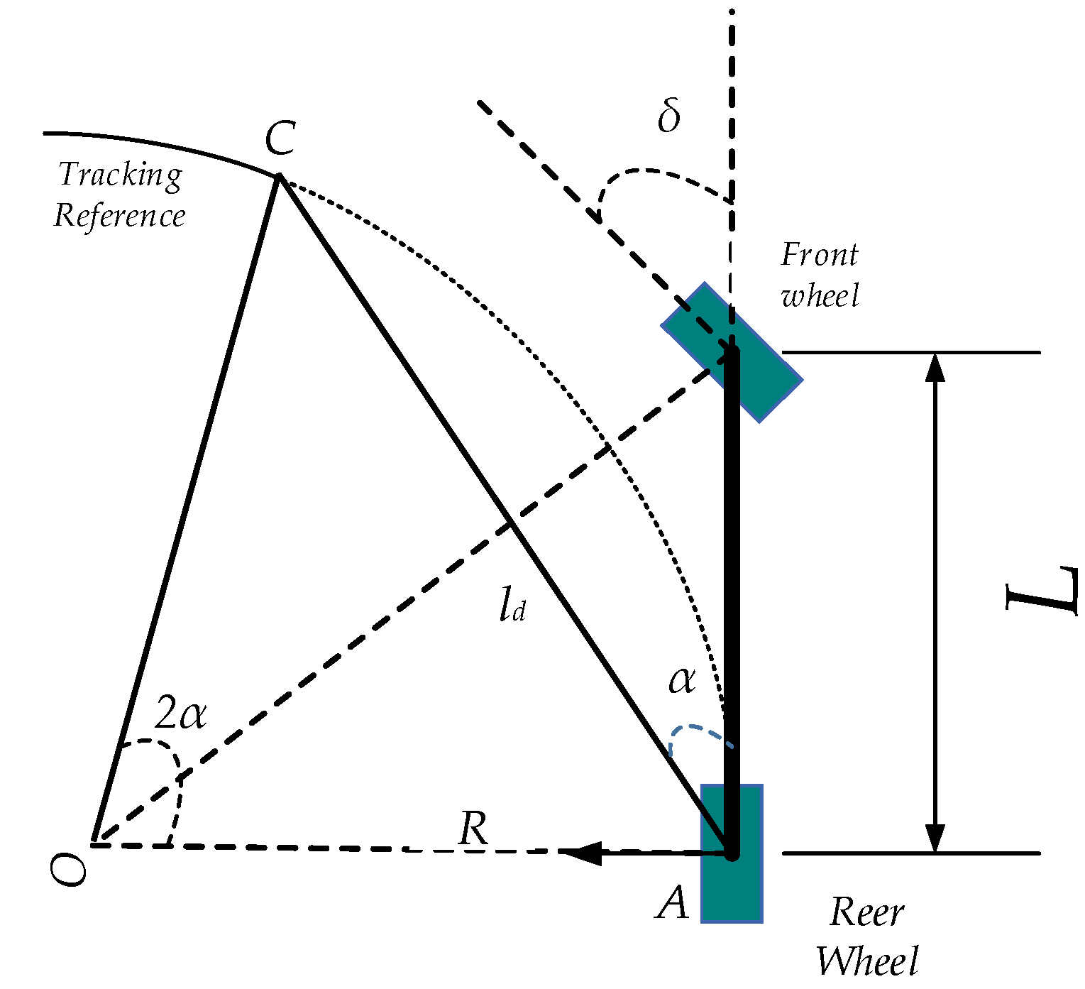
3.1. Optimal Curvature Single Point Preview

The ideal steering wheel turning angle is decided by the expectation-based method [20], and a constant transverse pendulum angular velocity assumption is made, as shown in Figure 2. The predicted trajectory is treated as a circle with point E as the center and radius R, and the angle of the center of the circle is θ.

In Figure 2, XOY is inertial coordinate system; X_G-Y_G is body coordinate system; point G is the position of the center of mass of the vehicle; point C is the predicted position after t_p time; point P is the preview point on the target trajectory; Δf is the lateral deviation; x_GC and y_GC are the displacements in the X_G and Y_G directions after t_p time; φ is the vehicle heading angle; β is the mass lateral deviation angle; and v is the vehicle travel speed.

The ideal angular velocity of the transverse pendulum ${\mathit{\omega }}_{\mathit{d}}$ can be expressed as follows:

$${\mathit{\omega }}_{\mathit{d}}=2\left[\mathit{arctan}\right(\frac{\mathsf{\Delta }\mathit{f}}{{\mathit{v}}_{\mathit{x}}{\mathit{t}}_{\mathit{p}}}{)-\mathit{\beta }]\mathit{t}}_{\mathit{p}}^{-1}$$

(6)

Parameter ${\mathit{\omega }}_{\mathit{d}}$ is calculated under the assumption of steady-state transverse pendulum angular velocity, so there is a slight deviation from the theoretical one. During the simulation, it was found that the magnitude of ${\mathit{\omega }}_{\mathit{d}}$ is related to the velocity, and after extensive simulation verification, the formula for calculating ${\mathit{\omega }}_{\mathit{d}}$ was adjusted as follows:

$${\mathit{\omega }}_{\mathit{d}}=(2+0.04\ast {\mathit{v}}_{\mathit{x}}\left)\right[\mathit{arctan}(\frac{\mathsf{\Delta }\mathit{f}}{{\mathit{v}}_{\mathit{x}}{\mathit{t}}_{\mathit{p}}}{)-\mathit{\beta }]\mathit{t}}_{\mathit{p}}^{-1}$$

(7)

3.2. Adaptive Preview Time

By selecting different preview time t_p, the driver is simulated to adapt to different road conditions to attain the preview distance, and the general preview time is selected in the range of 0.3–1.5 s.

L_Drv_2 is the lateral offset of the current center of mass and the distance between the actual trajectory, designing the cost function according to L_Drv_2 considering tracking accuracy [21,22]:

$${\mathit{J}}_1={{\displaystyle \int }}_0^{\mathit{t}}{\mathit{L}\_\mathit{Drv}\_2}^2\mathit{dx}$$

(8)

where L_Drv_2 is the lateral offset, t is model prediction time.

In order to satisfy the boundary constraints, the driver model must design an optimization function for the distance between the trajectory and the boundary location to ensure that the vehicle can safely cross the road:

$$J_2={{\displaystyle \int }}_0^{t}gdx$$

(9)

where g is security functions, the closer the vehicle position is to the boundary, the larger the g value. g is calculated:

$$\mathit{g}=\frac{\left|\frac{\mathit{L}\_\mathit{Drv}\_2}{1.75-\mathit{L}\_\mathit{Drv}\_2}\right|}{1-|\frac{\mathit{L}\_\mathit{Drv}\_2}{1.75-\mathit{L}\_\mathit{Drv}\_2}|}$$

(10)

where L_Drv_2 is the lateral offset, the width of the road is set at 3.5 m.

When designing the preview time, the dynamic response time characteristics of the steering motion of the vehicle also need to be taken into account:

$${\mathit{J}}_3=\frac{1}{8}{\left({\mathit{t}}_{\mathit{p}}-\mathit{T}\right)}^2$$

(11)

where T is time associated with vehicle steering response characteristics, it can be taken as 1 s or shorter when the speed is high, and can be increased when the speed is low.

Combining the above optimization functions, the optimization function is obtained as:

$$J=\mathit{min}\left({\mathit{\omega }}_1{\mathit{J}}_1{+\mathit{\omega }}_2{\mathit{J}}_2{+\mathit{\omega }}_3{\mathit{J}}_3\right)$$

(12)

where ${\mathit{\omega }}_1,{\mathit{\omega }}_2,{\mathit{\omega }}_3$ is weight factor, the setting of weights is related to the purpose achieved, ${\omega }_1$ is related to the accuracy of trajectory tracking; ${\mathit{\omega }}_2$ is related to the distance between the vehicle and the road boundary; ${\mathit{\omega }}_3$ is related to the response characteristics of the whole vehicle.

The range of preview is from 0.3 s to 1.5 s; this study has designed a multiple criteria optimization with three selection principles to select the best preview time. The method the study used is an iterative method which through the array [0.3,1.5] with a step size of 0.01 s, to find the smallest J at each moment ($J=min\left({\omega }_1{J}_1+{\omega }_2{J}_2+{\omega }_3{J}_3\right)$). The values of the three weighting parameters are ω₁ = 0.2; ω₂ = 0.05; ω₃ = 0.75.

4. Design of Sliding Mode Controller

By combining the advantages of sliding mode control and the preview control algorithm, a sliding mode controller based on preview control is designed, which can reflect both the driver’s operating characteristics and boundary constraints, as well as the motion response characteristics of the whole vehicle. The controller is insensitive to the perturbation of parameter changes, with better anti-interference capability and robustness, and also previews the path; in this way, it can guarantee the steering wheel rotation stability, improve the tracking effect of the trajectory tracking control algorithm, and enhance the accuracy of the tracking controller [23]. The design diagram of the sliding mode controller is shown in Figure 3, the parameters in the Figure 3 are described in detail in the derivation of the equations later.

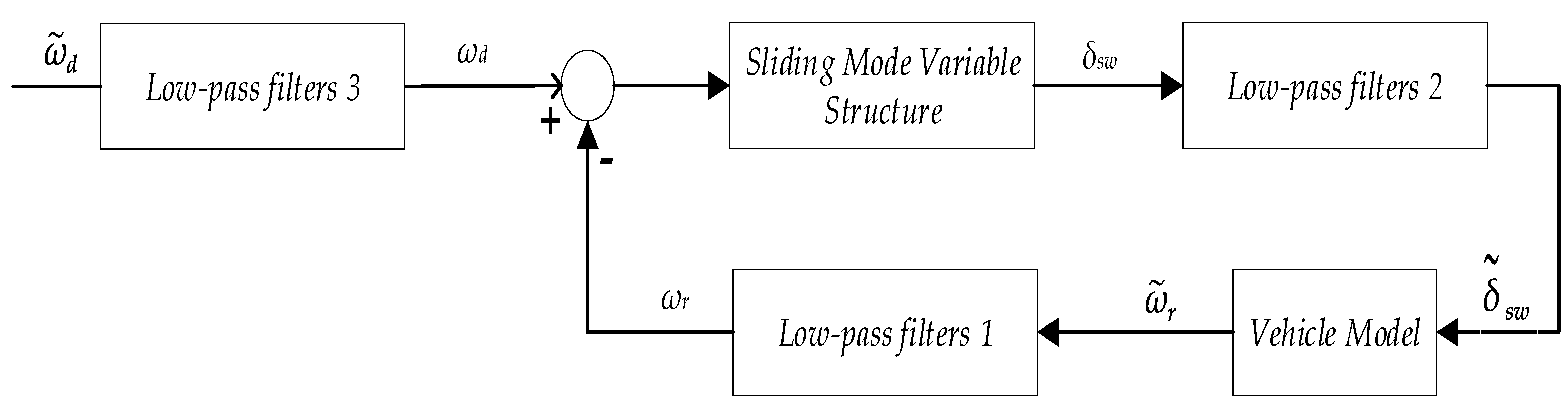
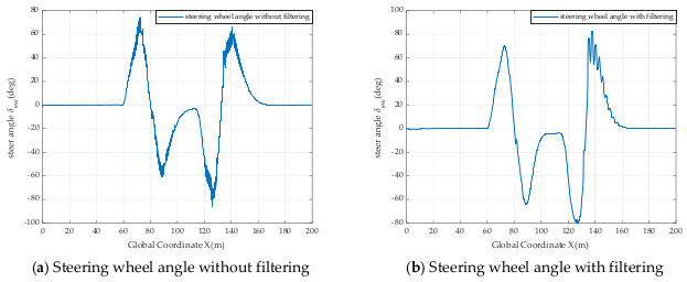
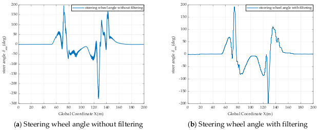
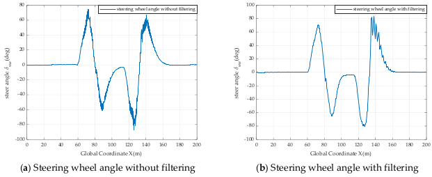
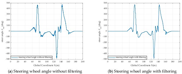
4.1. Design of Low-Pass Filters

Combining sliding mode control methods with filters enables filtering of noisy signals, providing a smooth signal for the sliding mode controller. The structure of a low-pass filter-based sliding mode controller control system is shown in the following diagram [23,24], where ${\tilde{\mathit{\omega }}}_{\mathit{r}}\left(\mathit{t}\right){, \mathit{\delta }}_{\mathit{sw}}\left(\mathit{t}\right)$ is input for control, ${\tilde{\mathit{\delta }}}_{\mathit{sw}}\left(\mathit{t}\right){,\mathit{\omega }}_{\mathit{r}}$ is output for control. To reduce jitter generated by the sliding mode controller, the low-pass filter is designed as follows:

$$\mathit{Q}\left(\mathit{s}\right)=\frac{\mathit{\xi }}{\mathit{s}+\mathit{\xi }}$$

(13)

From Figure 4, we can obtain:

$${\dot{\tilde{\mathit{\omega }}}}_{\mathit{d}}{+\mathit{\Phi }}_1{\tilde{\mathit{\omega }}}_{\mathit{d}}{=\mathit{\Phi }}_1{\mathit{\omega }}_{\mathit{d}}$$

(14)

$${\dot{\tilde{\mathit{\omega }}}}_{\mathit{r}}{+\mathit{\Phi }}_2{\tilde{\mathit{\omega }}}_{\mathit{r}}{=\mathit{\Phi }}_2{\mathit{\omega }}_{\mathit{r}}$$

(15)

$$\dot{\mathit{\tau }}+\mathit{\xi }\mathit{\tau }=\mathit{\xi }\mathit{u}$$

(16)

4.2. Design of Sliding Mode Control Law

For a system that is uncertain and needs to take into account the uptake of internal parameters as well as external disturbances, the system equation of state can be better formulated as:

$$\dot{\mathit{x}} =\mathit{A}-\mathsf{\Delta }\mathit{Ax}+\left(\mathit{B}-\mathsf{\Delta }\mathit{B}\right)\mathit{u}\left(\mathit{t}\right)+\left(\mathit{d}-\mathsf{\Delta }\mathit{d}\right)\mathit{f}$$

(17)

Equation (5) can be rewritten by Equation (17) as:

$$\mathit{x}=\mathrm{[}\begin{array}{c}\mathit{\beta }\\ \mathit{\omega }\end{array}\mathrm{]}$$

(18)

$$\mathit{A}=\mathrm{[}\begin{array}{cc}{\mathit{A}}_1& {\mathit{A}}_2\\ {\mathit{A}}_3& {\mathit{A}}_4\end{array}\mathrm{]}$$

(19)

$$\mathit{B}=\mathrm{[}\begin{array}{c}{\mathit{B}}_1\\ {\mathit{B}}_2\end{array}\mathrm{]}$$

(20)

where is ${\mathit{A}}_1=\frac{{\mathit{C}}_{\mathit{f}}{+\mathit{C}}_{\mathit{r}}}{{\mathit{mv}}_{\mathit{x}}}$, ${\mathit{A}}_2=\frac{{\mathit{aC}}_{\mathit{f}}{-\mathit{bC}}_{\mathit{r}}}{{\mathit{mv}}_{\mathit{x}}}-1$, ${\mathit{A}}_3=\frac{{\mathit{aC}}_{\mathit{f}}{-\mathit{bC}}_{\mathit{r}}}{{\mathit{I}}_{\mathit{z}}}$, ${\mathit{A}}_4=\frac{{\mathit{a}}^2{\mathit{C}}_{\mathit{f}}{+\mathit{b}}^2\mathit{Cr}}{{\mathit{I}}_{\mathit{z}}{\mathit{v}}_{\mathit{x}}}$, ${\mathit{B}}_1=-\frac{{\mathit{C}}_{\mathit{f}}}{{\mathit{mv}}_{\mathit{x}}}$, ${\mathit{B}}_2=-\frac{{\mathit{aC}}_{\mathit{f}}}{{\mathit{I}}_{\mathit{z}}}$.

The equation of the controlled system can be expressed as the following equation of the state:

$$\begin{gathered} { \dot{\mathit{\omega }}}_{\mathit{r}}=\left({\mathit{A}}_3-\mathsf{\Delta }{\mathit{A}}_3\right)\mathit{\beta }+\left({\mathit{A}}_4-\mathsf{\Delta }{\mathit{A}}_4\right){\mathit{\omega }}_{\mathit{r}}+\left({\mathit{B}}_2-\mathsf{\Delta }{\mathit{B}}_2\right)\mathit{\delta }+\left(\mathit{d}-\mathsf{\Delta }\mathit{d}\right)\mathit{f}= \\ {\mathit{A}}_3{\mathit{\beta }+\mathit{A}}_4{\mathit{\omega }}_{\mathit{r}}{+\mathit{B}}_2\mathit{\delta }-\left(\mathsf{\Delta }{\mathit{A}}_3\mathit{\beta }+\mathsf{\Delta }{\mathit{A}}_4{\mathit{\omega }}_{\mathrm{r}}+\mathsf{\Delta }{\mathit{B}}_2\mathit{\delta }+\mathsf{\Delta }\mathit{df}\right) \end{gathered}$$

(21)

The uncertainty of the system and imposed disturbances are expressed in terms of $\mathit{E}\left(\mathit{t}\right)$, which can be expressed as:

$$\mathit{E}\left(\mathit{t}\right)=\Delta {\mathit{A}}_3\mathit{\beta }+\Delta {\mathit{A}}_4{\mathit{\omega }}_{\mathit{r}}+\Delta {\mathit{B}}_2\mathit{\delta }+\Delta \mathit{df}$$

(22)

Taking Equation (22) into Equation (21), we get into Equation, we obtain:

$${ \dot{\mathit{\omega }}}_{\mathit{r}}{=\mathit{A}}_3{\mathit{\beta }+\mathit{A}}_4{\mathit{\omega }}_{\mathit{r}}{+\mathit{B}}_2\mathit{\delta }-\mathit{E}\left(\mathit{t}\right)$$

(23)

Taking Equation (23) into Equation (16), we obtain:

$${\mathit{A}}_3{\mathit{\beta }+\mathit{A}}_4{\mathit{\omega }}_{\mathit{r}}{+\mathit{B}}_2\mathit{\delta }-\mathit{E}\left(\mathit{t}\right){+\mathit{\xi }\mathit{\omega }}_{\mathit{r}}=\mathit{\xi }\mathit{u}$$

(24)

Transforming the formula provides:

$${\mathit{\omega }}_{\mathit{r}}=\frac{1}{{\mathit{A}}_4+\mathit{\xi }}\left({\mathit{\xi }\mathit{u}-\mathit{A}}_3{\mathit{\beta }-\mathit{B}}_2\mathit{\delta }+\mathit{E}\left(\mathit{t}\right)\right)$$

(25)

The difference between the actual transverse pendulum angular velocity ω_r and the ideal transverse pendulum angular velocity ω_d is chosen as the tracking error of this system:

$${\mathit{e}=\mathit{\omega }}_{\mathit{r}}{-\mathit{\omega }}_{\mathit{d}}$$

(26)

The switching function is selected as follows:

$$\mathit{s}=\mathit{e}+\mathit{\lambda }{{\displaystyle \int }}_0^{\mathit{t}}\mathit{e}\left(\mathit{\tau }\right)\mathit{d}\mathit{\tau }$$

(27)

where $\lambda$ is a positive integer.

Taking Equation (26) into Equation (27) and the derivative of Equation (27), we obtain:

$$\dot{\mathit{s}} = \dot{\mathit{e}} +\mathit{\lambda }\mathit{e}= {\dot{\mathit{\omega }}}_{\mathit{r}}- {\dot{\mathit{\omega }}}_{\mathit{d}}+\mathit{\lambda }\left({\mathit{\omega }}_{\mathit{r}}{-\mathit{\omega }}_{\mathit{d}}\right)$$

(28)

Taking Equations (23) and (25) into Equation (28), we obtain:

$${ \dot{\mathit{s}} =\mathit{A}}_3\mathit{\beta }+\left({\mathit{A}}_4+\mathit{\lambda }\right){\mathit{\omega }}_{\mathit{r}}{+\mathit{B}}_2\mathit{\delta }-\mathit{E}\left(\mathit{t}\right){\dot{\mathit{\omega }}}_{\mathit{d}}{-\mathit{\lambda }\mathit{\omega }}_{\mathit{d}}$$

(29)

Choosing a Lyapunov function candidate $\mathit{V}=\frac{1}{2}{\mathit{s}}^2$ and differentiating V with respect to time, we have:

$$\begin{gathered} \dot{\mathit{V}} =\mathit{s}\dot{\mathit{s}} =\mathit{s}\left({\mathit{A}}_3\mathit{\beta }+\left({\mathit{A}}_4+\mathit{\lambda }\right){\mathit{\omega }}_{\mathit{r}}{+\mathit{B}}_2\mathit{\delta }-\mathit{E}\left(\mathit{t}\right){-\dot{\mathit{\omega }}}_{\mathit{d}}{-\mathit{\lambda }\mathit{\omega }}_{\mathit{d}}\right)= \\ {\mathit{s}(\mathit{A}}_3\mathit{\beta }+\frac{{\mathit{A}}_{\mathrm{}}+\mathit{\lambda }}{{\mathit{A}}_{\mathrm{}}+\mathit{\xi }}{(\mathit{\xi }\mathit{u}-\mathit{A}}_3{\mathit{\beta }-\mathit{B}}_2{\mathit{\delta }+\mathit{E}\left(\mathit{t}\right)\mathrm{)}+\mathit{B}}_2\mathit{\delta }-\mathit{E}\left(\mathit{t}\right)- {\dot{\mathit{\omega }}}_{\mathit{d}}{-\mathit{\lambda }\mathit{\omega }}_{\mathit{d}}) \end{gathered}$$

(30)

To ensure the stability of the system, the design control law is:

$$\mathit{u}=\frac{1}{\mathit{\xi }}\left({\mathit{A}}_3{\mathit{\beta }+\mathit{B}}_2\mathit{\delta }+\frac{{\mathit{A}}_4+\mathit{\xi }}{{\mathit{A}}_4+\mathit{\lambda }}\left({\dot{\mathit{\omega }}}_{\mathit{d}}{+\mathit{\lambda }\mathit{e}}_{\mathit{d}}{-\mathit{A}}_3{\mathit{\beta }-\mathit{B}}_2\mathit{\delta }-\mathit{\eta }\mathit{sgn}\left(\mathit{s}\right)\right)\right)$$

(31)

where $\mathit{\eta }>(\frac{{\mathit{A}}_4+\mathit{\lambda }}{{\mathit{A}}_4+\mathit{\xi }}\mathit{E}\left(\mathit{t}\right)-\mathit{E}\left(\mathit{t}\right)\mathrm{)}$ and $\mathit{\eta }$ is a positive integer.

Taking Equation (31) into Equation (30), we obtain:

$$\dot{\mathit{V}} =\mathit{s}\left(-\mathit{\eta }\mathit{sgn}\left(\mathit{s}\right)-\mathit{E}\left(\mathit{t}\right)+\frac{{\mathit{A}}_4+\mathit{\lambda }}{{\mathit{A}}_4+\mathit{\xi }}\mathit{E}\left(\mathit{t}\right)\right)=-\mathit{s}\left(\mathit{E}\left(\mathit{t}\right)-\frac{{\mathit{A}}_4+\mathit{\lambda }}{{\mathit{A}}_4+\mathit{\xi }}\mathit{E}\left(\mathit{t}\right)\right)-\mathit{\eta }\left|\mathit{s}\right|<0$$

(32)

where $\mathit{\xi }=1500$> $\mathit{\lambda }=60$ and $\mathit{\eta }$ > 0.

Let $\dot{\mathit{s}} =$0, at this time, the angular acceleration of the transverse pendulum ${\dot{\mathit{\omega }}}_{\mathit{d}}=0$. From Equation, the front wheel angle control input can be obtained as follows:

$$\mathit{\delta }=\frac{{\mathit{I}}_{\mathit{z}}}{{\mathit{C}}_{\mathit{f}}}(\frac{{\mathit{aC}}_{\mathit{f}}{-\mathit{bC}}_{\mathit{r}}}{{\mathit{I}}_{\mathit{z}}}\mathit{\beta }+\frac{{\mathit{a}}^2{\mathit{C}}_{\mathit{f}}{+\mathit{b}}^2\mathit{Cr}}{{\mathit{I}}_{\mathit{z}}{\mathit{v}}_{\mathit{x}}}{\mathit{\omega }}_{\mathit{r}}{+\mathit{\lambda }(\mathit{\omega }}_{\mathit{r}}{-\mathit{\omega }}_{\mathit{d}}))$$

(33)

Obtain the final sliding mode control law:

$${\mathit{\delta }}_{\mathit{h}}=\mathit{\delta }-\frac{{\mathit{I}}_{\mathit{z}}}{{\mathit{aC}}_{\mathit{f}}}\mathit{\eta }\mathit{sgn}\left(\mathit{s}\right)$$

(34)

In order to obtain the final control quantity, the equation for calculating the angle from the front wheel to the steering wheel is as follows:

$${\mathit{\delta }}_{\mathit{sw}}=\frac{{\mathit{\delta }}_{\mathit{h}}}{{\mathit{i}}_{\mathit{sw}}}$$

(35)

where i_sw is the angular transmission ratio of the steering wheel angle and the wheel angle.

To test the effectiveness of the filter, the following operating conditions were set up for comparison tests, such as taking a coefficient of adhesion of 0.9 and a speed of 10 m/s and 20 m/s, and adhesion of 0.5 and a speed of 10 m/s and 20 m/s, the following Figure 5, Figure 6, Figure 7 and Figure 8 are comparative experiments (road adhesion coefficient is RAC, vehicle speed is VS):

These results above show that the filter is highly effective in reducing and even eliminating jitter caused by the controller.

Table 1. Parameters of sliding mode controller.

Parameters	Value	Unit
T	0.5 (coefficient road adhesion is 0.9)	s
	0.7 (coefficient road adhesion is 0.5)	s
λ	60	-
η	10	-
Φ1	300	-
Φ2	200	-
ξ	1800	-

summarizes the parameters of the sliding controller used in the simulation test. It is important to note that Φ₁′s value is a reference value and the exact value will be influenced by parameters such as speed:

5. Sliding Mode Control System Simulation Verification

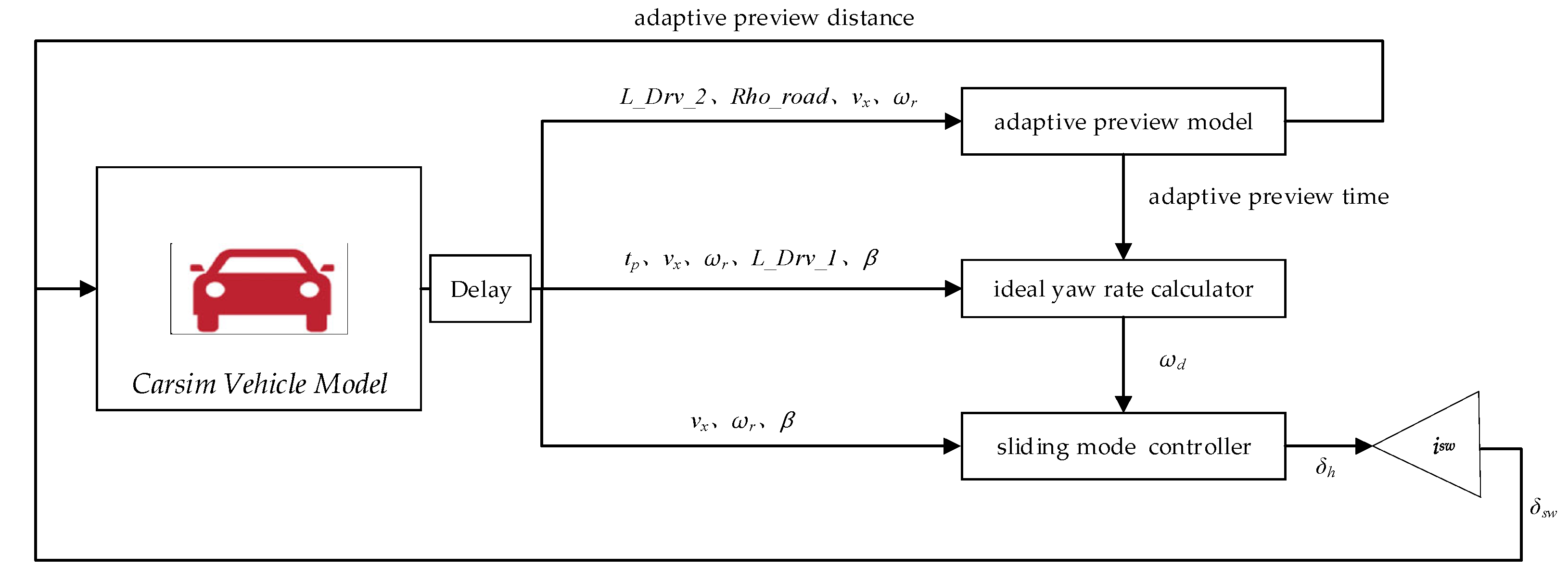
5.1. Construction of Joint Simulation Platform

The vehicle data in Carsim is sent to the model built by Simulink in the form of S-function, the sampling period used in the simulation tests is 0.001 s, and the designed sliding mode controller is added to the model as follows in Figure 9:

Set the input and output parameters of Carsim, the first two are input and the others are output parameters, as follows in

Table 2. Carsim import/export channels.

Parameters	Import/Export Channels	Unit
Lead distance to drive model path	IMP_LX_SEN_1	m
Steering wheel angle	IMP_STEER_SW	deg
Lateral distance to target preview point 2	L_Drv_2	m
Longitudinal speed	Vx_SM	km/h
Yaw rate of vehicle	AV_Y	deg/s
Slip angle of vehicle	Beta	deg
Lateral distance to target preview point 1	L_Drv_1	m

:

The

Table 3. Parameters of vehicle.

Parameters	Value	Unit
m	1820	kg
Iz	1523	kg·m−2
Cf	108,861	N·rad−1
Cr	108,861	N·rad−1
isw	19.562	-

to summarize the parameters of the vehicle used in simulation tests is shown as follows:

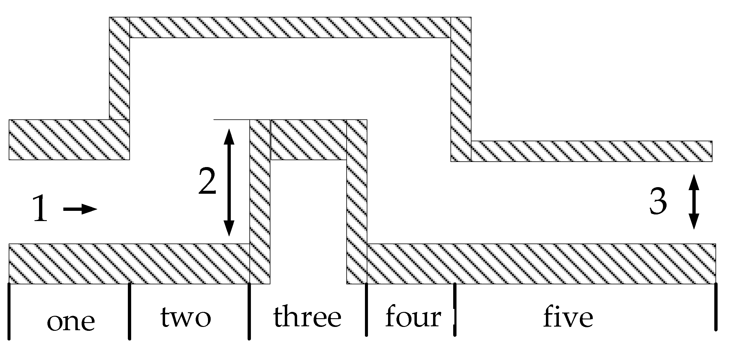
5.2. Double Shift Road Path Planning

Using the ISO/3888-1:2016 standard double shift line with the road centerline as the ideal path, the test route is schematically shown as follows:

The numbers 1 and 2 indicate the direction of travel of the vehicle and the offset of the road, the number 3 indicates the width of the road, and one to five indicate the name of the road section in Figure 10.

Set up the double-shifted road in Carsim in the form of discrete points, and the road centerline coordinate points are set up as shown in

Table 4. Double-shift line road centerline discrete point table.

X (m)	Y (m)	Station (m)	X (m)	Y (m)	Station (m)
0	0	0	95	3.4	90.291
65	0	65	120	3.4	95.292
70	0.1	70.001	125	3.3	125.296
75	0.7	75.037	130	2.4	130.377
80	1.8	80.156	135	1.1	135.543
85	2.8	85.255	140	0.2	145.627
90	3.4	90.291	200	0	200.627

:

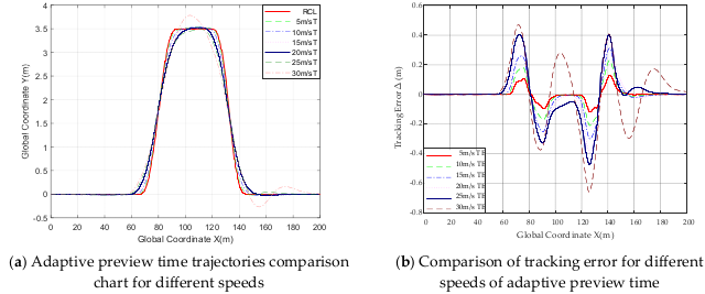
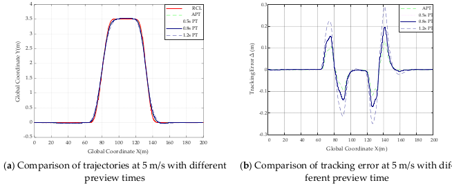
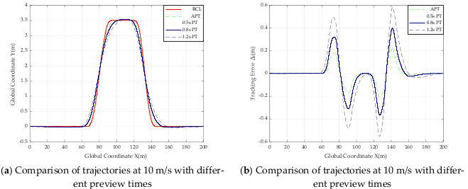
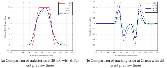
5.3. Simulation Verification of Double-Shifted Line Working Condition

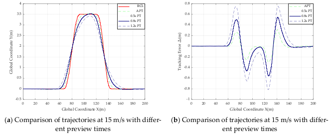
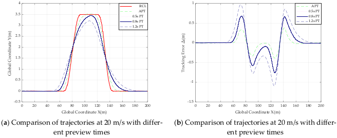
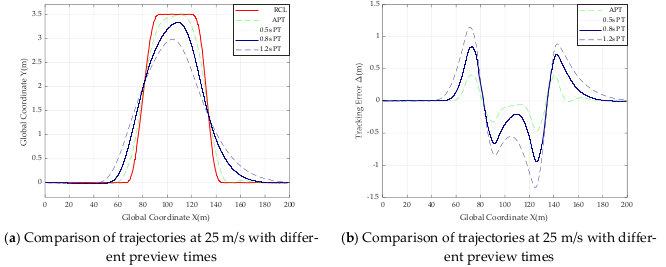
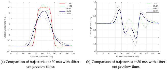
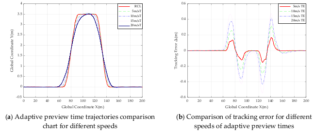
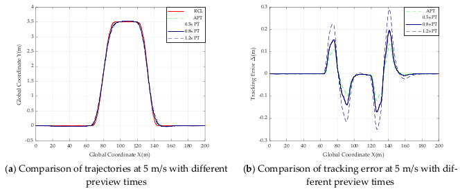
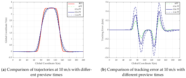
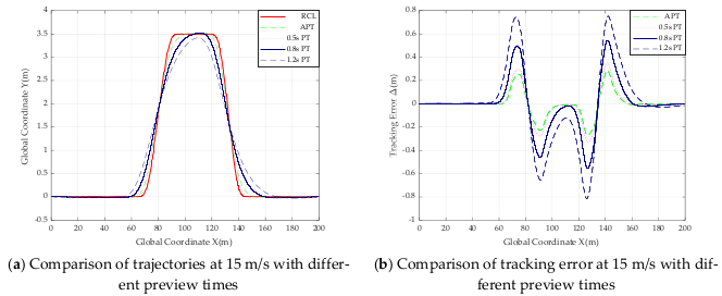
5.3.1. Double-Shifted Working Condition under High Adhesion Coefficient Pavement

Set the road surface coefficient as μ = 0.9, and let the vehicle track the set double-shift line path at longitudinal speed of 5 m/s, 10 m/s, 15 m/s, 20 m/s, 25 m/s and 30 m/s, respectively. Taking the vehicle mass center to road centerline offset as the tracking error, the combined simulation results are as follows (where RCL is road center line, T is trajectory, TE is tracking error, APT is adaptive preview time, PT is preview time):

As can be seen from Figure 11, the tracking accuracy at Section 1 and Section 5 basically remains within 0.025 m, and as the speed increases from 5 m/s to 20 m/s (i.e., from 18 km/h to 72 km/h), the error at Section 5 increases to 0.05 m at 25 m/s, which is still within the acceptable range. However, the result is not within the acceptable range at 30 m/s, the trajectory is unsatisfactory and the tracking error of 0.27 m is too high for tracking.

The analysis of Section 2 and Section 4 is neglected because the reference is the centerline of the road at the location at that time. The differences between the peak point of the trajectory and the road centerline at each of the three locations on the road section at different speeds are 0.0307 m, 0.0296 m, 0.0294 m, 0.0242 m, −0.0154 m, 0.2825 m (from 5 m/s to 30 m/s, at 5 m/s intervals); the differences between the point at Global Coordinate X = 95 m and the road centerline at different speeds are −0.0186 m, −0.0470 m, −0.0942 m, −0.1491 m, −0.1757 m and −0.018 m; the differences between the point at Global Coordinate X = 120 m and the road centerline at different speeds are −0.0047 m, −0.0307 m, −0.0789 m, −0.1570 m, −0.2517 m and −0.4226 m (from 5 m/s to 30 m/s). From these data above, as the speed of the vehicle continues to increase, the maximum error in Section 3 increases and the tracking effect of the controller gradually diminishes. It can be seen that at speeds of 5–25 m/s, the maximum offset from the road centerline on Section 3 does not exceed 0.26 m; thus, the tracking effect of the sliding mode controller based on adaptive preview time is good.

Table 5. Maximum and minimum offsets for different preview time and different speed for road segment three.

Speed (m/s)	Adaptive Preview Time (m)		0.5 s Preview Time (m)		0.8 s Preview Time (m)		1.2 s Preview Time (m)
	Maximum Offset	Minimum Offset	Maximum Offset	Minimum Offset	Maximum Offset	Minimum Offset	Maximum Offset	Minimum Offset
5	0.0307	−0.0186	0.0307	−0.0191	0.0302	−0.0298	0.0354	−0.0570
10	0.0296	−0.0470	0.0296	−0.0309	0.0350	−0.1281	0.0310	−0.2718
15	0.0294	−0.0942	0.0278	−0.1182	0.0170	−0.2640	−0.0815	−0.4975
20	0.0242	−0.1570	0.0152	−0.2028	−0.0540	−0.4232	−0.2942	−0.8555
25	−0.0154	−0.2517	−0.0172	−0.2769	−0.1719	−0.6516	−0.5247	−1.1763
30	0.2825	−0.4226	−0.0937	−0.4095	−0.3068	−0.8712	−0.7394	−1.4423

is made of data from Figure 12, Figure 13, Figure 14, Figure 15, Figure 16 and Figure 17, and it is clarified that the maximum offset and the minimum offset are taken as the difference between the highest point and the two endpoints on the road Section 3 and the centerline of the road:

From Table 5 and all the trajectory comparison graphs above, the absolute value of the maximum offset in road Section 3 from 5 m/s to 25 m/s does not exceed 0.031 m, and the absolute value of the minimum offset does not exceed 0.260 m, so the controller can be judged to be tracking well at speeds from 5 m/s to 20 m/s. The smaller absolute value of the error of the designed SMC controller based on adaptive preview time compared to other controllers with fixed preview times of 0.5 s, 0.8 s and 1.2 s, the results of these data prove that the effectiveness of the designed controller when road adhesion coefficient is 0.9.

5.3.2. Double-Shifted Working Condition under Low Adhesion Coefficient Pavement

Set the road adhesion coefficient as μ = 0.5, and let the vehicle track the set double-shift line path with longitudinal speed of 5 m/s, 10 m/s, 15 m/s and 20 m/s respectively. Taking the vehicle mass center to road centerline offset as the tracking error, the joint simulation results are as follows (where RCL is road center line, T is trajectory, TE is tracking error, APT is adaptive preview time, PT is preview time).

From Figure 18 it can be seen that when the speed is set between the range of 5 m/s to 20 m/s, the tracking accuracy of road Section 1 and the road Section 5 basically remain within 0.037 m; this shows that the designed controller tracks well on sections on and five from 5 m/s to 20 m/s.

The analysis of Section 2 and Section 4 is neglected because the reference is the centerline of the road at the location at that time. The differences between the peak point of the trajectory and the road centerline at each of the three locations on the road section at different speeds are 0.0313 m, 0.0289 m, 0.0265 m and 0.0312 m (from 5 m/s to 20 m/s, at 5 m/s intervals); the differences between the point at Global Coordinate X = 95 m and the road centerline at different speeds are −0.0124 m, −0.0481 m, −0.0864 m and −0.1679 m; and the differences between the point at Global Coordinate X = 120 m and the road centerline at different speeds are −0.0017 m, −0.0254 m, −0.0435 m and −0.1639 m. From these data above, as the speed of the vehicle continues to increase, the maximum offset and the minimum offset in Section 3 increases and the tracking effect of the controller gradually diminishes. It can be seen that at speeds of 5–20 m/s, the maximum offset from the road centerline on Section 3 does not exceed 0.0320 m and the minimum offset from the road centerline on Section 3 does not exceed 0.1680 m. This shows that the tracking effect of the sliding mode controller based on adaptive preview time is good when road adhesion coefficient is 0.5.

Table 6. Maximum offsets and minimum offsets for different preview times and different speeds for road segment three.

Speed (m/s)	Adaptive Preview Time (m)		0.5 s Preview Time (m)		0.8 s Preview Time (m)		1.2 s Preview Time (m)
	Maximum Offset	Minimum Offset	Maximum Offset	Minimum Offset	Maximum Offset	Minimum Offset	Maximum Offset	Minimum Offset
5	0.0307	−0.0186	0.0307	−0.0191	0.0302	−0.0298	0.0354	−0.0570
10	0.0296	−0.0470	0.0296	−0.0309	0.0350	−0.1281	0.0310	−0.2718
15	0.0294	−0.0942	0.0278	−0.1182	0.0170	−0.2640	−0.0815	−0.4975
20	0.0242	−0.1570	0.0152	−0.2028	−0.0540	−0.4232	−0.2942	−0.8555

is made of data from Figure 19, Figure 20, Figure 21 and Figure 22, and it is clarified that the maximum offset and the minimum offset is taken as the difference between the highest point and the two endpoints on the road Section 3 and the centerline of the road:

From Table 6 and the above trajectory comparison graph, it can be seen that the absolute value of the maximum offset in road Section 3 from 5 m/s to 20 m/s does not exceed 0.031 m, and the absolute value of the minimum offset does not exceed 0.1600 m, so the controller can be judged to be tracking well at speeds from 5 m/s to 20 m/s. The smaller absolute value of the error of the designed SMC controller based on adaptive preview time compared to other controllers with fixed preview times of 0.5 s, 0.8 s and 1.2 s, the results of these data prove the effectiveness of the designed controller when the road adhesion coefficient is 0.5.

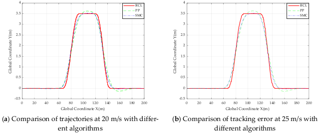
5.3.3. Comparative Simulation Experiments with Another Typical Algorithm

PP (Pure Pursuit) is a typical and transversal algorithm; it is a geometric algorithm based on a single preview point, with good robustness to the outside world, essentially referring to a fixed preview distance algorithm. Its structure is shown in the following diagram in Figure 23.

In ΔOAB, we can know:

$$\angle \mathrm{AOC}=2\angle \mathrm{CAB}=2\mathit{\alpha }$$

(36)

From the sine theorem, we know that:

$$\frac{{\mathit{l}}_{\mathit{d}}}{\mathit{sin}2\mathit{\alpha }}=\frac{\mathit{R}}{\mathit{sin}\left(\frac{\mathit{\pi }}{2}-\mathit{\alpha }\right)}$$

(37)

From the Ackermann turn, it follows that:

$$\mathit{R}=\frac{{\mathit{l}}_{\mathit{d}}}{2\mathit{sin}\mathit{\alpha }}$$

(38)

Join Equations (37) and (38), we can know:

$$\mathit{\delta }\left(\mathit{t}\right)=\mathit{arctan}(\frac{2\mathit{Lsin}\left(\mathit{\alpha }\right(\mathit{t})\mathrm{)}}{{\mathit{l}}_{\mathit{d}}})$$

(39)

Comparison tests with a road adhesion coefficient of 0.9 and vehicle speeds of 15 m/s and 20 m/s with double shift conditions, the contrasted figures of the simulation results are shown below:

From simulation results of Figure 24, the errors of the two algorithms on Section 1 is less than 0.01 m and less than 0.015 m, so the PP algorithm tracks better in this part. Meanwhile, on Section 3, the peak point of the trajectory of the PP algorithm is larger than that of the SMC algorithm, so the SMC algorithm tracks better in this part. On Section 5, the tracking error of the PP algorithm is less 0.15 m and the SMC algorithm tracking five rubbing sweat is less than 0.025 m, so the SMC algorithm tracking effect is better in this part. Overall, the trajectory of the SMC algorithm follows the road centerline more closely than the trajectory of the PP algorithm, compared with fixed preview distance in the PP algorithm, the tracking effect of the sliding mode controller based on adaptive preview time is better.

6. Conclusions

The validity of the model established by Simulink–Carsim joint simulation is verified by the simulation results, and the results show that the adaptive optimization function of the preview time is established, and the optimization index is established based on the trajectory deviation, boundary distance, and vehicle steering motion characteristics to realize the adaptive change of the preview time of the sliding mode controller. In order to solve the problem of jitter in the sliding mode control, a low-pass filter has been added, and from the results, the jitter of the control volume is greatly reduced after the low-pass filter.

The results of the simulation show that the designed controller tracks well at a coefficient of adhesion of 0.9 and at speeds between 0 and 25 m/s, also tracking well at a coefficient of adhesion of 0.5 and at speeds between 0 and 20 m/s, and compared with the fixed preview time controller (PP), it can better reflect the driver’s operating characteristics, the boundary constraints, the motion response characteristics of the whole vehicle, and has a better path tracking effect. The controller has a better control effect and verifies the effectiveness and adaptability of the controller to speed and adhesion coefficient. This demonstrates the designed controller’s ability to adapt to both high and low adhesion surfaces, but as the adhesion coefficient decreases, the maximum speed that can be achieved without reducing tracking accuracy gradually decreases. The selection of preview time is very important for the input of the controller, so there is too much reliance on the right preview time. Furthermore, the question of jitter is difficult to eliminate completely, so there are some problems for practical control.

This study only considers low-pass filter in combination with sliding mode controller, and does not consider complex filters such as Kalman filter, and the design of sliding mode surface in subsequent studies can consider the higher-order sliding mode theory.

References

1. Cai, G.; Liu, H.; Feng, J.; Xu, L.; Yin, G. Review on the research of motion planning and control for intelligent vehicles. J. Automot. Saf. Energy 2021, 12, 279–297. [Google Scholar]
2. Xu, Y.; Tang, W.; Chen, B.; Qiu, L.; Yang, R. A Model Predictive Control with Preview-Follower Theory Algorithm for Trajectory Tracking Control in Autonomous Vehicles. Symmetry 2021, 13, 381. [Google Scholar] [CrossRef]
3. Li, Z.; Wang, P.; Liu, H.; Hu, Y.; Chen, H. Coordinated Longitudinal and Lateral Vehicle Stability Control Based on the Combined-Slip Tire Model in the MPC Framework. Mech. Syst. Signal Process. 2021, 161, 107947. [Google Scholar] [CrossRef]
4. Loof, J.; Besselink, I.; Nijmeijer, H. Automated Lane Changing with a Controlled Steering-Wheel Feedback Torque for Low Lateral Acceleration Purposes. IEEE Trans. Intell. Veh. 2019, 4, 578–587. [Google Scholar] [CrossRef]
5. Yang, T.; Bai, Z.; Li, Z.; Feng, N.; Chen, L. Intelligent Vehicle Lateral Control Method Based on Feedforward+ Predictive LQR Algorithm. Actuators 2021, 10, 228. [Google Scholar] [CrossRef]
6. Rao, L.G.; Narayanan, S. Optimal Response of Half Car Vehicle Model with Sky-Hook Damper Based on LQR Control. Int. J. Dyn. Control. 2020, 8, 488–496. [Google Scholar]
7. Hang, P.; Xia, X.; Chen, X. Handling Stability Advancement With 4WS and DYC Coordinated Control: A Gain-Scheduled Robust Control Approach. IEEE Trans. Veh. Technol. 2021, 70, 3164–3174. [Google Scholar] [CrossRef]
8. Zhang, S.; Zhao, X.; Zhu, G.; Shi, P.; Hao, Y.; Kong, L. Adaptive Trajectory Tracking Control Strategy of Intelligent Vehicle. Int. J. Distrib. Sens. Netw. 2020, 16, 155014772091698. [Google Scholar] [CrossRef]
9. Wu, H.; Si, Z.; Li, Z. Trajectory Tracking Control for Four-Wheel Independent Drive Intelligent Vehicle Based on Model Predictive Control. IEEE Access 2020, 8, 73071–73081. [Google Scholar] [CrossRef]
10. Shen, C.; Shi, Y. Distributed Implementation of Nonlinear Model Predictive Control for AUV Trajectory Tracking. Automatica 2020, 115, 108863. [Google Scholar] [CrossRef]
11. Zhang, Y.; Xia, Y.; Cheng, H.; Huang, L.; Zhao, F.; Lv, L. Research on Lateral Control of Intelligent Vehicle Path Tracking. J. Chongqing Inst. Technol. 2021, 35, 53–61. [Google Scholar]
12. Hu, J.; Xiong, S.; Zha, J.; Fu, C. Lane Detection and Trajectory Tracking Control of Autonomous Vehicle Based on Model Predictive Control. Int. J. Automot. Technol. 2020, 21, 285–295. [Google Scholar] [CrossRef]
13. Alika, R.; Mellouli, E.M.; Tissir, E.H. Optimization of Higher-Order Sliding Mode Control Parameter Using Particle Swarm Optimization for Lateral Dynamics of Autonomous Vehicles. In Proceedings of the 2020 1st International Conference on Innovative Research in Applied Science, Engineering and Technology (IRASET), Meknes, Morocco, 16–19 April 2020; IEEE: Piscataway, NJ, USA, 2020; pp. 1–6. [Google Scholar]
14. Liu, W.; Wang, R.; Xie, C.; Ye, Q. Investigation on Adaptive Preview Distance Path Tracking Control with Directional Error Compensation. Proc. Inst. Mech. Eng. Part I J. Syst. Control. Eng. 2020, 234, 484–500. [Google Scholar] [CrossRef]
15. Zhang, J.; Zhou, S.; Shi, Z.; Zhao, J.; Zhu, B. Path planning and tracking control for corner overtaking of driverless vehicle using sliding mode technique with conditional integrators. Control. Theory Appl. 2021, 38, 197–205. [Google Scholar]
16. Zhang, P.; Yang, Z.; Zhao, X.; Yao, L.; Zhang, S. Backward Path Tracking for Tractor-Semitrailer System Based on Sliding Model Control. Agric. Eng. 2021, 11, 103–107. [Google Scholar]
17. Hui, Y. Research on Neural-Network Adaptive Sliding Mode Control of Longitudinal Dynamic Behavior of Intelligent Vehicle. Master Thesis, Jiangsu University, Zhenjiang, China, 2020. [Google Scholar]
18. Du, H.; Man, Z.; Zheng, J.; Cricenti, A.; Zhao, Y.; Xu, Z.; Wang, H. Robust Control for Vehicle Lane-Keeping with Sliding Mode. In Proceedings of the 2017 11th Asian Control Conference (ASCC), Gold Coast, Australia, 17–20 December 2017; IEEE: Piscataway, NJ, USA, 2017; pp. 84–89. [Google Scholar]
19. Lin, F.; Sun, M.; Wu, J.; Qian, C. Path Tracking Control of Autonomous Vehicle Based on Nonlinear Tire Model. Actuators 2021, 10, 242. [Google Scholar] [CrossRef]
20. Chen, W.; Tan, D.; Wang, H.; Wang, J.; Xia, G. A class of driver directional control model based on trajectory prediction. J. Mech. Eng. 2016, 52, 106–115. [Google Scholar] [CrossRef]
21. Jin, X.; Zhang, J.; Liu, Y.; Wang, Q. Research on adaptive optimal preview model based on Stanley algorithm. Comput. Eng. 2018, 44, 42–46. [Google Scholar]
22. Li, H. Optimal Preview Control Driver Model with Adaptive Preview Time. JME 2010, 46, 106. [Google Scholar] [CrossRef]
23. Li, X.; Zhang, X.; Li, Z.; Cai, J.; Fu, Y. Sliding Mode Control for Digital Hydraulic Cylinder Servo Systems Based on Low Pass Filter. Chin. Hydraul. Pneum. 2014, 12, 72–74. [Google Scholar]
24. Zhao, L.; Wang, S.; Wang, H. LDF-based sliding mode control for robots. Comput. Eng. Appl. 2009, 45, 236–238. [Google Scholar]
Figure 1. Vehicle two-degree-of-freedom dynamics model.
Actuators 11 00034 g001
Figure 2. Steady-state transverse pendulum angle single-point preview model.
Actuators 11 00034 g002
Figure 3. Controller design diagram.
Actuators 11 00034 g003
Figure 4. Sliding mode control systems based on low-pass filters.
Actuators 11 00034 g004
Figure 5. The steering wheel angle with and without filtering at RAC = 0.9 and VS = 10 m/s.
Actuators 11 00034 g005
Figure 6. The steering wheel angle with and without filtering at RAC = 0.9 and VS = 20 m/s.
Actuators 11 00034 g006
Figure 7. The steering wheel angle with and without filtering at RAC = 0.5 and VS = 10 m/s.
Actuators 11 00034 g007
Figure 8. The steering wheel angle with and without filtering at RAC = 0.5 and VS = 20 m/s.
Actuators 11 00034 g008
Figure 9. CarsimSimulink Joint Simulation Model.
Actuators 11 00034 g009
Figure 10. Double-shift line test road diagram.
Actuators 11 00034 g010
Figure 11. Comparison of trajectories and tracking error for different speeds of adaptive preview time.
Actuators 11 00034 g011
Figure 12. Comparison of trajectories and tracking error with different preview times at 5 m/s.
Actuators 11 00034 g012
Figure 13. Comparison of trajectories and tracking error with different preview times at 10 m/s.
Actuators 11 00034 g013
Figure 14. Comparison of trajectories and tracking error with different preview times at 15 m/s.
Actuators 11 00034 g014
Figure 15. Comparison of trajectories and tracking error with different preview times at 20 m/s.
Actuators 11 00034 g015
Figure 16. Comparison of trajectories and tracking error with different preview times at 25 m/s.
Actuators 11 00034 g016
Figure 17. Comparison of trajectories and tracking error with different preview times at 30 m/s.
Actuators 11 00034 g017
Figure 18. Comparison of trajectories and tracking error for different speeds of adaptive preview time.
Actuators 11 00034 g018
Figure 19. Comparison of trajectories and tracking error with different preview times at 5 m/s.
Actuators 11 00034 g019
Figure 20. Comparison of trajectories and tracking error with different preview times at 10 m/s.
Actuators 11 00034 g020
Figure 21. Comparison of trajectories and tracking error with different preview times at 15 m/s.
Actuators 11 00034 g021
Figure 22. Comparison of trajectories and tracking error with different preview times at 20 m/s.
Actuators 11 00034 g022
Figure 23. Structural diagram of the PP algorithm, where δ is front wheel steering angle; L is wheelbase of vehicle; ld is preview distance; draw the circle using the preview distance as the chord length of the circle, and R is the radius of the circle; the circle intersects the trajectory at point C; α is the angle of the chord to the vehicle body.
Actuators 11 00034 g023
Figure 24. Comparison experiments between PP and SMC algorithms at different speeds.
Actuators 11 00034 g024