A Precise Stabilization Method for Linear Stochastic Time-Delay Systems

Abstract

Based on ensuring the steady-state performance of the system, some dynamic performance indicators that have not yet been realized in linear stochastic systems with time-delay are discussed in this paper. First, in view of the relationship between system eigenvalues and system performances, the region stability is provided, which can reflect the dynamic performance of the systems. Second, the design scheme of the region stabilization controller is given based on the region stability, so that the closed-loop system has the corresponding dynamic performance. Third, this paper also designs an algorithm to deal with the situation in which the eigenvalues are located in the non-connected region in order to obtain more accurate control system dynamic performance. Finally, an example shows how the precise control method dominates the dynamic performance of the system.

1. Introduction

Linear stochastic time-delay systems (LSTDSs) have always been the focus of research in the field of control, and various subfields have also been developed. The time-delay and stochastic terms are usually the important reasons for system instability or poor performance. Due to their complexity and comprehensive application fields, LSTDSs have become very active and have developed in various areas based on different focuses, such as stability analysis and stabilization [1,2,3], control system synthesis [4,5,6], uncertain system control [7,8,9], filter design [10,11,12], etc.

Regardless of the branch of LSTDSs, stability is the most vital element for the development of LSTDSs. Up to now, almost all stability analyses for LSTDSs can only provide asymptotically stable conditions, that is the state of the system approaches zero as time tends to infinity. These methods often fail to help us regulate dynamic performance indicators of the system. In practical engineering, the system is often required to have certain dynamic performance. For example, some systems do not allow oscillating responses; some systems wish to have moderate damping; some systems wish to have a faster response speed.

As is well known, there are pole assignment and regional pole assignment of the linear time-invariant systems, which can control the dynamic performance of the system very well. The dynamic performances of the system are strongly linked with the distribution position of the system eigenvalues. As a generalization of the pole allocation method, spectrum criteria have made great progress in recent years. A robust regional pole placement was investigated in [13]. By the spectrum technique, interval stability and stabilization of the stochastic systems (LSSs) were explored in [14,15,16,17]. The Pth moment region stability/stabilization and some related control questions for LSSs were addressed in [18,19,20].

Although the research on region stability and stabilization has made great progress, it is not easy to generalize these conclusions to LSTDSs because of the influence of time-delay terms and stochastic terms. There are currently no results on the regionally stable conditions of LSTDSs, nor the design of region controllers, as far as we know. Based on the previous discussion, this paper proposes the regional stability conditions and controller design, which can reflect the system stability characteristics in more detail and regulate the dynamic performance of the closed-loop system. The main innovations of this paper are as follows:

First, a new region stability for LSTDSs is given based on the properties of LSTDSs, which describes more accurate system performance.

Second, important region stability criteria of LSTDSs are presented by LMIs, which are convenient to calculate. As a finer partition, the stability criteria for unconnected regions are also investigated by an algorithm. The criteria can be thought of as a generalization of the existing stability criteria for LSTDSs.

Third, the region stabilization method of LSTDSs is addressed. Using this new method, different controllers can be designed according to the actual system’s requirements for performance indicators. There is no relevant conclusion that can achieve this as far as we know.

The main body of this paper consists of seven parts. The description of the system, the definition of region stability/stabilization, and some lemmas are presented in Section 2. Section 3 presents the sufficient conditions for the region stability of LSTDSs. Section 4 discusses the region stabilization controllers of LSTDSs. An unconnected region stabilization algorithm and a pole assignment algorithm for LSTDSs are presented in Section 5. Section 6 provides an example to illustrate the advantages of region stabilization. A summary of the main points is given in Section 7.

Notation:$\parallel ·\parallel$: two-norm. $tr\left(A\right)$: the sum of the principal diagonals of matrix A. $det\left(A\right)$: the determinant of matrix A. $\Im \left(\lambda \right)$: the imaginary part of the complex number $\lambda$. $\Re \left(\lambda \right)$: the real part of the complex number $\lambda$. $\mathcal{E}(·)$: mathematical expectation operator. $\sigma \left(A\right)$: the spectrum set of A.

2. Preliminaries

Consider

$$\left\{\begin{array}{cc}\hfill dx\left(t\right)& =[Ax\left(t\right)+A_{d}x(t-\nu \left(t\right))+C_1{u}_1\left(t\right)]dt\hfill \\ & +[Bx\left(t\right)+B_{d}x(t-\nu \left(t\right))+C_2{u}_2\left(t\right)]dw\left(t\right),\hfill \\ & :=\phi \left(x\right(t),t)dt+\psi \left(x\right(t),t)dw\left(t\right),\hfill \\ \hfill x\left(t\right)& =\rho \left(t\right),t\in [-l,0]\hfill \end{array}\right.$$

(1)

where $d·$ is the differential symbol, $x\left(t\right)\in {\mathcal{R}}^n$ is a state vector, and $w\left(t\right)$ is an independent stochastic variable, a standard one-dimensional Wiener process. $\rho \left(t\right)$ is the initial condition in $L_{F_0}^2([-l,0];{\mathcal{R}}^n).$$\tau \left(t\right)$ satisfies

$$0\le \nu \left(t\right)\le l,\dot{\nu }\left(t\right)\le \mu ,$$

(2)

where $\mu$ and l are known. $A,A_d,B,B_d,C_1$, and $C_2$ are given matrices,

$$\begin{array}{ccc}\hfill u_1\left(t\right)& =& K_{A}x\left(t\right)+K_{A_d}x(t-\tau \left(t\right)),\hfill \end{array}$$

(3)

$$\begin{array}{ccc}\hfill u_2\left(t\right)& =& K_{B}x\left(t\right)+K_{B_d}x(t-\tau \left(t\right)).\hfill \end{array}$$

(4)

The special case of the system (1),

$$\left\{\begin{array}{cc}\hfill \dot{x}\left(t\right)& =Ax\left(t\right),\hfill \\ \hfill x\left(0\right)& =x_0,\hfill \end{array}\right.$$

(5)

is very instructive for the control strategy of the system, although it is very simple.

We first investigate the system (5) and present sufficient conditions for its region stability. Then, according to the region stability conditions of System (5), the control strategy and controller design of System (1) are addressed.

Definition 1.

System (5) has region $(-b,-a)\times (c,d)$ and $(-b,-a)\times (-d,-c)$ stability, if System (5) is stable and

$$\Re \left[\sigma \right(A\left)\right]\in (-b,-a),|\Im [\sigma \left(A\right)\left]\right|\in (c,d).$$

As a particular case of Definition 1, the definition of interval stability is shown below.

Definition 2.

System (5) has interval $(-b,-a)$ stability, if

$$\Re \left[\sigma \right(A\left)\right]\in (-b,-a),$$

and System (5) is stable.

Definition 3.

([1]). The LSTDS (1) is asymptotically stable, if, for arbitrary initial state $x_0$,

$$\underset{t\to \infty }{lim}\mathcal{E}{\parallel x(t,t_0)\parallel }^2=0$$

can be obtained.

Definition 4.

The LSTDS (1) has region $(-b,-a)\times (c,d)$ and $(-b,-a)\times (-d,-c)$ stabilization, if

$$\begin{array}{ccc}& & \underset{t\to \infty }{lim}\mathcal{E}{\parallel x(t,t_0)\parallel }^2=0,\hfill \end{array}$$

(6)

$$\begin{array}{ccc}& & Re\left[\sigma (A+C_1{K}_A)\right]\in (-b,-a),\hfill \end{array}$$

(7)

$$\begin{array}{ccc}& & |Im\left[\sigma (A+C_1{K}_A)\right]|\in (c,d),\hfill \end{array}$$

(8)

$$\begin{array}{ccc}& & {(A_d+C_1{K}_{A_d})}^T(A_d+C_1{K}_{A_d})<ϵI,\hfill \end{array}$$

(9)

$$\begin{array}{ccc}& & {(B+C_2{K}_B)}^T(B+C_2{K}_B)<ϵI,\hfill \end{array}$$

(10)

$$\begin{array}{ccc}& & {(B_d+C_2{K}_{B_d})}^T(B_d+C_2{K}_{B_d})<ϵI,\hfill \end{array}$$

(11)

where ϵ is a very small positive number.

Remark 1.

Compared with the mean square stability, the region stability condition can describe the dynamic and steady-state performance of the system more accurately, rather than just judging its stability. Of course, the judgment conditions of regional stability are also more complex. Conditions (9)–(11) reduce the effects of the time-delay term and the stochastic term in the system (1) to a negligible degree by designing the controller. Then, according to Definition 1, we can restrict the eigenvalues to the corresponding regions by adding the controller to the rest of the system. In short, we simplified System (1) to System (5) by adding controllers and then carried out region stability control for System (5).

Lemma 1.

([20]). For any positive definite matrix $Q\in {\mathcal{R}}^{n\times n}$ and any $P\in {\mathcal{R}}^{n\times n}$, then

$$-P^T{Q}^{-1}P\le Q-P-P^T.$$

3. Region Stability

In this section, the sufficient conditions for System (5)’s region stability are presented. Meanwhile, a sufficient and necessary condition for the interval stability is presented.

Theorem 1.

The linear system (5) has asymptotically rectangle region $(-b,-a)\times (c,d)$ and $(-b,-a)\times (-d,-c)$ stability, that is $|\Im [\sigma \left(A\right)\left]\right|\in (c,d)$ and $\Re \left[\sigma \right(A\left)\right]\in (-b,-a)$, if the following LMI:

$${(A+aI)}^{T}P+P(A+aI)<0,$$

(12)

$${(-A-bI)}^{T}P+P(-A-bI)<0$$

(13)

has a solution $P>0$, and

$$(c^2+\frac{{(a-b)}^2}{4})I<{(A+\frac{a+b}{2}I)}^T(A+\frac{a+b}{2}I)<d^{2}I,$$

(14)

where $0\le a<b$ and $0\le c<d$.

Proof. 

First, let us prove $Re\left[\sigma \right(A\left)\right]\in (-b,-a)$, if and only if (12) and (13) hold. $Re\left[\sigma \right(A\left)\right]\in (-b,-a)$ iff the next two systems are stable. That is to say,

$$\left\{\begin{array}{cc}\hfill \dot{x}\left(t\right)& =(A+aI)x\left(t\right),\hfill \\ \hfill x\left(0\right)& =x_0,\hfill \end{array}\right.$$

(15)

and

$$\left\{\begin{array}{cc}\hfill \dot{x}\left(t\right)& =-(A+bI)x\left(t\right)\hfill \\ \hfill x\left(0\right)& =x_0,\hfill \end{array}\right.$$

(16)

are asymptotic stability. According to the Lyapunov stability criteria, the interval has $(-b,-a)$ stability if and only if (12) and (13) hold.

Secondly, assuming $\sigma \left(A\right)={\alpha }_k+{\beta }_{k}i(k=1,\cdots ,n)$, then

$$\sigma [(A+\frac{a+b}{2}I){(A+\frac{a+b}{2}I)}^T]={({\alpha }_k+\frac{a+b}{2})}^2+{\beta }_k^2.$$

Due to $Re\left[\sigma \right(A\left)\right]\in (-b,-a)$, i.e., $-b<{\alpha }_k<-a,$ such that

$${\beta }_k^2<{({\alpha }_k+\frac{a+b}{2})}^2+{\beta }_k^2<{(\frac{a-b}{2})}^2+{\beta }_k^2.$$

On the basis of (14), we have

$$c^2<{\beta }_k^2.$$

${\beta }_k^2<d^2$ can be obtained in parallel. According to the above two inequalities, $\left|Im\right[\sigma \left(A\right)\left]\right|\in (c,d)$ can be obtained. Finally, the satisfaction of (12–14) ensures that the system (5) has region $(-b,-a)\times (c,d)$ stability. The proof is complete. □

Remark 2.

The asymptotic stability in the sense of Lyapunov can only reflect the steady-state performance of the system, but cannot reflect the dynamic performance of the systems. Based on the relationship between the system poles and system performance indicators, region stability can not only reflect the steady-state performance, but also reflect the dynamic performance of the system. That is to say, regional stability grasps the dynamic performance of the system by examining the pole distribution of the system. Only asymptotic stability with the poles in the left half-plane guarantees that the system is stable.

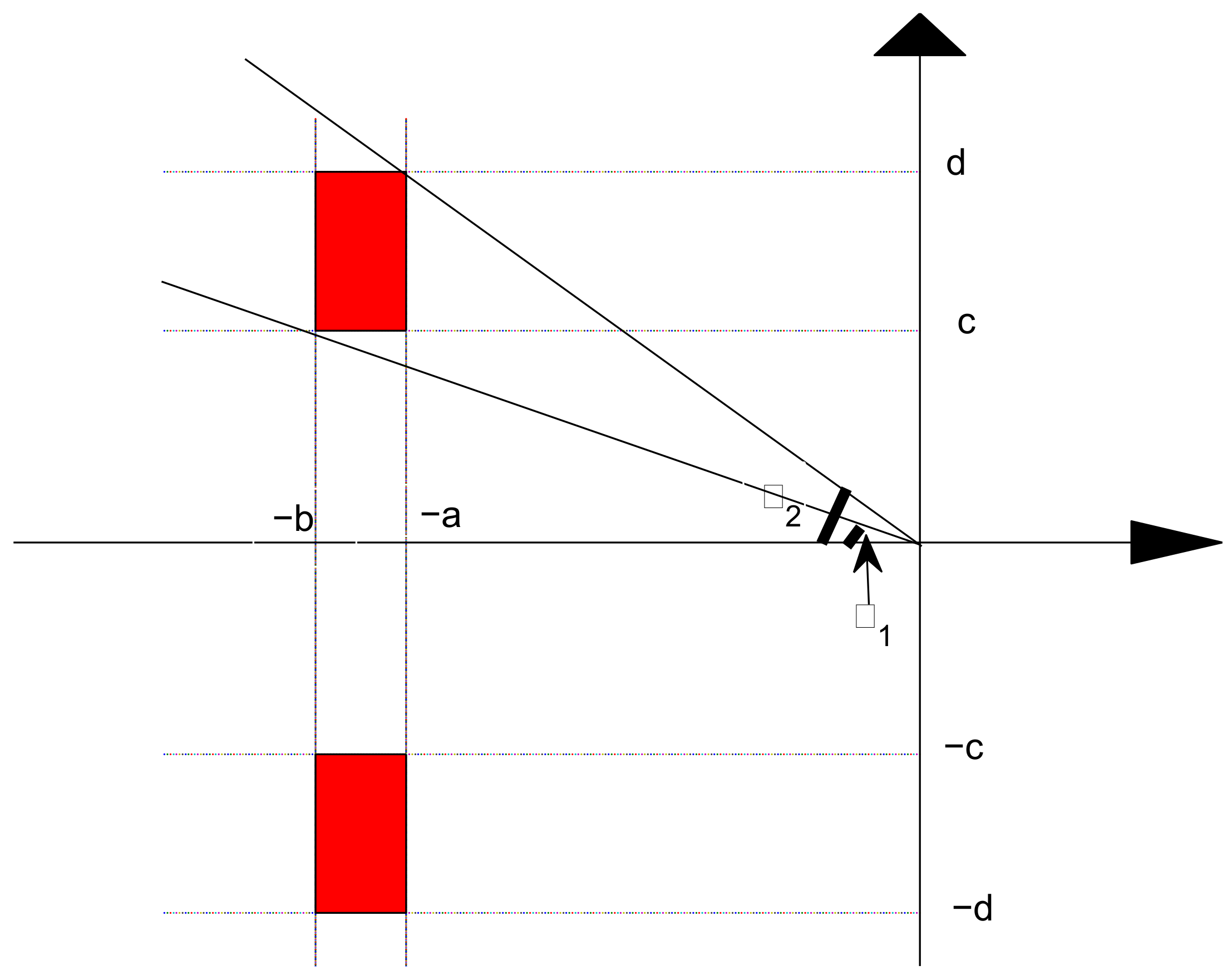
Remark 3.

Most of the current region stability studies focus on convex regions, because convex regions can be easily calculated by means of efficient methods for solving linear matrix inequalities. Theorem 1 gives a disconnected region. It will be more precise to judge the dynamic performance of the system, but it will bring great difficulties to the subsequent controller design. The disconnected region is shown in Figure 1. If $c=0$, then region $(-b,-a)\times (c,d)$ and $(-b,-a)\times (-c,-d)$ turn into a convex region $(-b,-a)\times (-d,d)$.

Remark 4.

In engineering applications, it is usually desirable for the system to have a fast response speed, moderate damping, and a shorter regulation time. As a consequence, the general requirements are generally from 0.4 to 0.8 (see Reference [21] for details). In other words,

$$0.4<arctan{\alpha }_1<arctan{\alpha }_2<0.8$$

as in Figure 1.

As mentioned in Remark 3, the stability analysis and control of non-convex regions are often complicated. For the ease of calculation, we first deal with the case of convex regions. The case of disconnected regions will be discussed in detail in Section 4 by designing the algorithm.

Theorem 2.

The system (5) has region $(-b,-a)\times (-d,d)$ stability, i.e., $\Im \left[\sigma \right(A\left)\right]\in (-d,d)$ and $\Re \left[\sigma \right(A\left)\right]\in (-b,-a)$, if the following LMI:

$${(A+aI)}^{T}P+P(A+aI)<0,$$

(17)

$${(-A-bI)}^{T}P+P(-A-bI)<0$$

(18)

has a solution $P>0$, and

$${(A+\frac{a+b}{2}I)}^T(A+\frac{a+b}{2}I)<d^{2}I,$$

(19)

where $b>a\ge 0$ and $d\in {\mathcal{R}}^{+}$.

When only considering the convergence or divergence of the system and the rate of convergence, a sufficient and necessary condition can be addressed below as a particular case of Theorem 1.

Corollary 1.

System (5) has interval $(-b,-a)$ stability, i.e., $\Re \left[\sigma \right(A\left)\right]\in (-b,-a)$, iff

$${(A+aI)}^{T}P+P(A+aI)<0,$$

$${(-A-bI)}^{T}P+P(-A-bI)<0$$

has a solution $P>0$, where $b>a\ge 0.$

Remark 5.

The stability of the interval can judge the stability of the system, and it can also determine the convergence speed of the system. The farther the interval is from the imaginary axis on the negative half-plane, the faster the system converges. Theorem 1 is transformed into a stable condition in the usual sense as $a=0$ and $b=\infty$.

4. Region Stabilization

Region $(-b,-a)\times (-d,d)$ stabilization of System (1) is investigated in this section, which could dominate the convergence speed of the system states and could adjust the damping ratio to an extent.

Theorem 3.

For given invariants μ, $l>0$, and $ϵ>0$, LSTDS (1) has asymptotic region $(-b,-a)\times (-d,d)$ stabilization; if (2) holds, there are symmetric matrices $\widehat{Q}>0,L>0,\widehat{R}>0$,

$$Y=\left[\begin{array}{ccc}{\widehat{Y}}_{11}& {\widehat{Y}}_{12}& {\widehat{Y}}_{13}\\ *& {\widehat{Y}}_{22}& {\widehat{Y}}_{23}\\ *& *& {\widehat{Y}}_{33}\end{array}\right]\ge 0$$

and arbitrary matrices with appropriate dimensions ${\widehat{N}}_j,{\widehat{M}}_j,{\widehat{T}}_j,{\widehat{S}}_j(j=1,2,3),$ such that

$$\begin{array}{c}\hfill {\Xi }_1=\left[\begin{array}{cc}ϵ(I-2L)& V_2^T{C}_1^T+L{A}_d^T\\ *& -I\end{array}\right]<0,\end{array}$$

(20)

$$\begin{array}{c}\hfill {\Xi }_2=\left[\begin{array}{cc}ϵ(I-2L)& V_3^T{C}_2^T+L{B}^T\\ *& -I\end{array}\right]<0,\end{array}$$

(21)

$$\begin{array}{c}\hfill {\Xi }_3=\left[\begin{array}{cc}ϵ(I-2L)& V_4^T{C}_2^T+L{B}_d^T\\ *& -I\end{array}\right]<0,\end{array}$$

(22)

$$\begin{array}{c}\hfill \widehat{\Delta }=\left[\begin{array}{ccccc}{\widehat{\Delta }}_{11}& {\widehat{\Delta }}_{12}& {\widehat{\Delta }}_{13}& L{B}^T+V_3^T{C}_2^T& h{\widehat{T}}_1^T\\ *& {\widehat{\Delta }}_{22}& {\widehat{\Delta }}_{23}& 0& h{\widehat{T}}_2^T\\ *& *& {\widehat{\Delta }}_{33}& L{B}_d^T+V_4^T{C}_2^T& 0\\ *& *& *& -L& 0\\ *& *& *& *& -h\widehat{R}\end{array}\right]<0,\end{array}$$

(23)

$$\begin{array}{c}\hfill \widehat{\Lambda }=\left[\begin{array}{cccc}{\widehat{Y}}_{11}& {\widehat{Y}}_{12}& {\widehat{Y}}_{13}& {\widehat{S}}_1\\ *& {\widehat{Y}}_{22}& {\widehat{Y}}_{23}& {\widehat{S}}_2\\ *& *& {\widehat{Y}}_{33}& {\widehat{S}}_3\\ *& *& *& 2L-R\end{array}\right]\ge 0,\end{array}$$

(24)

$$\begin{array}{c}\hfill \Theta =-(A+bI)L-C_1{V}_1-L(A+bI)-V_1^T{C}_1^T<0,\end{array}$$

(25)

$$\begin{array}{c}\hfill {\Xi }_4=\left[\begin{array}{cc}I-(AL+C_1{V}_1)& {(b^2+d^2)}^{1/2}L\\ -{(AL+C_1{V}_1)}^T\\ *& -I\end{array}\right]<0,\end{array}$$

(26)

where

$$\begin{array}{ccc}\hfill {\widehat{\Delta }}_{11}& =& \widehat{Q}+{\widehat{T}}_1+{\widehat{T}}_1^T+{\widehat{S}}_1+{\widehat{S}}_1^T+l{\widehat{Y}}_{11},\hfill \\ \hfill {\widehat{\Delta }}_{12}& =& {[(A+aI)L+C{V}_1]}^T-{\widehat{S}}_1+{\widehat{S}}_2+{\widehat{T}}_2^T+l{\widehat{Y}}_{12},\hfill \\ \hfill {\widehat{\Delta }}_{13}& =& {\widehat{T}}_3^T-{\widehat{T}}_1+l{\widehat{Y}}_{13},\hfill \\ \hfill {\widehat{\Delta }}_{22}& =& -{\widehat{S}}_2-{\widehat{S}}_2^T+l{\widehat{Y}}_{22},\hfill \\ \hfill {\widehat{\Delta }}_{23}& =& A_{d}L+C_d{V}_2-{\widehat{T}}_2+l{\widehat{Y}}_{23},\hfill \\ \hfill {\widehat{\Delta }}_{33}& =& -(1-\mu )\widehat{Q}-{\widehat{T}}_3-{\widehat{T}}_3^T+l{\widehat{Y}}_{33}.\hfill \end{array}$$

Moreover, the stabilization controllers are

$$\begin{array}{ccc}\hfill u_1\left(t\right)& =& V_1{L}^{-1}x\left(t\right)+V_2{L}^{-1}x(t-\tau \left(t\right)),\hfill \\ \hfill u_2\left(t\right)& =& V_3{L}^{-1}x\left(t\right)+V_4{L}^{-1}x(t-\tau \left(t\right)).\hfill \end{array}$$

Proof. 

Substituting the controllers $u_1\left(t\right)$ and $u_2\left(t\right)$ into System (1), the closed-loop system below can be obtained.

$$\left\{\begin{array}{cc}\hfill dx\left(t\right)& =[(A+C_1{K}_A)x\left(t\right)+(A_d+C_1{K}_{A_d})x(t-\nu \left(t\right))]dt\hfill \\ & +[(B+C_2{K}_B)x\left(t\right)+(B_d+C_2{K}_{B_d})x(t-\nu \left(t\right))]dw\left(t\right),\hfill \\ \hfill x\left(0\right)& =\rho \left(t\right),t\in [-l,0]\hfill \end{array}\right.$$

(27)

According to Condition (20) and Lemma 3, it is straightforward to check that

$$\begin{array}{c}\hfill \left[\begin{array}{cc}-ϵL^2& L{K}_{A_d}^T{C}_1^T+L{A}_d^T\\ *& -I\end{array}\right]\le {\Xi }_1<0,\end{array}$$

(28)

where $L=P^{-1}$. Multiply both sides of Inequality (28) by $\left[\begin{array}{cc}P& 0\\ *& I\end{array}\right]$ to obtain

$$\begin{array}{c}\hfill \left[\begin{array}{cc}-ϵI& K_{A_d}^T{C}_1^{T}P+A_d^{T}P\\ *& -I\end{array}\right]<0.\end{array}$$

By the Schur complement theorem, we have

$$\begin{array}{c}\hfill {(A_d+C_1{K}_{A_d})}^T(A_d+C_1{K}_{A_d})<ϵI,\end{array}$$

(29)

i.e., it satisfies Condition (9) in Definition 4. Repeating the same procedure as above, Conditions (10) and (11) in Definition 4 can be derived by (21) and (22).

The system (27) is interval $(-a,-b)$ stable if the below systems are stable.

$$\left\{\begin{array}{cc}\hfill \dot{x}\left(t\right)& =-(A+bI+C_1{K}_A)x\left(t\right),\hfill \\ \hfill x\left(0\right)& =x_0,\hfill \end{array}\right.$$

(30)

and

$$\left\{\begin{array}{cc}\hfill dx\left(t\right)=& [(A+C_1{K}_A+aI)x\left(t\right)+(A_d+C_1{K}_{A_d})\hfill \\ & \times x(t-\nu \left(t\right))]dt+[(B+C_2{K}_B)x\left(t\right)+(B_d\hfill \\ & +C_2{K}_{B_d}\left)x(t-\nu \left(t\right))\right]dw\left(t\right),\hfill \\ \hfill x\left(0\right)& =\varphi \left(t\right),t\in [-l,0].\hfill \end{array}\right.$$

(31)

For the system (31), select the Lyapunov–Krasovskii functional:

$$\begin{array}{ccc}\hfill V(t,x(t\left)\right)& =& x^T\left(t\right)Px\left(t\right)+{\int }_{t-\nu \left(t\right)}^t{x}^T\left(v\right)Qx\left(v\right)dv\hfill \\ & & +{\int }_{-l}^0{\int }_{t+u}^t{y}^T\left(v\right)Ry\left(v\right)dvdu,\hfill \end{array}$$

(32)

where $P,Q,R$ are symmetric positive definite matrices and $dx\left(t\right)=y\left(t\right)dt.$

For arbitrary matrices $T_1,T_2,T_3,S_1,S_2$ with appropriate dimensions and semi-positive matrix Y, the following equations hold:

$$\begin{array}{ccc}& & (x^T\left(t\right)S_1+y^T\left(t\right)S_2)[-y\left(t\right)dt+(A+aI+C_1{K}_A)x\left(t\right)dt\hfill \\ & & +(A_d+C_1{K}_{A_d})d(t-\nu \left(t\right)))+\psi \left(t\right)dw]=0,\hfill \end{array}$$

(33)

$$\begin{array}{ccc}& & [x^T{T}_1+y\left(t\right)T_2+x^T(t-\nu \left(t\right))T_3][x\left(t\right)-x(t-\nu \left(t\right))-{\int }_{t-\nu \left(t\right)}^{t}y\left(s\right)ds]=0,\hfill \end{array}$$

(34)

$$\begin{array}{ccc}& & l{\Omega }_1^T\left(t\right)Y{\Omega }_1\left(t\right)-{\int }_{t-\nu \left(t\right)}^t{\Omega }_1^T\left(t\right)Y{\Omega }_1\left(t\right)ds\ge 0,\hfill \end{array}$$

(35)

where ${\Omega }_1\left(t\right)=\left[x^T\left(t\right)y^T\left(t\right)x^T(t-\nu \left(t\right))\right].$

On the basis of the $It\widehat{o}$ formula and (34) and (35),

$$\begin{array}{ccc}& & \mathcal{L}V(t,x\left(t\right))=-(1-\dot{\nu }\left(t\right))x^T(t-\nu \left(t\right))Qx(t-\nu \left(t\right))+2x^T\left(t\right)Py\left(t\right)+x^T\left(t\right)Qx\left(t\right)\hfill \\ & & +{[(B+C_2{K}_B)x\left(t\right)+(B_d+C_2{K}_{B_d})x(t-\nu \left(t\right))]}^{T}P[(B+C_2{K}_B)x\left(t\right)\hfill \\ & & +(B_d+C_2{K}_{B_d})x(t-\nu \left(t\right))]+l{y}^T\left(t\right)Ry\left(t\right)-{\int }_{t-l}^t{y}^T\left(v\right)Ry\left(v\right)dv\hfill \\ & \le & -(1-\dot{\tau }\left(t\right))x^T(t-\tau \left(t\right))Qx(t-\nu \left(t\right))+2x^T\left(t\right)Py\left(t\right)+x^T\left(t\right)Qx\left(t\right)\hfill \\ & & +{[(B+C_2{K}_B)x\left(t\right)+(B_d+C_2{K}_{B_d})x(t-\nu \left(t\right))]}^{T}P[(B+C_2{K}_B)x\left(t\right)\hfill \\ & & +(B_d+C_2{K}_{B_d})x(t-\nu \left(t\right))]-{\int }_{t-l}^t{y}^T\left(v\right)Ry\left(v\right)dv+l{y}^T\left(t\right)Ry\left(t\right)\hfill \\ & & +(x^T\left(t\right)S_1+y^T\left(t\right)S_2)\left[((A+C_1{K}_A+aI)x\left(t\right)-y\left(t\right)+(A_d+C_1{K}_{A_d}+aI)(t-\nu \left(t\right)))\right]\hfill \\ & & +[x^T{T}_1+y\left(t\right)T_2+x^T(t-\nu \left(t\right))T_3][x\left(t\right)-x(t-\nu \left(t\right))-{\int }_{t-\nu \left(t\right)}^{t}y\left(s\right)ds]\hfill \\ & & +l{\Omega }_1^T\left(t\right)Y{\Omega }_1\left(t\right)-{\int }_{t-\nu \left(t\right)}^t{\Omega }_1^T\left(t\right)Y{\Omega }_1\left(t\right)ds\hfill \\ & =& {\Omega }_1^T\left(t\right){\rm Y}{\Omega }_1\left(t\right)-{\int }_{t-\tau \left(t\right)}^t{\Omega }_2^T\left(t\right)\Lambda {\Omega }_2\left(t\right).\hfill \end{array}$$

(36)

where

$$\begin{array}{ccc}\hfill {\Omega }_2\left(t\right)& =& \left[x^T\left(t\right)y^T\left(t\right)x^T(t-\tau \left(t\right))y^T\left(s\right)\right],\hfill \\ \hfill {\rm Y}& =& \left[\begin{array}{ccc}{{\rm Y}}_{11}& {{\rm Y}}_{12}& {{\rm Y}}_{13}\\ *& {{\rm Y}}_{22}& {{\rm Y}}_{23}\\ *& *& {{\rm Y}}_{33}\end{array}\right],\hfill \\ \hfill {{\rm Y}}_{11}& =& Q+B^{T}PB+T_1+T_1^T+S_1(A+C_1{K}_A+bI)\hfill \\ & & +{(S_1(A+C_1{K}_A)+bI)}^T+l{Y}_{11},\hfill \\ \hfill {{\rm Y}}_{12}& =& P+{(A+bI+C_1{K}_A)}^T{S}_2+T_2^T-S_1+l{Y}_{12},\hfill \\ \hfill {{\rm Y}}_{13}& =& T_3^T-T_1+S_1(A_d+C_1{K}_{A_d})\hfill \\ & & +{(B+C_2{K}_B)}^{T}P(B_d+C_2{K}_{B_d})+l{Y}_{13},\hfill \\ \hfill {{\rm Y}}_{22}& =& lR-S_2-S_2^T+l{Y}_{22},\hfill \\ \hfill {{\rm Y}}_{23}& =& -T_2^T+S_2{A}_d+l{Y}_{23},\hfill \\ \hfill {{\rm Y}}_{33}& =& -(1-\mu )Q-T_3-T_3^T+{(B_d+C_2{K}_{B_d})}^{T}P\hfill \\ & & \times (B_d+C_2{K}_{B_d})+l{Y}_{33}.\hfill \end{array}$$

If ${\rm Y}>0$ and $\Psi \ge 0$, (36) can be deduced as follows:

$$\mathcal{L}V(t,x(t\left)\right)<0.$$

According to Lemma 2, the inequality ${\rm Y}<0$ is equivalent to

$$\begin{array}{c}\hfill \Delta =\left[\begin{array}{cccc}{\Delta }_{11}& {\Delta }_{12}& {\Delta }_{13}& -{(B+C_2{K}_B)}^{T}P\\ *& {\Delta }_{22}& {\Delta }_{23}& 0\\ *& *& {\Delta }_{33}& {(B_d+C_2{K}_{B_d})}^{T}P\\ *& *& *& -P\end{array}\right]<0,\end{array}$$

(37)

where

$$\begin{array}{ccc}\hfill {\Delta }_{11}& =& Q+T_1+T_1^T+S_1(A+C_{1}K+bI)\hfill \\ & & +{\left(S_1(A+C_{1}K+bI)\right)}^T+l{Y}_{11},\hfill \\ \hfill {\Delta }_{12}& =& P+{(A+C_{1}K+bI)}^T{S}_2^T+T_2^T-S_1+l{Y}_{12},\hfill \\ \hfill {\Delta }_{13}& =& T_3^T-T_1+S_1(A_d+C_1{K}_d)+l{Y}_{13},\hfill \\ \hfill {\Delta }_{22}& =& LR-S_2-S_2^T+l{Y}_{22},\hfill \\ \hfill {\Delta }_{23}& =& -T_2^T+S_2(A_d+C_1{K}_d)+l{Y}_{23},\hfill \\ \hfill {\Delta }_{33}& =& -(1-\mu )Q-T_3-T_3^T+l{Y}_{33}.\hfill \end{array}$$

The term ${\Delta }_{22}$ has to be negative, so $S_2+S_2^T<0$, i.e., $S_2$ is not singular. Let

$$H=\left[\begin{array}{cc}P& 0\\ -S_1^T& -S_2^T\end{array}\right],$$

and change the variables as $L=P^{-1}$, such that

$$H^{-1}=\left[\begin{array}{cc}L& 0\\ {\widehat{S}}_1^T& {\widehat{S}}_2^T\end{array}\right].$$

Multiplying $diag\{H^{-T},L,L\}$ and $diag\{H^{-1},L,L\}$ on both sides of (37) and $\Lambda$ and letting

$$\left[\begin{array}{c}{\widehat{S}}_1\\ {\widehat{S}}_2\\ {\widehat{S}}_3\end{array}\right]=diag\{H^{-T},L,L\}·\left[\begin{array}{c}{S}_1\\ S_2\\ S_3\end{array}\right]·L,$$

$\widehat{Q}=LQL,{\widehat{T}}_i=L{T}_{i}L,\widehat{R}=R^{-1},{\widehat{S}}_i=L{S}_{i}L,{\widehat{Y}}_{mn}=L{Y}_{mn}L(m,n=1,2,3.),$ we can obtain (23) and (24). Similarly, (25) and (26) can be obtained.

According to Definition 4 and the proof of Theorem 1, if (20)–(22) and

$$\begin{array}{c}\hfill 0<(A+C_1{K}_A){(A+C_1{K}_A)}^T<(b^2+d^2)I\end{array}$$

(38)

hold, then $Im\left[\sigma (A+C_1{K}_A)\right]\in (-d,d).$ Based on Lemma 3, it can be proven that Inequality (38) holds if (26) is true. □

Remark 6.

The basic idea of Theorem 3 is to minimize the influence of the time-delay term and stochastic term by adding a suitable controller. Meanwhile, the eigenvalue distribution of the state matrix is controlled to adjust the dynamic performance of the LSTDSs.

Remark 7.

At present, most stochastic system stabilization methods can only ensure the convergence of LSTDSs, but cannot adjust the convergence speed of LSTDSs and some other dynamic performance. Theorem 3 can dominate the convergence rate of the closed-loop system by setting appropriate constants a and b and control the damping of the system by adjusting constant d. Therefore, region stabilization can regulate the dynamic performance of the closed-loop system more precisely, rather than just guaranteeing the stability.

If only precise control over the convergence rate of the closed-loop system is performed, the following simple corollary of Theorem 3 can achieve this.

Corollary 2.

For given invariants μ, $ϵ>0$, and $l>0$, LSTDS (1) has region $(-b,-a)\times (-d,d)$ stabilization; if (2) holds, there are symmetric matrices $\widehat{R}>0,\widehat{Q}>0,L>0,$$Y\ge 0$, and any matrices with appropriate dimensions ${\widehat{T}}_j,{\widehat{S}}_j,{\widehat{N}}_j,{\widehat{M}}_j(j=1,2,3),$ then

$${\Xi }_k<0(k=1,2,3),\widehat{\Delta }<0,\widehat{\Lambda }\ge 0,\Theta <0,$$

where ${\Xi }_k(k=1,2,3),\widehat{\Delta },\widehat{\Lambda }$, and Θ are consistent with Theorem 3. Moreover, the stabilization controllers are designed as

$$\begin{array}{ccc}\hfill u_1\left(t\right)& =& V_1{L}^{-1}x\left(t\right)+V_2{L}^{-1}x(t-\nu \left(t\right)),\hfill \\ \hfill u_2\left(t\right)& =& V_3{L}^{-1}x\left(t\right)+V_4{L}^{-1}x(t-\nu \left(t\right)).\hfill \end{array}$$

As $a=0,b=d=\infty$, Theorem 3 is further transformed into an ordinary stochastic system stabilization criterion, which can be addressed as follows.

Corollary 3.

For given invariants μ, $ϵ>0$, and $l>0$, LSTDS (1) has asymptotic region $(-b,-a)\times (-d,d)$ stabilization; if (2) holds, there are symmetric matrices $\widehat{R}>0,\widehat{Q}>0,L>0,$$Y\ge 0$, and any matrices with appropriate dimensions ${\widehat{T}}_j,{\widehat{S}}_j,{\widehat{N}}_j,{\widehat{M}}_j(j=1,2,3),$ then

$$\begin{array}{c}\hfill \overline{\widehat{\Delta }}=\left[\begin{array}{ccccc}{\overline{\widehat{\Delta }}}_{11}& {\overline{\widehat{\Delta }}}_{12}& {\overline{\widehat{\Delta }}}_{13}& L{B}^T+V_3^T{C}_2^T& l{\widehat{T}}_1^T\\ *& {\overline{\widehat{\Delta }}}_{22}& {\overline{\widehat{\Delta }}}_{23}& 0& l{\widehat{T}}_2^T\\ *& *& {\overline{\widehat{\Delta }}}_{33}& L{B}_d^T+V_4^T{C}_2^T& 0\\ *& *& *& -L& 0\\ *& *& *& *& -h\widehat{R}\end{array}\right]<0,\end{array}$$

$$\begin{array}{c}\hfill \widehat{\Lambda }=\left[\begin{array}{cccc}{\widehat{Y}}_{11}& {\widehat{Y}}_{12}& {\widehat{Y}}_{13}& {\widehat{S}}_1\\ *& {\widehat{Y}}_{22}& {\widehat{Y}}_{23}& {\widehat{S}}_2\\ *& *& {\widehat{Y}}_{33}& {\widehat{S}}_3\\ *& *& *& 2L-R\end{array}\right]\ge 0,\end{array}$$

where

$$\begin{array}{ccc}\hfill {\overline{\widehat{\Delta }}}_{11}& =& \widehat{Q}+{\widehat{T}}_1+{\widehat{T}}_1^T+{\widehat{S}}_1+{\widehat{S}}_1^T+l{\widehat{Y}}_{11},\hfill \\ \hfill {\overline{\widehat{\Delta }}}_{12}& =& {[AL+C{V}_1]}^T-{\widehat{S}}_1+{\widehat{S}}_2+{\widehat{T}}_2^T+l{\widehat{Y}}_{12},\hfill \\ \hfill {\overline{\widehat{\Delta }}}_{13}& =& {\widehat{T}}_3^T-{\widehat{T}}_1+l{\widehat{Y}}_{13},\hfill \\ \hfill {\overline{\widehat{\Delta }}}_{22}& =& -{\widehat{S}}_2-{\widehat{S}}_2^T+l{\widehat{Y}}_{22},\hfill \\ \hfill {\overline{\widehat{\Delta }}}_{23}& =& A_{d}L+C_d{V}_2-{\widehat{T}}_2+l{\widehat{Y}}_{23},\hfill \\ \hfill {\overline{\widehat{\Delta }}}_{33}& =& -(1-\mu )\widehat{Q}-{\widehat{T}}_3-{\widehat{T}}_3^T+l{\widehat{Y}}_{33}.\hfill \end{array}$$

Moreover, the stabilization controllers are designed as

$$\begin{array}{ccc}\hfill u_1\left(t\right)& =& V_1{L}^{-1}x\left(t\right)+V_2{L}^{-1}x(t-\nu \left(t\right)),\hfill \\ \hfill u_2\left(t\right)& =& V_3{L}^{-1}x\left(t\right)+V_4{L}^{-1}x(t-\nu \left(t\right)).\hfill \end{array}$$

5. Unconnected Stabilization Algorithm

Although Theorem 3 can control some dynamic properties of closed-loop systems, such as the convergence rate, there are still some dynamic properties that cannot be fully controlled. On the basis of Theorem 3, this section presents an algorithm to achieve more dynamic performance control.

Remark 8.

Based on Theorem 3 and the above algorithm, a fairly accurate system pole configuration can be achieved, which can dominate the dynamic performance of the closed-loop system. Theorem 3 reduces the influence of time-delay terms and stochastic terms on the system and realizes the control of part of the dynamic performance. Algorithm 1 can further adjust the pole distribution region to achieve precise control of the dynamic performance of the system.

Algorithm 1 Regional pole assignment algorithm for unconnected regions.

Step 1. Set the parameters a, b, c, and d. According to Theorem 3, the controllers can be solved, and the eigenvalues are located in the connected region $(-b,-a)\times (-d,d)$. That is, the eigenvalue real parts are between $-b$ and $-a$, while the imaginary part lies between $-d$ and d. If the absolute value of the imaginary coefficient of the eigenvalue lies between c and d, then the controllers are what are required and the algorithm ends. Step 2. If the imaginary coefficient of the eigenvalue lies between $-c$ and c, by the product of the counter-diagonal elements of the system matrix, the values of the elements in the upper right corner and the lower left corner of the system matrix are both increased (decreased) by the same step size, respectively. Step 3. Check whether the imaginary part of the eigenvalue meets the predetermined condition. If not, repeat Step 2. If the predetermined condition has been reached, the procedure ends.

As the most accurate control method in control theory, the pole assignment is extended to the LSTDSs.

According to the consistent idea of this paper, the influence of the time-delay term and random term on the system is minimized by the controller, and then, the pole assignment of the state matrix is carried out. The following conclusions and Algorithm 2 are obtained.

Theorem 4.

For any $ϵ>0$, if LMIs (20)–(22) hold and $(A,C)$ is completely controllable, then the system (1) can arbitrarily assign all poles (eigenvalues) by state feedback.

Algorithm 2 Pole assignment algorithm of the linear stochastic time-varying delay system.

Step 1. By computing the inequalities (20)–(22), the controllers $K_2,K_3$, and $K_4$ can be obtained. Step 2. The controllable matrix pair $(A,C)$ is reduced to Lomborg’s controllable norm. Step 3. The eigenvalues of the expected closed-loop system are grouped, and the corresponding polynomials are calculated according to the number and dimension of the diagonal blocks of the Lomborg controllability canonical form. Step 4. Find the state feedback matrix ${\overline{K}}_1$ for the Lomborg standard type. Step 5. Calculate the matrix S, which is the transformation matrix of the matrix pair $(A,C)$, into the Lomborg canonical form. Step 6. Calculate the state feedback matrix $K_1={\overline{K}}_{1}S.$ Step 7. Stop the calculation.

6. Examples

Consider LSTDS (1) with the given scalars:

$$h=0.5,\mu =0.5,ϵ={10}^{-3}$$

and the following matrices:

$$A=\left[\begin{array}{cc}0.9& 1\\ 2& 1.2\end{array}\right],A_d=\left[\begin{array}{cc}1& 0.6\\ 0.9& 1.8\end{array}\right],$$

$$B=\left[\begin{array}{cc}0.3& 0.5\\ 0.3& 0.2\end{array}\right],B_d=\left[\begin{array}{cc}0.6& 0.2\\ 0.5& 0.09\end{array}\right],$$

$$C_1=\left[\begin{array}{cc}0.5& 0.8\\ 0.3& 1\end{array}\right],C_2=\left[\begin{array}{cc}0.4& 0.7\\ 0& 0.3\end{array}\right].$$

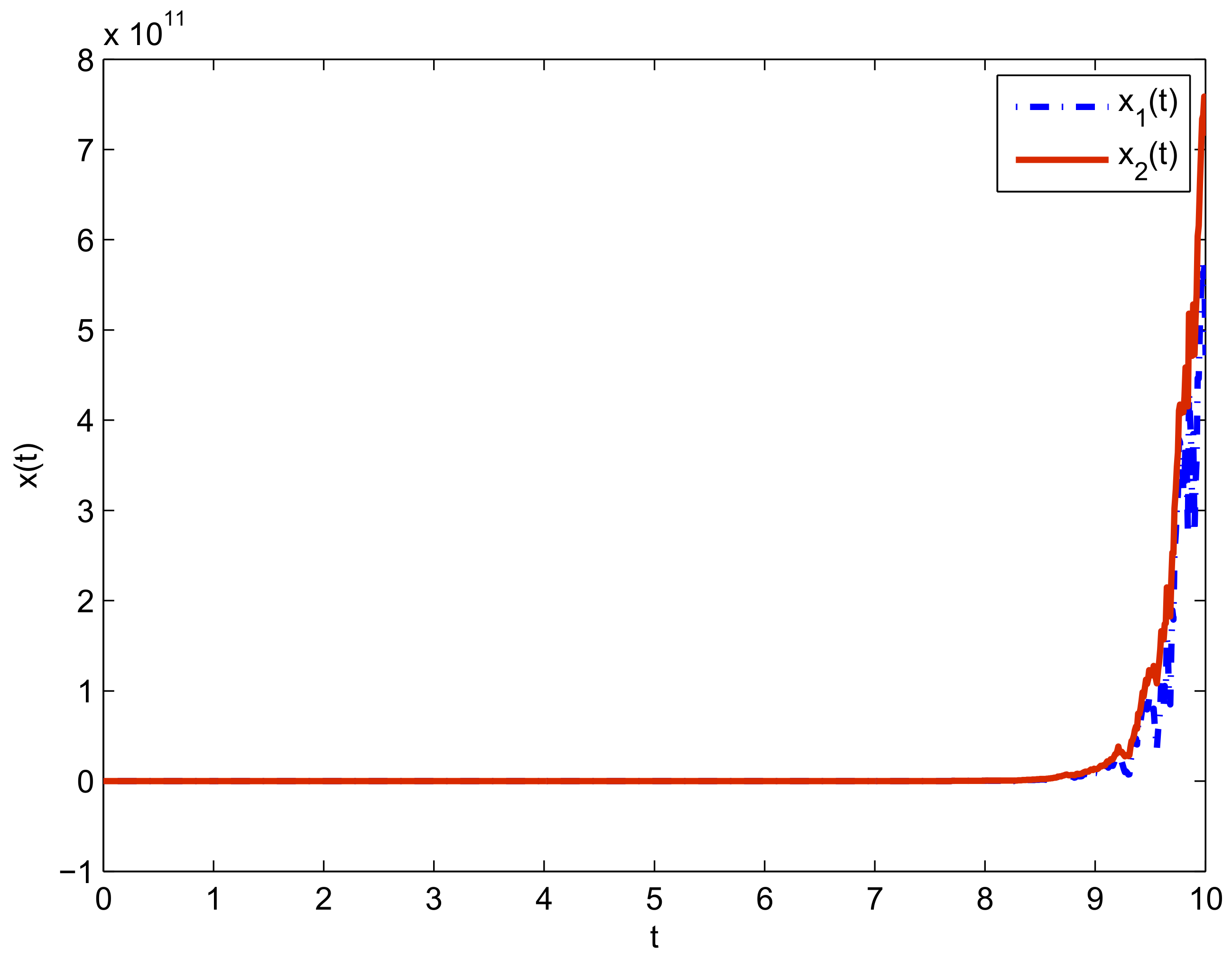
One can verify directly that the system (1) with the above matrices is not stable by Corollary 1. The system state trajectories are shown in Figure 2.

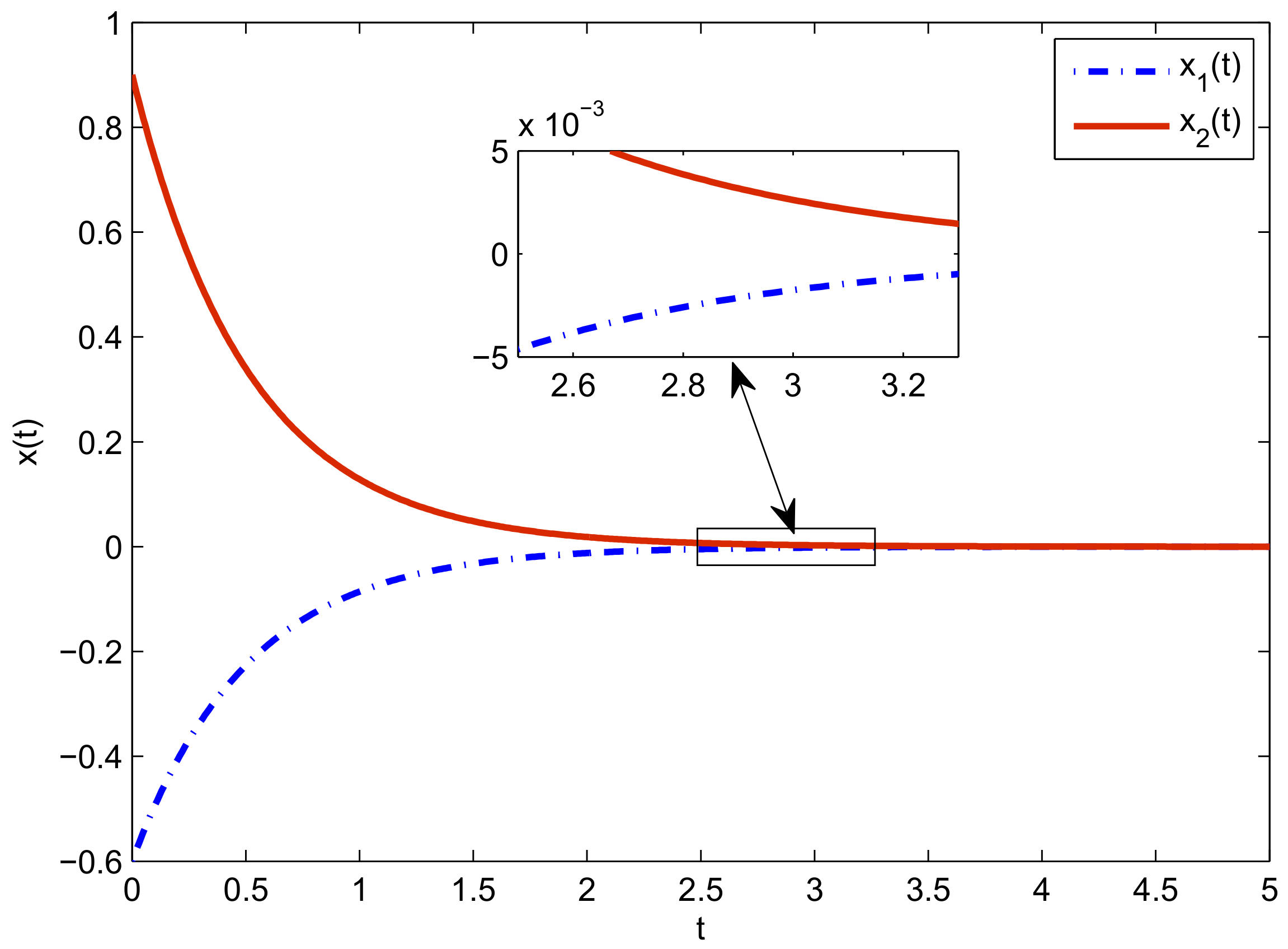
Using the common stabilization method, the system controllers are solved by Corollary 3:

$$\begin{array}{ccc}\hfill u_1\left(t\right)& =& K_{11}x\left(t\right)+K_{12}x(t-\nu \left(t\right)),\hfill \\ \hfill u_2\left(t\right)& =& K_{13}x\left(t\right)+K_{14}x(t-\nu \left(t\right)),\hfill \end{array}$$

where

$$K_{11}=\left[\begin{array}{cc}-4.7996& 5.8397\\ -0.5601& -4.8998\end{array}\right],K_{12}=\left[\begin{array}{cc}-1.0769& 3.2308\\ -0.5769& -2.769\end{array}\right],$$

$$K_{13}=\left[\begin{array}{cc}1.0000& -0.0833\\ -1.000& -0.6676\end{array}\right],K_{14}=\left[\begin{array}{cc}1.4167& 4.7500\\ -1.6667& -3.0000\end{array}\right].$$

The trajectories of the closed-loop system are shown in Figure 3. When $t\ge 2.8\left(s\right)$, $|x_i\left(t\right)|<5\times {10}^{-3}(i=1,2)$.

Remark 9.

Using the usual system stabilization method, only one pair of controllers $u_1\left(t\right)$ and $u_2\left(t\right)$ was designed, which can only play a calming role and can do nothing to adjust the dynamic performance.

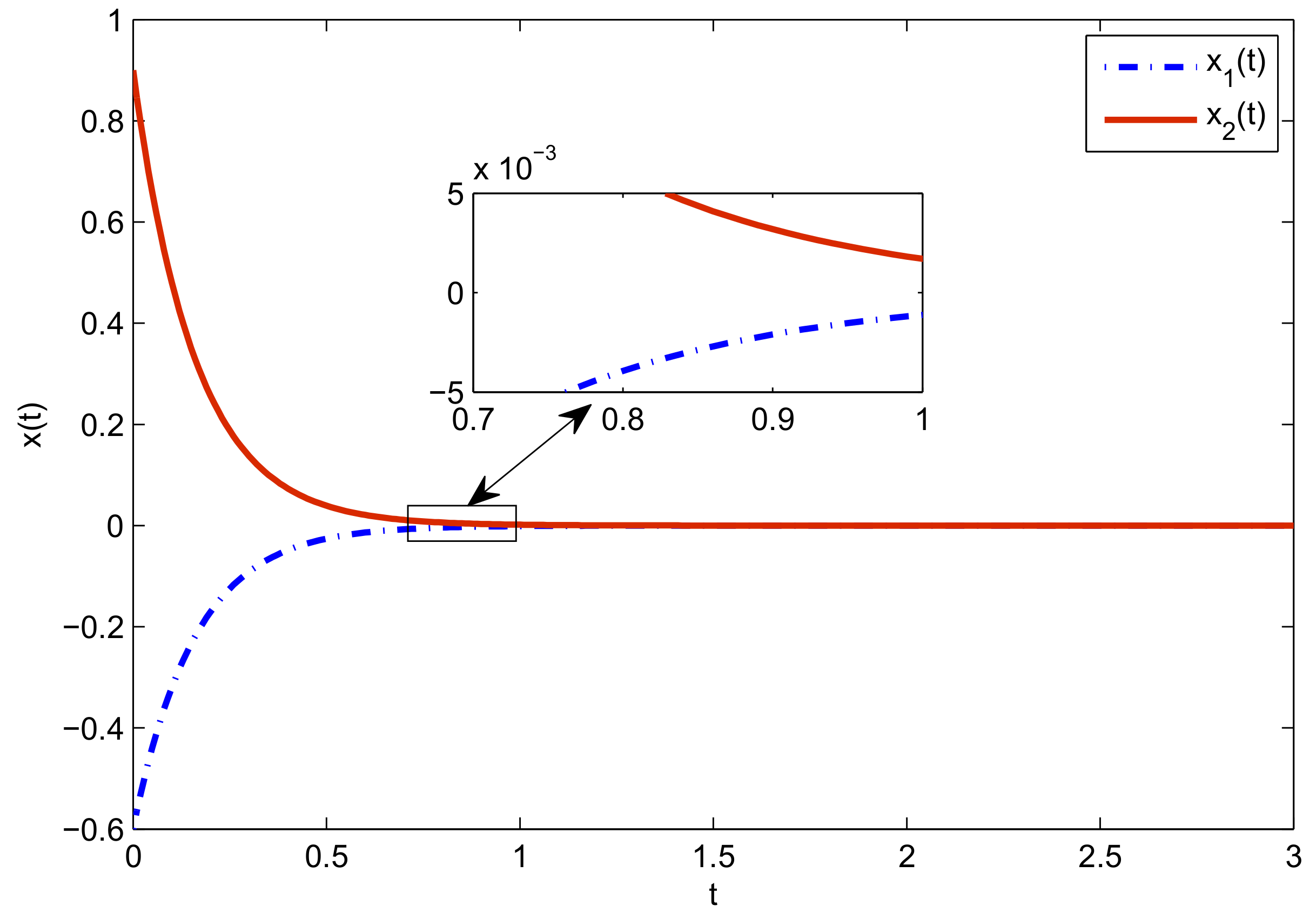
According to Theorem 3, we can control the convergence rate by setting different intervals. For example, let $(-b,-a)=(-6.5,-6)$ and $d=6$; the following controller can be obtained.

$$\begin{array}{ccc}\hfill u_3\left(t\right)& =& K_{21}x\left(t\right)+K_{22}x(t-\nu \left(t\right)),\hfill \\ \hfill u_4\left(t\right)& =& K_{23}x\left(t\right)+K_{24}x(t-\nu \left(t\right)),\hfill \end{array}$$

where

$$K_{21}=\left[\begin{array}{cc}-21.435& 19.1480\\ 4.4305& -13.217\end{array}\right],K_{22}=\left[\begin{array}{cc}-1.0769& 3.2308\\ -0.5769& -2.769\end{array}\right],$$

$$K_{23}=\left[\begin{array}{cc}1.0000& -0.0833\\ -1.000& -0.6676\end{array}\right],K_{24}=\left[\begin{array}{cc}1.4167& 4.7500\\ -1.6667& -3.0000\end{array}\right].$$

Under the controllers $u_3\left(t\right)$ and $u_4\left(t\right)$, the system state trajectories are shown in Figure 4. The eigenvalues of the closed-loop system are −6.2819 and −6.2728. Accordingly, the convergence speed of the system is significantly faster than that under the controllers $u_1\left(t\right)$ and $u_2\left(t\right)$. When $t>0.85\left(s\right)$, $|x_i\left(t\right)|<5\times {10}^{-3}(i=1,2)$.

What is more, the convergence rate can be slowed down though setting the parameter interval $(-1,-0.5)$. By Theorem 3, the controllers are obtained.

$$\begin{array}{ccc}\hfill u_5\left(t\right)& =& K_{31}x\left(t\right)+K_{32}x(t-\nu \left(t\right)),\hfill \\ \hfill u_6\left(t\right)& =& K_{33}x\left(t\right)+K_{34}x(t-\nu \left(t\right)),\hfill \end{array}$$

where

$$K_{31}=\left[\begin{array}{cc}-0.2811& 2.2249\\ -1.9157& -2.6406\end{array}\right],K_{32}=\left[\begin{array}{cc}-1.0769& 3.2308\\ -0.5769& -2.769\end{array}\right],$$

$$K_{33}=\left[\begin{array}{cc}1.0000& -0.0833\\ -1.000& -0.6676\end{array}\right],K_{34}=\left[\begin{array}{cc}1.4167& 4.7500\\ -1.6667& -3.0000\end{array}\right].$$

The eigenvalues of the closed-loop system are −0.7731 and −0.7732. Under the controllers $u_5\left(t\right)$ and $u_6\left(t\right)$, the system state trajectories are shown in Figure 5. As $t>7\left(s\right)$, $|x_i\left(t\right)|<5\times {10}^{-3}(i=1,2)$.

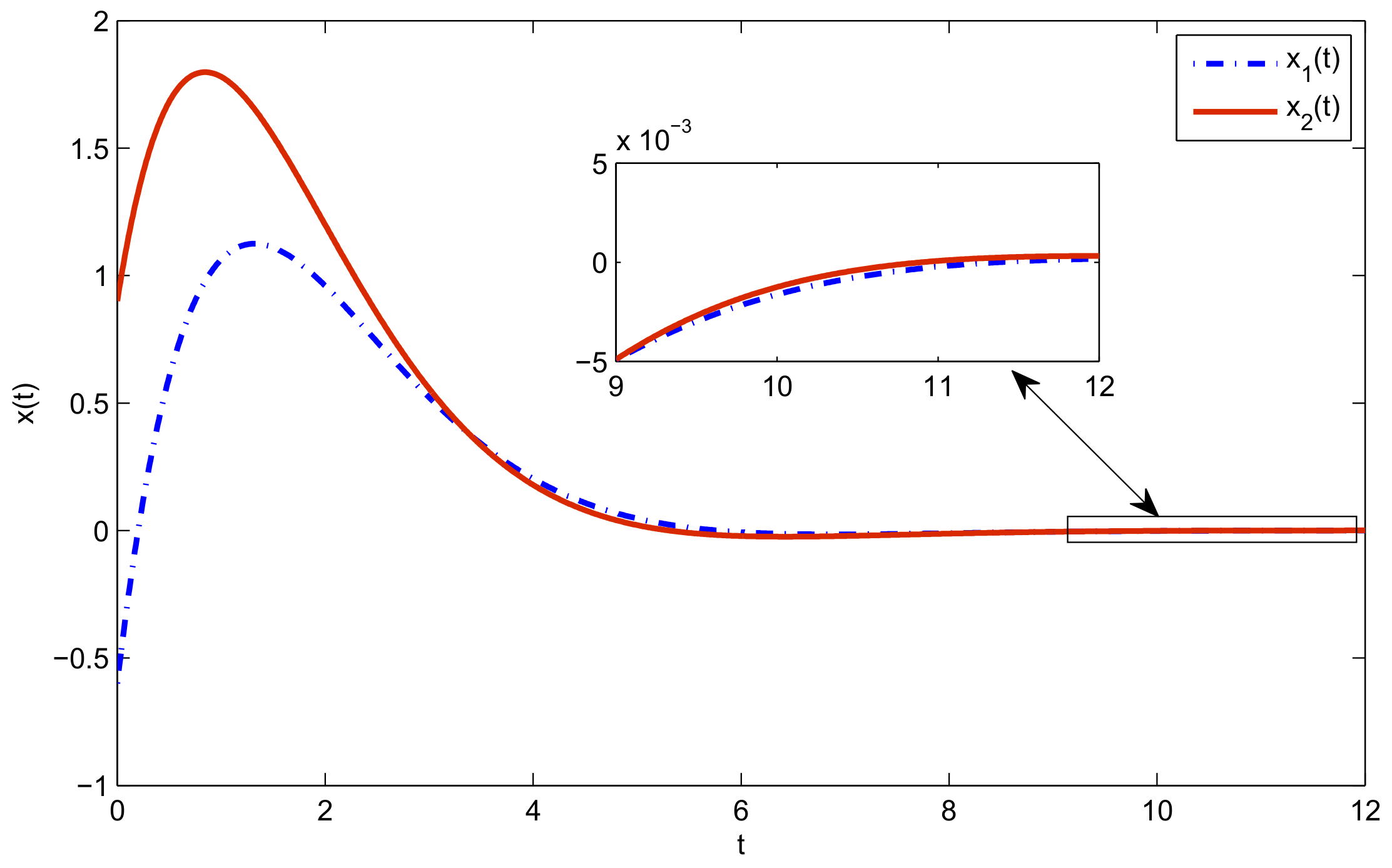
The method in this paper can not only accurately regulate the convergence speeds, but also other control dynamic properties. For simplicity, we only adjusted the damping performance of the system on the interval $(-1,-0.5)$.

According to Remark 4, $c=0.5625$ and $d=1.7250$ when the convergence interval is $(-1,-0.5)$. According to Algorithm 1, we obtain the following controllers.

$$\begin{array}{ccc}\hfill u_7\left(t\right)& =& K_{41}x\left(t\right)+K_{42}x(t-\nu \left(t\right)),\hfill \\ \hfill u_8\left(t\right)& =& K_{43}x\left(t\right)+K_{44}x(t-\nu \left(t\right)),\hfill \end{array}$$

where

$$K_{41}=\left[\begin{array}{cc}-0.9314& 3.3076\\ -4.0787& -0.9104\end{array}\right],K_{42}=\left[\begin{array}{cc}-1.0769& 3.2308\\ -0.5769& -2.7692\end{array}\right],$$

$$K_{43}=\left[\begin{array}{cc}1.0000& -0.0833\\ -1.000& -0.6676\end{array}\right],K_{44}=\left[\begin{array}{cc}1.4167& 4.7500\\ -1.6667& -3.0000\end{array}\right].$$

They ensure that the eigenvalues are at the minimum edge of the region. This group of controllers transforms the original over-damped system into an under-damped system, which is shown in Figure 6. The eigenvalues of the closed-loop system are $-0.7734+0.5625i$ and $-0.7734-0.5625i$.

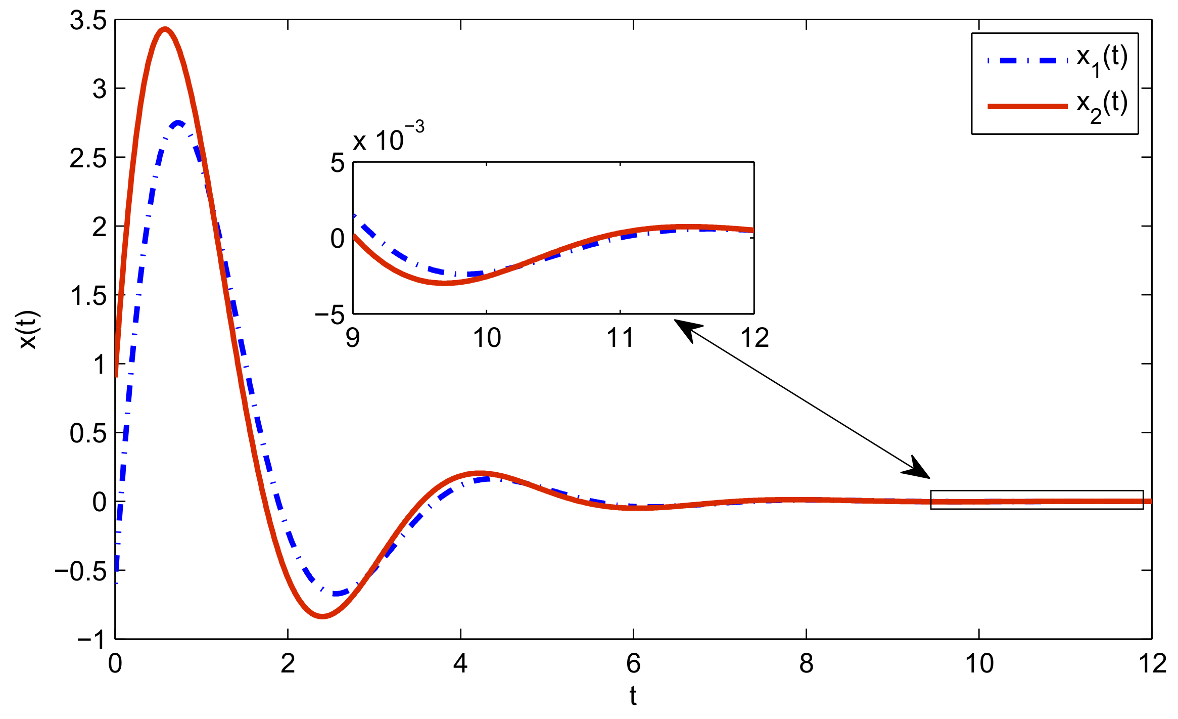
Certainly, the eigenvalues could be adjusted to the maximum edge of the region. By Algorithm 1, the controllers are obtained as below.

$$\begin{array}{ccc}\hfill u_9\left(t\right)& =& K_{51}x\left(t\right)+K_{52}x(t-\nu \left(t\right)),\hfill \\ \hfill u_{10}\left(t\right)& =& K_{53}x\left(t\right)+K_{54}x(t-\nu \left(t\right)),\hfill \end{array}$$

where

$$K_{51}=\left[\begin{array}{cc}-2.2728& 5.5432\\ -8.5499& 2.6665\end{array}\right],K_{52}=\left[\begin{array}{cc}-1.0769& 3.2308\\ -0.5769& -2.7692\end{array}\right],$$

$$K_{53}=\left[\begin{array}{cc}1.0000& -0.0833\\ -1.000& -0.6676\end{array}\right],K_{54}=\left[\begin{array}{cc}1.4167& 4.7500\\ -1.6667& -3.0000\end{array}\right].$$

The eigenvalues of the closed-loop system are $-0.7734+1.7250i$ and $-0.7734-1.7250i$. Under the controllers $u_9\left(t\right)$ and $u_{10}\left(t\right)$, the system state trajectories are shown in Figure 7.

Remark 10.

From Figure 4 to Figure 7, it can be seen that, with the adjustment of the closed-loop system eigenvalue, the dynamic performance of the system also changes accordingly. Therefore, it is very effective to control the performance of the system by adjusting the distributed eigenvalues.

Remark 11.

To highlight the waveform changes corresponding to the system state, the system eigenvalues are configured at the edges of two unconnected areas. In general, system eigenvalues are configured only within two unconnected areas.

7. Conclusions

In order to realize accurate control of the LSTDSs, this paper started by controlling the distribution area of the eigenvalues of the state matrix and reducing the influence of the time-delay terms and stochastic terms. Region stability was defined to describe the corresponding dynamic performance of the system. Region stability criteria and region stabilization conditions were given separately to judge the detailed stability characteristics and implement controller design. An algorithm was given to make up for the insufficiency of stabilization control. Finally, an instance was addressed to illustrate the accurate control of the new stabilization approach for the performance indicators of the LSTDSs.