Smooth Trajectory Planning at the Handling Limits for Oval Racing

Abstract

In motion planning for autonomous racing, the challenge arises in planning smooth trajectories close to the handling limits of the vehicle with a sufficient planning horizon. Graph-based trajectory planning methods can find the global discrete-optimal solution, but they suffer from the curse of dimensionality. Therefore, to achieve low computation times despite a long planning horizon, coarse discretization and simple edges that are efficient to generate must be used. However, the resulting rough trajectories cannot reach the handling limits of the vehicle and are also difficult to track by the controller, which can lead to unstable driving behavior. In this paper, we show that the initial edges connecting the vehicle’s estimated state with the actual graph are crucial for vehicle stability and race performance. We therefore propose a sampling-based approach that relies on jerk-optimal curves to generate these initial edges. The concept is introduced using a layer-based graph, but it can be applied to other graph structures as well. We describe the integration of the curves within the graph and the required adaptation to racing scenarios. Our approach enables stable driving at the handling limits and fully autonomous operation on the race track. While simulations show the comparison of our concept with an alternative approach based on uniform acceleration, we also present experimental results of a dynamic overtake with speeds up to 74 m/s on a full-size vehicle.

1. Introduction

Level 5 autonomous driving requires the safe handling of extreme situations in an unlimited operational design domain (ODD). One approach to address this and advance the state of the art is autonomous racing. Here, the autonomous driving software can be evaluated in a limited safe ODD in highly dynamic environments, and the findings can be generalized to road traffic scenarios [1]. While single-vehicle racing already poses a challenge due to the high speeds involved, autonomous multi-vehicle driving requires even more advanced planning concepts. The main challenges here are the high speeds and the dynamic environment. To handle these, motion planning must meet the following three requirements: First, trajectories close to the handling limits must be planned to fulfill time optimality, and it is necessary that these trajectories can be easily tracked by the controller. Second, a sufficiently long planning horizon is required to ensure recursive feasibility, i.e., that a feasible solution can be found in the next planning cycle. Third, low computation times are essential to allow fast reactions in the highly dynamic environment.

1.1. Related Work

In motion planning, a fundamental distinction is made between path and trajectory planning. While a path contains only spatial information such as the position and heading of the vehicle, a trajectory additionally takes into account temporal information such as time, velocity and acceleration. A further distinction is made between global, local and behavioral planning. We stick here to the definition in [2], which puts the terms in the context of racing. Global planning provides an optimal path or trajectory around the entire race track without considering opposing vehicles, where the optimization objective can be time [3,4] or geometric properties as curvature [5]. This optimal trajectory, also referred to as racing line, is usually determined offline and serves as the target for local planning. As an optional intermediate stage between global and local planning, there is behavioral planning, in which high-level maneuvers are planned that can reduce the search space of the local planning. Finally, the local planning itself takes into account the dynamic environment and plans collision-free trajectories with a limited planning horizon. [2]

There are several options to classify the local planning methods. We follow the categorization according to Paden et al. [6], which distinguishes between variational methods, incremental search techniques and graph search methods. In variational methods, as used in [7,8] for racing scenarios, a cost function is minimized by numerical optimization. It is advantageous that the state space is not discretized, but due to the non-convex structure of a local planning problem, the global optimal solution is not necessarily found. Therefore, these methods are often used for the re-optimization of already planned rough trajectories [9]. Incremental search techniques gradually build a progressively finer graph through sampling. These approaches are probabilistically complete, but computation time is in general not bounded. Most of these methods are based on rapidly-exploring random trees (RRT) [10], such as the RRT* [11] and RRT${}^{\mathrm{X}}$ [12]. For racing, an application is presented in [13]. Graph search methods are used to perform a search for the optimal solution within a graph, allowing them to find a global discrete-optimal solution also for non-convex problems. Often, these approaches are used only for path planning with a subsequent different velocity planning approach, since adding temporal dimensions to the graph can lead to the curse of dimensionality [14]. In order to achieve acceptable computation times despite the additional temporal dimensions, it is necessary to use a coarse discretization and a simplified edge structure. However, this is at the expense of the controller performance, as it has difficulty tracking such coarse trajectories. In addition to the classical graphs with a subsequent graph search, the sampling-based planning methods also belong to the category of graph search methods. For example, Werling et al. [15] generate jerk-optimal trajectories by sampling in the lateral and longitudinal direction. However, the resulting quartic or quintic polynomials used there allow only for simple maneuvers, which prevent complex movements with long planning horizons.

Stahl et al. [16] propose a graph-based local planning approach for racing scenarios. They discretize the race track by spatial nodes arranged in layers and connect them by edges generated out of cubic polynomials. However, since only the spatial domain is discretized, it is a path planning approach that requires subsequent velocity planning. While this path-velocity decomposition (PVD) is not critical for known static environments, it leads to conservative behavior in dynamic environments. Especially at high speeds, a large area of the race track would have to be blocked to avoid collisions. Planning based on a spatio-temporal graph, where the path and velocity profile are generated simultaneously, does not exhibit this conservative behavior.

McNaughton et al. [17] present an approach to extend a spatial graph with temporal dimensions for trajectory planning on highways. Instead of discretizing the temporal dimensions, they introduce intervals. Edges whose terminal states are in the same interval are reduced to a single edge, limiting the number of edges that need to be generated, countering the curse of dimensionality. The edges of the graph are generated online by sampling uniform accelerations on fixed paths, resulting in discontinuous acceleration profiles. As we will show, the coarse structure of the resulting trajectories has a disadvantageous effect on vehicle stability and race performance and thus requires adaptation to the racing scenario.

1.2. Contribution and Outline of the Paper

Graph-based trajectory planning approaches have the elementary advantage of being able to find the global discrete-optimal solution to non-convex problems. However, approaches that use PVD can lead to conservative behavior in dynamic environments, so extending a spatial graph by the temporal dimensions is desirable. In order to achieve both a sufficiently long planning horizon and a low computation time despite the added dimensions, a coarse graph discretization and simple constructed edges that can be generated efficiently must be chosen. For example, the approach in [17] to extend a spatial graph is based on fixed paths with uniform acceleration profiles within an edge. The simplicity of these edges allows for a long planning horizon, but it leads to coarse trajectories that cannot reach the handling limits of the vehicle and are difficult to track accurately by the controller, which can affect vehicle stability.

In this paper, we address this problem by treating the initial edges which connect the estimated state of the vehicle to the actual graph differently from the remaining edges within the graph. Since the initial edges correspond to the part of the planned trajectory that is actually traversed, they are decisive for the race performance and stability of the vehicle. The remaining edges are not affected and can have a simpler structure to obtain a long planning horizon and low computation times. We propose a sampling-based approach to generate the initial edges for racing scenarios, which are based analogously to [15] on the idea of jerk-optimal curves. We introduce our approach using the graph structure in [16], but it can also be applied to other graph structures by slight adjustment of the end conditions. The main contributions of this paper lie in the following aspects:

1.

The main idea is to treat the initial edges differently from the other edges in a spatio temporal graph. Our sampling-based approach for the generation of the initial edges uses jerk-optimal curves, whose smoothness reduces lateral acceleration deflections and thus increases vehicle stability, especially during braking maneuvers.

2.

We propose a concept for the selection of the end conditions of the jerk-optimal curves in order to adapt the initial edges to the racing scenario and thus get closer to the handling limits of the vehicle. We introduce the concept using the already proposed graph structure described in [16].

Our approach has been tested on a full-size race car within the software stack of the TUM Autonomous Motorsports team at the events of Indy Autonomous Challenge (IAC) and the Autonomous Challenge at CES (AC@CES), where both single- and two-vehicle races have been held. At the IAC on October 2021, high-speed laps were accomplished on the Indianapolis Motor Speedway (IMS) with an average speed of 60 m/s. In addition, an evasion maneuver with static obstacles was performed at a speed of 30 m/s. At the AC@CES in January 2022, overtaking maneuvers with speeds of up to 74 m/s were achieved on the Las Vegas Motor Speedway (LVMS), which is shown in Figure 1.

The remainder of this paper is structured as follows: In Section 2.1, the Frenét frame and the graph structure used here are introduced followed by the planning framework in which our concept is embedded in Section 2.2. The necessary identification of the start state from which the initial edge generation starts is described in Section 2.3. The detailed explanation of our proposed sampling-based approach for the generation of the initial edges is given in Section 2.4, and the results are shown in Section 3. While the architecture of the entire software stack used for the results is briefly described in Section 3.1, simulative and experimental results are shown in Section 3.2 and Section 3.3. Finally, the proposed approach is discussed in Section 4, and future work is addressed.

2. Material and Methods

2.1. Frenét Frame and Graph Structure

Our concept is introduced using the spatial graph structure proposed in [16] that covers the closed race track. However, it should be noted that our approach can be applied to other graph structures with minor modifications. The graph used here is generated along a reference line, which is defined as a sampled curve $[x_{\mathrm{r}}\left(s\right),y_{\mathrm{r}}\left(s\right),{\theta }_{\mathrm{r}}\left(s\right),{\kappa }_{\mathrm{r}}\left(s\right)]$ parameterized by arc length s. The position $r\left(s\right)=(x_{\mathrm{r}}\left(s\right),y_{\mathrm{r}}\left(s\right))$ of the reference line is given in Cartesian coordinates. ${\theta }_{\mathrm{r}}\left(s\right)$ is the angle for the corresponding arc length and ${\kappa }_{\mathrm{r}}\left(s\right)$ is the curvature. The spatial graph is defined in the Frenét coordinate system, which is given by the tangential and normal vector $t_{\mathrm{r}}$, $n_{\mathrm{r}}$ along the reference line. In this frame, each point $p(s,d)$ on the race track can uniquely be described by the longitudinal progress s along the reference line and the lateral distance d to it [18]:

$$p(s,d)=r\left(s\right)+d·n_{\mathrm{r}}\left(s\right)$$

(1)

The spatial nodes of the graph are generated perpendicular to the reference line with a fixed lateral distance at specific longitudinal progressions $s_m$, where m denotes the index of the discrete longitudinal coordinate (Figure 2a). We define a layer $L_m$ as the set of all spatial nodes with the same progress $s_m$. A spatial node $n_i$ is defined by the vector $[x_i,y_i,{\theta }_i]$ consisting of the individual position and heading, where i is the index of a spatial node in the layer. The heading ${\theta }_i$ is determined by linear interpolation between the heading of the according track boundary and the heading of a predefined racing line. In addition to the layers on the race track, layers can also be generated in the pitlane to allow operation in the pit. In case of a necessary entry or exit to or from the pitlane, it is possible to switch between the race track and pitlane layers.

In [16], the nodes of one layer are connected to those of the subsequent layer by spatial edges, creating a closed graph around the race track and enabling path planning. Trajectory planning requires an additional extension of the presented spatial graph by the temporal dimension. However, since our concept is independent of these two steps, we do not specify those further here.

The resulting spatio-temporal graph can be used directly for trajectory planning when the start state of the search matches a node of the graph. However, since in reality, the start state will not be exactly on a node, it must be connected to the spatio-temporal graph before the actual graph search. The initial edges $E_0$ connecting the start state to the graph in both spatial and temporal dimensions are exemplarily shown in Figure 2b. The layer chosen to generate the initial edges $E_0$ is referred to as the initial layer $L_{\mathrm{init}}$ and may change at each planning cycle. Each initial edge, or alternatively a subset of them, can then be expanded according to a subsequent graph search by generating the remaining edges $E_1$.

2.2. Local Planning Framework

Trajectory planning based on a spatio-temporal graph consists of the three steps shown in Figure 3. The first step is to identify the start state from which to start the actual planning process. This does not necessarily have to be the estimated state of the vehicle. Second, the start state must be connected to the used graph structure by creating initial edges $E_0$. Since the initial edges in general cover a longer time horizon than the calculation time of a whole planning cycle, the initial edges are the part of the trajectory that is actually traversed by the race car and thus are elementary for the vehicle stability and race performance. Once the start state is connected to the graph, the third step is to search the remaining graph for the optimal trajectory that satisfies the desired planning horizon. For this step, a suitable cost function and an efficient graph search algorithm are necessary.

In this paper, we address the start state identification (Section 2.3) and in particular the generation of the initial edges (Section 2.4) for racing scenarios. Our approach generates several initial edges that allow stable driving close to the handling limits. However, the initial edges cannot be used without the subsequent graph search, since they do not satisfy the required planning horizon needed for recursive feasibility [16]. Therefore, the approach proposed here requires a concept for a subsequent efficient graph search that finds the solution within the non-convex environment while guaranteeing the required planning horizon.

2.3. Start State Identification

The selection of the start state is crucial for the overall race performance. Since the planned trajectory serves as the reference for the tracking controller, the estimated state of the vehicle cannot be used directly as the start state. This would cause the reference trajectory to follow the actual vehicle state, which would not allow a control error to build up and thus provide no incentive for the controller to follow the trajectory. Instead, as shown in Figure 4, we project the estimated state onto the previously planned trajectory, allowing a control error to accumulate. However, since the vehicle moves during trajectory generation, using the projected state as the start state would result in jumping trajectories between consecutive planning cycles. To avoid this, similar to [19], a part of the previously planned trajectory is kept constant, and the start state is placed at the end of this constant part. We keep the part constant that corresponds to the expected computation time required for the planning cycle, which allows for a continuous transition between two successively planned trajectories.

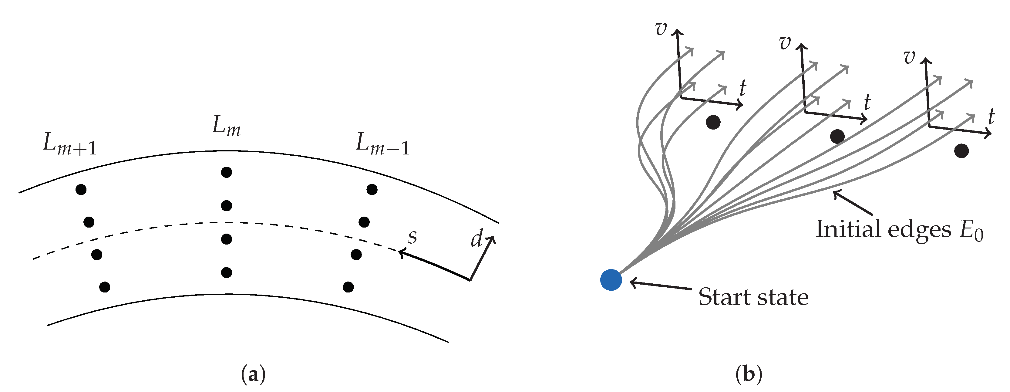
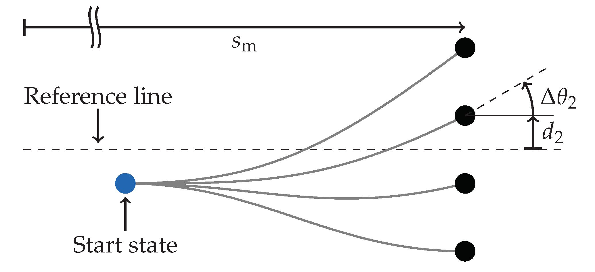
2.4. Initial Edge Generation

Our proposed concept for the generation of the initial edges is a sampling-based approach that connects the start state to the spatio-temporal graph. The generation is performed in the Frenét frame, so that at the beginning of a planning cycle, the Cartesian coordinates of the start state have to be transformed into the Frenét coordinates. Using this start state as initial conditions, we sample end conditions in the Frenét frame to produce a set of lateral and longitudinal jerk-optimal curves. We rely on jerk-optimal curves since jerky trajectories can excite neglected high-frequency dynamics in the tracking controller, resulting in a decrease in vehicle stability. The end conditions of the curves must be chosen to integrate the initial edges into the graph structure and achieve high performance for racing scenarios. After the generation, the lateral and longitudinal curves are transformed back into Cartesian coordinates to perform collision and feasibility checks.

2.4.1. Coordinate Transformation

A trajectory dependent on time t described in Cartesian coordinates consists of the position ($x\left(t\right),y\left(t\right)$), the heading $\theta \left(t\right)$, the curvature $\kappa \left(t\right)$, the velocity $v\left(t\right)$ and the acceleration $a\left(t\right)$. The needed transformation between Frenét coordinates and Cartesian coordinates $[s,\dot{s},\ddot{s},d,\dot{d},\ddot{d}]\left(t\right)\to [x,y,\theta ,\kappa ,v,a]\left(t\right)$ is derived in [15] and can be stated in closed form. By inverting these equations, the back transformation $[x,y,\theta ,\kappa ,v,a]\left(t\right)\to [s,\dot{s},\ddot{s},d,\dot{d},\ddot{d}]\left(t\right)$ can also be obtained in closed form with the exception of s. However, the longitudinal position s can be determined by using a projection method as in [20]. Inaccuracies resulting from the coordinate transformation can be neglected here due to the low curvatures of the considered oval race tracks.

2.4.2. Jerk-Optimal Movement

We generate the lateral curves $d\left(t\right)$ and the longitudinal curves $s\left(t\right)$ each based on a jerk-optimal movement. This reduces abrupt acceleration changes, which has a beneficial effect on the system stability. Ref. [21] shows that the curve $c\left(t\right)$, which minimizes the cost functional

$$J\left(c\left(t\right)\right)=\frac{1}{2}{\int }_{t_0}^{t_{\mathrm{e}}}{\stackrel{⃛}{c}}^2\left(t\right)\mathrm{d}t$$

(2)

and satisfies the initial condition $[c\left(t_0\right),\dot{c}\left(t_0\right),\ddot{c}\left(t_0\right)]$ at the start time $t_0$ and the fixed end condition $[c\left(t_{\mathrm{e}}\right),\dot{c}\left(t_{\mathrm{e}}\right),\ddot{c}\left(t_{\mathrm{e}}\right)]$ at the end time $t_{\mathrm{e}}$, is a quintic polynomial:

$$c\left(t\right)=p_5{t}^5+p_4{t}^4+p_3{t}^3+p_2{t}^2+p_{1}t+p_0$$

(3)

The parameters $p_0$ to $p_5$ can be efficiently computed as shown in [22], which makes the operation on the vehicle possible. It should be noted that although jerk-optimal initial edges are generated, the selection of the optimal sequence of edges in the subsequent graph search can be performed with a different cost function adapted to the racing scenario.

2.4.3. Integration into Graph Structure

Since the generated polynomials have to be embedded as initial edges in the graph structure, a simple equidistant sampling of the end conditions is not possible. Instead, the end conditions must be sampled so that the edges end up in the initial layer $L_{\mathrm{init}}$ with the appropriate individual position $(x_i,y_i)$ and heading ${\theta }_i$ of each spatial node $n_i$. The initial layer $L_{\mathrm{init}}$ is selected as the first layer that exceeds a speed-dependent minimum distance in the direction of travel. These distance values increase with rising speed in order to avoid high curvature values and the associated unfeasible lateral accelerations. They are determined empirically and stored in a lookup table.

Figure 5 shows schematically the needed spatial end conditions of the initial edges. The spatial nodes in the initial layer are arranged perpendicular to the reference line and therefore have the same longitudinal position $s_{\mathrm{m}}$. Hence, the end position of the longitudinal curve has to be chosen accordingly without sampling. To ensure that the edges terminate in the nodes, the lateral end position must be sampled according to the lateral position of each spatial node $d_i$, where i is again the index of a spatial node $n_i$ in the initial layer $L_{\mathrm{init}}$.

Analogous to the lateral position, $\Delta {\theta }_i={\theta }_i-{\theta }_{\mathrm{r}}\left(s_{\mathrm{m}}\right)$ refers to the heading of the i-th spatial node relative to the reference line. In addition to the position, this individual heading of a spatial node at the end of an edge must also be guaranteed. This is completed by correctly specifying the end conditions of the velocity $\dot{d}\left(t_{\mathrm{e}}\right)$ and $\dot{s}\left(t_{\mathrm{e}}\right)$. Instead of specifying the lateral and longitudinal velocities directly, we sample the global velocity to cover the entire possible velocity range. Finer sampling is applied in the high velocity range due to the lower engine power at high speeds. For this, we divide the entire velocity range into two intervals with a different number of equidistant distributed velocity samples: $[v_1,\dots ,v_N,\dots ,v_{N+M}]$. N denotes the number of samples in the low speed range and M the number in the high range. To assure the individual heading of a node, each velocity sample $v_j$ is then transformed into the corresponding lateral and the longitudinal velocity ${\dot{d}}_{ij}$, ${\dot{s}}_{ij}$, where j indicates the corresponding velocity sample index. According to the transformation from Cartesian to Frenét coordinates in [15], the lateral and longitudinal velocities are obtained by:

$$\begin{array}{cc}\hfill {\dot{s}}_{ij}& =v_j\frac{cos\Delta {\theta }_i}{1-{\kappa }_{\mathrm{r}}\left(s_{\mathrm{m}}\right)d_i}\hfill \end{array}$$

(4)

$$\begin{array}{cc}\hfill {\dot{d}}_{ij}& ={\dot{s}}_{ij}\left[-{\kappa }_{\mathrm{r}}\left(s_{\mathrm{m}}\right)d_i\right]tan\Delta {\theta }_i\hfill \end{array}$$

(5)

With that, the end conditions on the position and velocity are specified, and the end conditions on time $t_{\mathrm{e}}$ and acceleration $\ddot{s}\left(t_{\mathrm{e}}\right)$, $\ddot{d}\left(t_{\mathrm{e}}\right)$ remain.

2.4.4. Performance Improvement for Racing-Scenarios

In sampling-based methods for traffic scenarios, the lateral and longitudinal accelerations at the end time $t_{\mathrm{e}}$ are often set to 0 m/s² for comfort reasons. In the context of a racing scenario, however, this is undesirable. For example, in an acceleration maneuver, the initial edges would have to adapt at an early stage to fulfill the end conditions, resulting in a loss of race performance. Simple equidistant sampling of the end acceleration and the end time is also not possible due to the curse of dimensionality and the accompanying computing time. Instead, reducing the number of samples without sacrificing race performance is desired.

We tackle this problem by determining one suitable pair of end acceleration $a_{ij}$ and end time $t_{\mathrm{e},ij}$ for each spatial node $n_i$ combined with a velocity sample $v_j$. This avoids additional sampling of the acceleration dimension besides the spatial node and the end velocity. The determined acceleration in Cartesian coordinates $a_{ij}$ is then transformed into the corresponding curvilinear accelerations ${\ddot{s}}_{ij}$ and ${\ddot{d}}_{ij}$ serving as end conditions of the lateral and longitudinal movement. Rearranging the transformation equations from [15], yields to the following required expressions:

$$\begin{array}{cc}\hfill {\ddot{s}}_{ij}& =\frac{1}{1-{\kappa }_{\mathrm{r}}\left(s_l\right)d_i}\left[a_{ij}cos\Delta {\theta }_i-{\dot{d}}_{ij}\left({\kappa }_i{v}_j-{\kappa }_{\mathrm{r}}\left(s_{\mathrm{m}}\right){\dot{s}}_{ij}\right)+\left({\kappa }_{\mathrm{r}}^{\prime }\left(s_{\mathrm{m}}\right)d_i{\dot{s}}_{ij}^2+{\kappa }_{\mathrm{r}}\left(s_{\mathrm{m}}\right){\dot{d}}_{ij}{\dot{s}}_{ij}\right)\right]\hfill \end{array}$$

(6)

$$\begin{array}{cc}\hfill {\ddot{d}}_{ij}& =\frac{{\ddot{s}}_{ij}}{{\dot{s}}_{ij}}{\dot{d}}_{ij}-{\dot{s}}_{ij}^2\left[tan\Delta {\theta }_i\left({\kappa }_{\mathrm{r}}^{\prime }\left(s_{\mathrm{m}}\right)d_i+{\kappa }_{\mathrm{r}}\left(s_{\mathrm{m}}\right)\frac{{\dot{d}}_{ij}}{{\dot{s}}_{ij}}\right)-\frac{1-{\kappa }_{\mathrm{r}}\left(s_{\mathrm{m}}\right)d_i}{{cos}^2\Delta {\theta }_i}\left({\kappa }_i\frac{1-{\kappa }_{\mathrm{r}}\left(s_{\mathrm{m}}\right)d_i}{cos\Delta {\theta }_i}-{\kappa }_{\mathrm{r}}\left(s_{\mathrm{m}}\right)\right)\right]\hfill \end{array}$$

(7)

These equations show that not only the curvature of the reference line ${\kappa }_{\mathrm{r}}\left(s_{\mathrm{m}}\right)$ but also its derivative ${\kappa }_{\mathrm{r}}^{\prime }\left(s_{\mathrm{m}}\right)$ with respect to the arc length s must be known. In addition, a curvature ${\kappa }_i$ at the end of an edge must be specified, which we choose as the curvature of the reference line on the initial layer $L_{\mathrm{init}}$.

Determining the end acceleration $a_{ij}$ and the associated end time $t_{\mathrm{e},ij}$ for each pair of spatial node $n_i$ and velocity sample $v_j$ is now the critical part for the race performance. Our approach to this is based on the consideration that in most racing scenarios, the optimal behavior is to accelerate or decelerate as much as possible. Therefore, we generate the initial edges as close as possible to a uniform accelerating edge by choosing the uniform acceleration and the corresponding end time as end conditions. Unlike fixed spatial edges with uniform acceleration profiles, this approach retains the advantage of the jerk-optimality, which reduces the load on the tracking controller.

The uniform acceleration required traversing a path of length $\Delta s_{ij}$ from a starting velocity $v_0$ to the desired velocity sample $v_j$ within the time $T_{ij}=t_{\mathrm{e},ij}-t_0$ can be derived from the uniform acceleration equations. Accordingly, the end acceleration and end time is determined by:

$$\begin{array}{cc}\hfill a_{ij}& =\frac{v_j-v_0}{T_{ij}}\hfill \end{array}$$

(8)

$$\begin{array}{cc}\hfill T_{ij}& =\frac{2\Delta s_{ij}}{v_j+v_0}\hfill \end{array}$$

(9)

For the evaluation of Equation (9), the length $\Delta s_{ij}$ of an edge is needed. However, the actual distance cannot be determined, as prior to the generation of an edge, its length is not known. We therefore perform an additional step to approximate the length $\Delta s_{ij}$ before generating the edges. Since the paths of edges ending in the same spatial node are of similar length, only one length per node $n_i$ is determined and employed for all end velocities $v_j$. For this, a single edge is generated for each spatial node $n_i$, and its length is used as an approximation of $\Delta s_{ij}$. These edges are only used to approximate the path lengths and are therefore discarded after generation. We choose the end conditions of these temporary edges such that they end with the pose of the corresponding spatial node $n_i$ and with the maximum velocity $v_{N+M}$. Furthermore, the end acceleration is set to zero, and the end time is calculated according to Equation (9) with the Euclidean distance between the start position and the considered spatial node as the length. The exact selection of these values is not crucial, since we are only interested in the length.

The described selection of end accelerations $a_{ij}$ and end times $t_{\mathrm{e},ij}$ results in initial edges that resemble uniformly accelerated motion but adhere to the initial conditions while preserving jerk-optimality. The velocity profiles of these initial edges are shown in Figure 6 for exemplary sampled end velocities $v_j$. It can be seen that the velocity profiles of edges with similar start and end accelerations are closer to the uniform acceleration. However, the more the start acceleration deviates from the end acceleration, the more curved the velocity profile becomes in order to comply with all boundary conditions.

A reduction in computation time for the proposed sampling-based approach can be achieved by precalculating the transformation of all sampling points. Since the spatial nodes $n_i$ of the graph and the velocity samples $v_j$ can be calculated offline, the end conditions for position and velocity in Frenét coordinates can also be precalculated and stored for online use. In contrast, the end acceleration $a_{ij}$ and end time $T_{ij}$ from Equations (8) and (9) cannot be precomputed due to the need for the start velocity, which is not known offline. Hence, the end acceleration and end time including the approximation of $\Delta s_{ij}$ are determined online. Since the calculation of (6) and (7) requires more complex calculations, these are precalculated offline for sampled Cartesian accelerations. As these sampled values do not match the $a_{ij}$ calculated online from (8), we use the end conditions calculated from the sample closest to $a_{ij}$.

2.4.5. Stopping to Standstill

One challenge with the proposed approach is stopping at arbitrary positions, which is necessary for fully autonomous operation on the race track. Since the initial edges $E_0$ always end in spatial nodes $n_i$ within the layers, it is only possible to specify a velocity of zero at these spatial nodes. Due to the need to stop at any position in case of a pit stop or a blocked track, an additional node is generated online with zero velocity and placed in each planning cycle depending on the current scenario. When the vehicle is requested to the pitlane, this stop node is placed in the pit, and if static objects block the road, it is placed in front of these objects.

When a stop is requested and the distance to the stop node falls below a certain threshold, the local planner solely plans to this node using the initial edges without a subsequent graph search. However, the initial edge generation has a short planning horizon, which means that no feasible edges to the stop node can be generated at high speeds. While this problem does not occur during a pit stop due to the low speeds, in the case of a blocked road, it is countered by the farsighted graph search, which guides the initial edges by slowing down early. In case of a stop on the race track due to the race rules, however, there is no concrete stop position. Instead, the target speed is set to 0 m/s, slowing down the vehicle based on the cost function, and the stop vertex is placed at the end of the previously planned trajectory in each cycle until a solution to standstill is found.

If the distance between the start state and end node is too small while braking to a fixed position, our approach leads to unfeasibly high accelerations. We avoid this behavior by preventing a new planning below a distance threshold of 5 m. Instead, we repeatedly send the last planned trajectory to the tracking controller until the vehicle comes to a stop at the desired position.

3. Results

In this section, we show in simulative (Section 3.2) and experimental results (Section 3.3) how our sampling-based approach for the generation of the initial edges affects vehicle stability and race performance. All results were obtained using the software stack described in Section 3.1. The spatial graph was parameterized with a longitudinal layer distance of 75 m and a lateral node resolution of 1.4 m. For our sampling-based approach, 50 velocity samples and 50 offline calculated acceleration values were used. The minimum planning horizon was set to 5 s. Our planning approach is implemented in Python 3.8 with single C-functions. The scenarios were conducted on the LVMS, a 2480 m oval race track with a curved mainstretch, a straight backstretch and four turns.

3.1. Autonomous Driving Software Architecture

As described in Section 2.2, a graph search must follow the initial edge generation to meet the needed planning horizon. For all results, an approach analogous to the concept in [17] is used for the graph search. We rely on this, since it is a well-known concept for highway scenarios, which is close to the racing scenario. This concept is based on the efficient generation of edges with uniform acceleration profiles sampled along the fixed spatial paths computed offline. The cost function used in our graph search is composed of four weighted terms. The first two terms penalize the spatial and speed deviation from a predefined global racing line in order to follow the racing line during solo driving. If a speed limit defined by the race rules exists, this is used instead of the racing line speed target. For multi-vehicle driving, the third term punishes edges that lie within an ellipse-shaped area surrounding the predicted opponents. Last, the peak curvature is weighted, favoring low-curvature overtaking maneuvers. A detailed description of the search algorithm and the used cost function can be found in [23].

The local planning concept consisting of the proposed sampling-based initial edge generation and the above graph search is integrated within the overall software stack of the TUM Autonomous Motorsports team. It is a sequential architecture consisting of a localization, perception, tracking, prediction, local planning and control module. We address only the local planning interfaces here and refer to [24] for more details.

Based on the estimated state provided by the localization module and the prediction of the detected dynamic obstacles by the prediction module, the local planning module generates a collision-free and feasible trajectory and forwards it to the tracking controller. The planning of the trajectory also requires information about the race track map, a reference line and the desired racing line, which are computed in advance by the global planning module proposed in [4] and the mapping module. Finally, there is the control module, which is based on a Tube-MPC and is described in [25]. It re-optimizes the planned trajectory and determines the throttle, steering and braking commands to realize the behavior specified in the target trajectory.

3.2. Simulation Results

In this section, we compare our sampling-based approach for the generation of the initial edges $E_0$ with the uniform acceleration approach in [17], which we already use for the edges $E_1$ within the graph search. Thus, in the comparison approach, the same concept based on fixed spatial edges with sampled uniform acceleration profiles is used for both the edges within the graph search and the initial edge generation. We choose to compare with [17], since the direct comparison shows the changes that result from a different treatment of the initial edges compared to a simpler initial edge generation. In contrast to the uniform acceleration approach, the proposed sampling-based approach achieves jerk-optimal transitions that take the initial conditions into account. Another advantage of our approach is the individual paths for each initial edge. Unlike in [17], where different acceleration profiles are based on the same underlying path, in our approach, each path is unique, since the spatial and temporal information are generated simultaneously by combining the lateral and longitudinal movement. This adjusts the path to match the temporal information, resulting in lower lateral accelerations.

We compare the proposed sampling-based approach with the uniform acceleration approach in three different scenarios related to race performance and vehicle stability. For the uniform acceleration approach, 50 equidistant distributed acceleration values were applied for each spatial edge generated. All scenarios were simulated on an 8-core AMD Ryzen 7 Pro 4750U laptop with 1.7 GHz and 32 GB RAM.

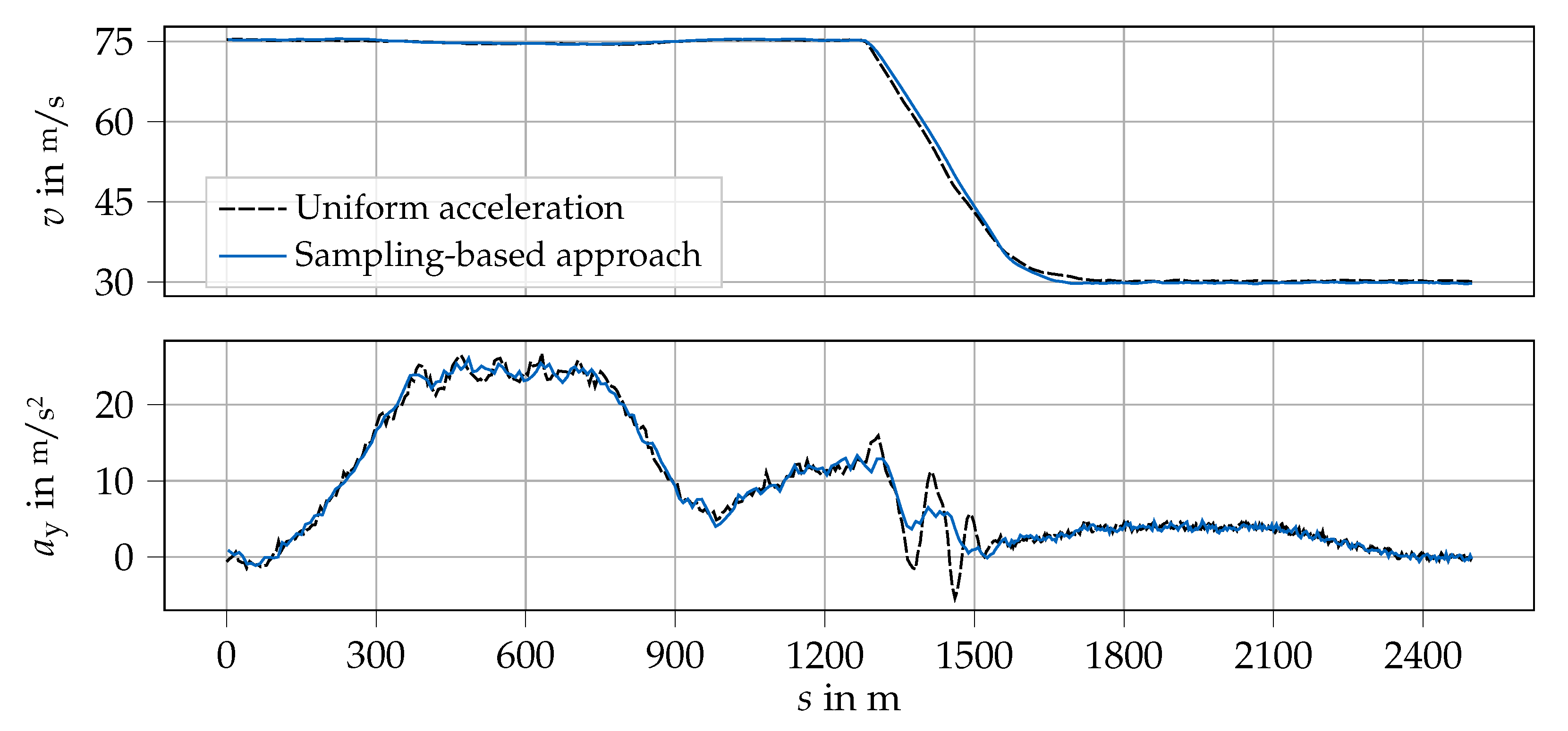
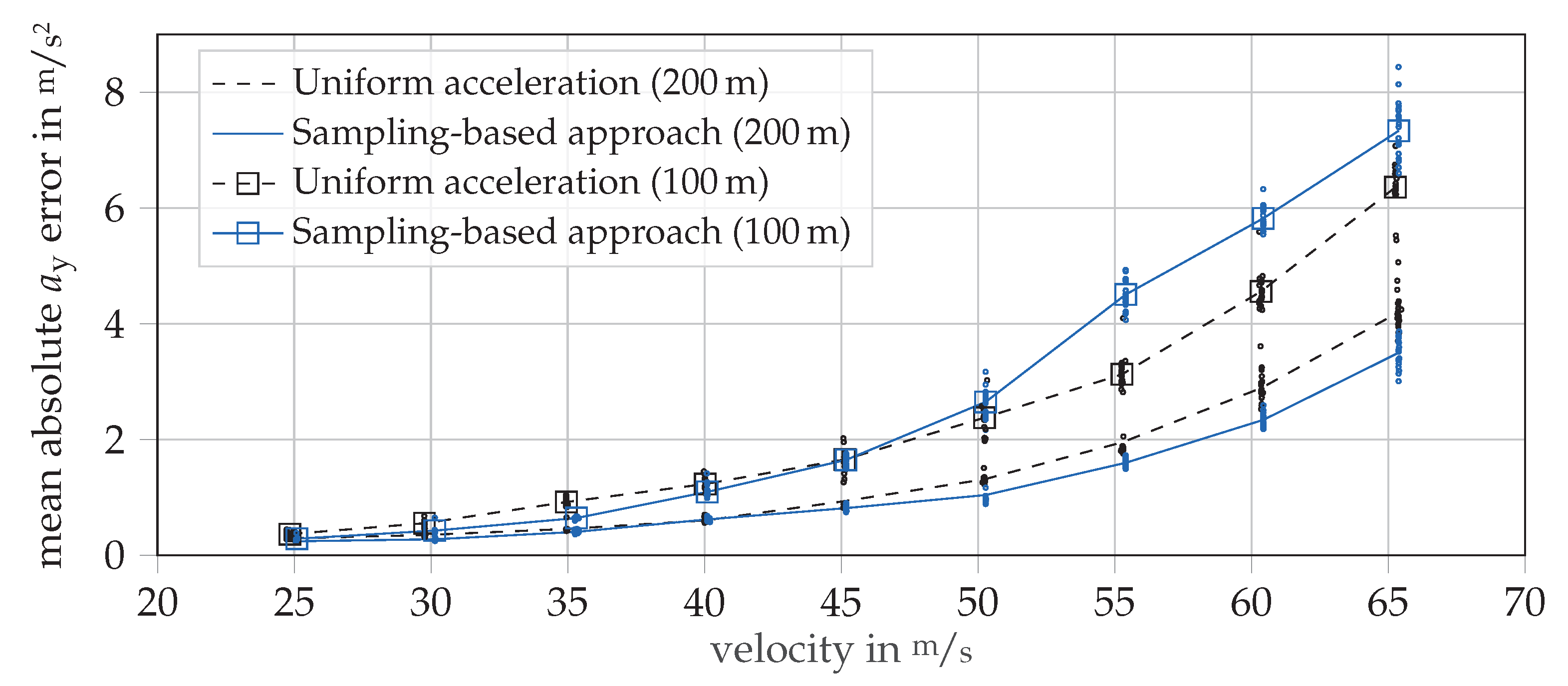
3.2.1. Single-Vehicle Driving

First, we consider single-vehicle driving on the racing line with no speed restrictions, which allows for the fastest possible lap. Starting with a standing start followed by twenty flying laps, the resulting lap times are shown in

Table 1. Lap time comparison for single-vehicle driving on the LVMS.

	Standing Start Lap	Flying Lap (Mean/Variance)
Uniform acceleration	47.814 s	30.431 s/0.001 s2
Sampling-based approach	51.854 s	30.001 s/0.004 s2

. The corresponding velocity v and lateral acceleration $a_{\mathrm{y}}$ profiles are shown in Figure 7 for the standing start lap and the first flying lap (beginning at 2480 m). It can be seen that the starting behavior of our sampling-based approach is not as performant as the uniform acceleration approach, resulting in a higher lap time. This is because high acceleration profiles can be generated in the uniform acceleration approach from the beginning, regardless of the start acceleration of 0 m/s². The sampling-based approach, on the other hand, produces a transition from zero acceleration to higher accelerations. However, since only flying starts are decisive in the competition formats of IAC and AC@CES, this disadvantage at standing starts was not pursued further.

In the case of flying laps, the sampling-based approach results in higher speeds, especially in the turns, and thus lower lap times. Higher speeds in the curves can be achieved due to the previously described simultaneous generation of spatial and temporal information and the accompanying lower lateral accelerations. Furthermore, the lateral acceleration profile shows that the use of the sampling-based approach also leads to a steadier behavior of the vehicle in the curves. Particularly at the exit of the fourth curve (2200 m and 4600 m), the uniform acceleration shows strong deflections, which even lead to a lateral acceleration contrary to the direction of the curve. Since the uniform acceleration approach leads to higher lateral accelerations, no sufficiently curved edge can be found in the corresponding planning cycles that does not exceed the friction limits, leaving only barely curved edges.

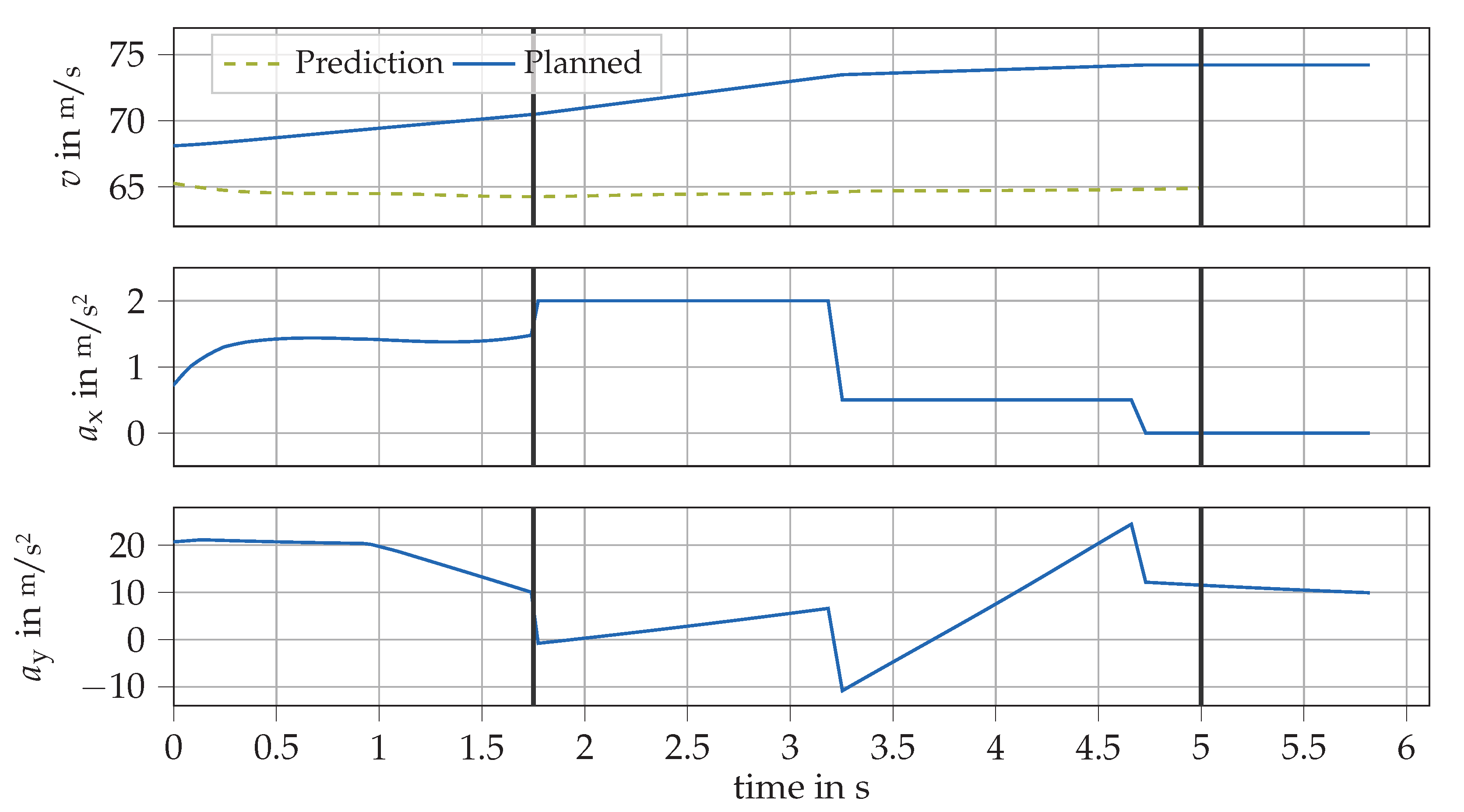
3.2.2. Braking Maneuver

Braking to standstill or decelerating to a lower speed is essential for race track operation. For example, after a fast lap, it is necessary to slow down to a lower speed in order to drive safely into the pitlane. For an exemplary braking maneuver from 75 m/s to a target speed of 30 m/s, the resulting velocity v and lateral acceleration $a_{\mathrm{y}}$ profiles are shown in Figure 8. Although the velocity profile during deceleration looks similar for both approaches, significant oscillations can be observed in the lateral acceleration profile of the uniform acceleration approach. These lateral deflections become larger as the start and target speed difference increases, which can ultimately lead to unstable vehicle behavior.

If the same maneuver is performed without a subsequent tracking controller, but with an exactly assumed tracking, these lateral oscillations do not occur to the same extent. The oscillations are therefore not planned by the uniform acceleration approach, but result from the interference of the planned trajectories and the Tube-MPC, which has difficulty tracking the rough trajectories despite re-optimization. The sampling-based approach, on the other hand, creates smoother trajectories that are easier to track by the controller, resulting in a more stable driving behavior.

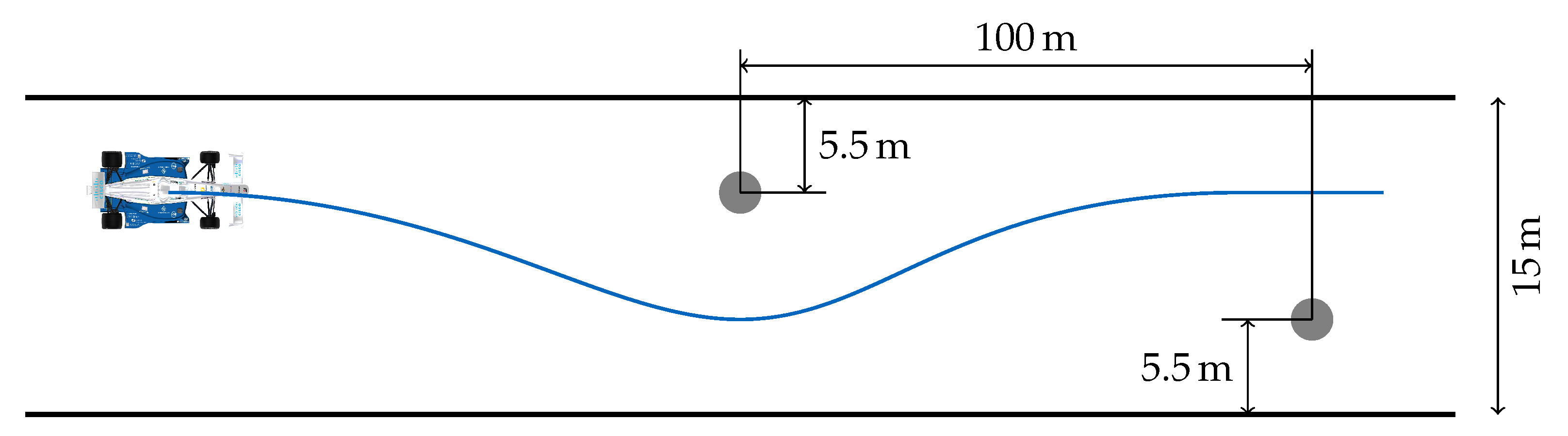
3.2.3. Object Evasion

Static obstacles on the race track require a quick reaction and safe evasion. The behavior during such a maneuver is examined here using the scenario from Figure 9 with two static objects arranged on opposite sides. Since the difficulty of object evasion increases with rising ego velocity, the described scenario is run with velocities in steps of five in the interval from 25 m/s to 65 m/s in each case twenty times. Furthermore, the detection range has a decisive influence on the difficulty, so we compare the behavior at a low range of 100 m and a higher range of 200 m. It should be noted that a global racing line within the inner half of the track (upper half in Figure 9) is used, forcing an outward and inward movement.

All tested evasive maneuvers were successful, i.e., collision-free. In addition to this success rate, the average absolute control error between the re-optimized target by the Tube-MPC and the actual lateral acceleration $a_{\mathrm{y}}$ is crucial, as this is an indication of vehicle stability (Figure 10). It is noticeable that for higher target speeds, the actual vehicle speed is slightly higher than targeted. This is not due to the planned trajectories but to the Tube-MPC, which tends to drive faster than planned at high speeds. Furthermore, it can be seen that with a detection range of 200 m, the sampling-based approach leads to lower control errors than the uniform acceleration approach at the same range. This is particularly noticeable at high speeds. With a detection range of 100 m, however, another effect can be observed. While at lower speeds, the sampling-based approach leads again to lower errors than the uniform acceleration approach, this changes above a speed of 45 m/s. This is due to the lower computation time of the uniform acceleration approach and the associated ability to react faster to environmental changes. Higher computation times and thus less remaining distance to react lead to higher lateral accelerations and larger control errors. However, the results shown here cannot be generalized to every evasion maneuver. Due to the fixed layers in the spatial graph, the planning behavior depends on the position of the obstacles relative to the layers, so the overall behavior may differ.

3.3. Experimental Results

The proposed approach was evaluated in single- and two-vehicle scenarios on a full-scale autonomous race car at IAC and AC@CES. For all events, the Dallara AV-21 race car (Figure 1) was used, which is based on a modified version of the Indy Lights chassis. It includes an 8-core Intel Xeon E-2278GE CPU with 64 GB RAM, with the local planning module running on one core. The planner achieves an average computation time of 95 ms for a whole planning cycle using the discretization described at the beginning of Section 3. Since the highest speeds were achieved during the final of the AC@CES on the LVMS, we present only these results.

The final of the AC@CES was an overtaking competition in which two vehicles alternate overtaking maneuvers at increasing speeds. The vehicle to be overtaken must drive as the defender on the inside of the race track and maintain a certain speed. The overtaking vehicle must follow the defender with a longitudinal distance of more than 30 m and overtake the defender after entering the passing zone. Due to the distance to be maintained before the actual overtaking process, the detection range does not have a major impact on the local planner, in contrast to the results from Section 3.2.3.

The actual velocity v and lateral acceleration $a_{\mathrm{y}}$ profiles of the last two overtaking maneuvers of the TUM Autonomous Motorsports team are shown in Figure 11. In addition, the target speed, which is used in the cost function, and the period in which passing is allowed are indicated. Braking despite increased target speeds ($s \approx 700 \mathrm{m}$ and $s \approx 6100 \mathrm{m}$) results from the passing restriction. In this case, the target speed is invalidated and the distance to the opposing vehicle is maintained instead. If passing is allowed, the respective overtaking maneuver is initiated and the target speed is targeted accordingly. The deviation between actual and target speed after the acceleration process does not result from the planned trajectory but from the control error within the Tube-MPC. Figure 11 shows that the entire competition consists of acceleration, deceleration and overtaking maneuvers at high speeds. By using the proposed sampling-based approach for the generation of the initial edges, the advantageous behavior shown in Section 3.2 can be achieved in the individual maneuvers with respect to vehicle stability and race performance.

The planned motion of the time step marked in Figure 11 with an ego speed of up to 74 m/s is shown in Figure 12. The defender is predicted with a constant speed of about 65 m/s on the inside of the race track. The sampling-based approach connects the start state to the chosen initial layer with an horizon of 1.7 s, while the minimum planning horizon of 5 s is achieved by the subsequent graph search. The resulting trajectory performs an overtaking maneuver due to the cost function, which penalizes edges close to the dynamic obstacle. With the graph search based on uniform accelerations, the rough course of the trajectory is noticeable for times from 1.7 s. In contrast, at the beginning of the trajectory, i.e., at the initial edge, a smooth transition of the longitudinal acceleration $a_{\mathrm{x}}$ curve can be recognized. A video of the final overtaking maneuver and other scenarios from the IAC and AC@CES can be found in [26].

Figure 12. Predicted opponent velocity and planned ego motion for the time step marked in Figure 11. The end of the initial edge and the minimum planning horizon of 5 s are indicated by black vertical lines.

Figure 12. Predicted opponent velocity and planned ego motion for the time step marked in Figure 11. The end of the initial edge and the minimum planning horizon of 5 s are indicated by black vertical lines.

4. Discussion and Conclusions

This paper addresses the challenges of online graph-based trajectory generation for racing scenarios. The proposed sampling-based approach for the generation of the initial edges connecting the vehicle’s estimated state with the actual graph enables smoothly planned trajectories and thus stable driving at high speeds close to the handling limits of the vehicle. The approach is independent of the used graph structure and the subsequent graph search. Thus, the remaining edges within the graph search can be roughly discretized and have a simplified structure, so that, in addition to stability and race performance, the requirements on the planning horizon and the computation time can be met. In addition, our approach allows for holistic operation on the race track through the ability to stop at arbitrary positions such as the pit. Experiments on a full-scale vehicle show that our approach can avoid static objects as well as overtake dynamic objects at speeds up to 74 m/s. Simulative results show that lower lap times on flying starts and lower lateral acceleration oscillations during braking maneuvers can be achieved, resulting in an increased vehicle stability. With a detection range of 200 m, our sampling-based approach also results in smaller control errors and thus more stable evasion maneuvers. However, if only a smaller detection range of 100 m is available, the higher computing time of the sampling-based approach impacts more strongly, which in turn leads to larger control errors at high-speed evasion maneuvers. A reduction of the computation time can be achieved by a heuristic that samples only a reduced number of end velocities without sacrificing race performance. For instance, the actually realizable accelerations can be utilized to select only a subset of all end velocities. A lower computation time would also allow online generation of the spatial part of the graph. That would make the sampling-approach independent of fixed layers and thus the planned trajectories independent of the current position.

References

1. Jiang, A. Research on the Development of Autonomous Race Cars And Impact on Self-driving Cars. J. Phys. Conf. Ser. 2021, 1824, 012009. [Google Scholar] [CrossRef]
2. Betz, J.; Zheng, H.; Liniger, A.; Rosolia, U.; Karle, P.; Behl, M.; Krovi, V.; Mangharam, R. Autonomous Vehicles on the Edge: A Survey on Autonomous Vehicle Racing. IEEE Open J. Intell. Transp. Syst. 2022, 3, 458–488. [Google Scholar] [CrossRef]
3. Herrmann, T.; Christ, F.; Betz, J.; Lienkamp, M. Energy Management Strategy for an Autonomous Electric Racecar using Optimal Control. In Proceedings of the 2019 IEEE Intelligent Transportation Systems Conference (ITSC), Auckland, New Zealand, 27–30 October 2019; pp. 720–725. [Google Scholar] [CrossRef]
4. Christ, F.; Wischnewski, A.; Heilmeier, A.; Lohmann, B. Time-optimal trajectory planning for a race car considering variable tyre-road friction coefficients. Veh. Syst. Dyn. 2021, 59, 588–612. [Google Scholar] [CrossRef]
5. Heilmeier, A.; Wischnewski, A.; Hermansdorfer, L.; Betz, J.; Lienkamp, M.; Lohmann, B. Minimum curvature trajectory planning and control for an autonomous race car. Veh. Syst. Dyn. 2020, 58, 1497–1527. [Google Scholar] [CrossRef]
6. Paden, B.; Čáp, M.; Yong, S.Z.; Yershov, D.; Frazzoli, E. A Survey of Motion Planning and Control Techniques for Self-Driving Urban Vehicles. IEEE Trans. Intell. Veh. 2016, 1, 33–55. [Google Scholar] [CrossRef] [Green Version]
7. Subosits, J.K.; Gerdes, J.C. From the Racetrack to the Road: Real-Time Trajectory Replanning for Autonomous Driving. IEEE Trans. Intell. Veh. 2019, 4, 309–320. [Google Scholar] [CrossRef]
8. Liniger, A.; Domahidi, A.; Morari, M. Optimization-based autonomous racing of 1:43 scale RC cars. Optim. Control Appl. Methods 2015, 36, 628–647. [Google Scholar] [CrossRef] [Green Version]
9. Dolgov, D.; Thrun, S.; Montemerlo, M.; Diebel, J. Path Planning for Autonomous Vehicles in Unknown Semi-structured Environments. Int. J. Robot. Res. 2010, 29, 485–501. [Google Scholar] [CrossRef]
10. LaValle, S.M. Rapidly-Exploring Random Trees: A New Tool for Path Planning; Technical Report 98-11; Iowa State University, Department of Computer Science: Ames, IA, USA, 1998. [Google Scholar]
11. Karaman, S.; Frazzoli, E. Optimal Kinodynamic Motion Planning using Incremental Sampling-based Methods. In Proceedings of the 49th IEEE Conference on Decision and Control (CDC), Atlanta, GA, USA, 15–17 December 2010; pp. 7681–7687. [Google Scholar] [CrossRef]
12. Otte, M.; Frazzoli, E. RRTX: Real-Time Motion Planning/Replanning for Environments with Unpredictable Obstacles. In Algorithmic Foundations of Robotics XI; Akin, H.L., Amato, N.M., Isler, V., van der Stappen, A.F., Eds.; Springer International Publishing: Cham, Switzerland, 2015; Volume 107, pp. 461–478. [Google Scholar] [CrossRef]
13. Jeon, J.h.; Cowlagi, R.V.; Peters, S.C.; Karaman, S.; Frazzoli, E.; Tsiotras, P.; Iagnemma, K. Optimal Motion Planning with the Half-Car Dynamical Model for Autonomous High-Speed Driving. In Proceedings of the 2013 American Control Conference, Washington, DC, USA, 17–19 June 2013; IEEE: Piscataway, NJ, USA, 2013; pp. 188–193. [Google Scholar] [CrossRef]
14. Kant, K.; Zucker, S.W. Toward Efficient Trajectory Planning: The Path-Velocity Decomposition. Int. J. Robot. Res. 1986, 5, 72–89. [Google Scholar] [CrossRef]
15. Werling, M.; Ziegler, J.; Kammel, S.; Thrun, S. Optimal Trajectory Generation for Dynamic Street Scenarios in a Frenét Frame. In Proceedings of the 2010 IEEE International Conference on Robotics and Automation, Anchorage, AK, USA, 3–7 May 2010; pp. 987–993. [Google Scholar] [CrossRef]
16. Stahl, T.; Wischnewski, A.; Betz, J.; Lienkamp, M. Multilayer Graph-Based Trajectory Planning for Race Vehicles in Dynamic Scenarios. In Proceedings of the 2019 IEEE Intelligent Transportation Systems Conference (ITSC), Auckland, New Zealand, 27–30 October 2019; pp. 3149–3154. [Google Scholar] [CrossRef]
17. McNaughton, M.; Urmson, C.; Dolan, J.M.; Lee, J.W. Motion Planning for Autonomous Driving with a Conformal Spatiotemporal Lattice. In Proceedings of the 2011 IEEE International Conference on Robotics and Automation, Shanghai, China, 9–13 May 2011; pp. 4889–4895. [Google Scholar] [CrossRef]
18. Carmo, M.P.d. Differential Geometry of Curves and Surfaces, 2nd ed.; Dover Publications Inc.: Mineola, NY, USA, 2016. [Google Scholar]
19. Ziegler, J.; Bender, P.; Dang, T.; Stiller, C. Trajectory Planning for Bertha—A Local, Continuous Method. In Proceedings of the 2014 IEEE Intelligent Vehicles Symposium Proceedings, Dearborn, MI, USA, 8–11 June 2014; pp. 450–457. [Google Scholar] [CrossRef]
20. Werling, M.; Groll, L. Low-level controllers realizing high-level decisions in an autonomous vehicle. In Proceedings of the 2008 IEEE Intelligent Vehicles Symposium, Eindhoven, The Netherlands, 4–6 June 2008; IEEE: Piscataway, NJ, USA, 2008; pp. 1113–1118. [Google Scholar] [CrossRef]
21. Takahashi, A.; Hongo, T.; Ninomiya, Y.; Sugimoto, G. Local Path Planning And Motion Control For Agv In Positioning. In Proceedings of the IEEE/RSJ International Workshop on Intelligent Robots and Systems’, (IROS ’89) ’The Autonomous Mobile Robots and Its Applications, Tsukuba, Japan, 4–6 September 1989; pp. 392–397. [Google Scholar] [CrossRef]
22. Werling, M.; Kammel, S.; Ziegler, J.; Gröll, L. Optimal trajectories for time-critical street scenarios using discretized terminal manifolds. Int. J. Robot. Res. 2012, 31, 346–359. [Google Scholar] [CrossRef]
23. Rowold, M.; Ögretmen, L.; Kerbl, T.; Lohmann, B. Efficient Spatio-Temporal Graph-Search for Local Trajectory Planning on Oval Race Tracks. Actuators 2022. accepted. [Google Scholar]
24. Betz, J.; Betz, T.; Fent, F.; Geisslinger, M.; Heilmeier, A.; Hermansdorfer, L.; Herrmann, T.; Huch, S.; Karle, P.; Lienkamp, M.; et al. TUM Autonomous Motorsport: An Autonomous Racing Software for the Indy Autonomous Challenge. arXiv 2022, arXiv:2205.15979. [Google Scholar] [CrossRef]
25. Wischnewski, A.; Herrmann, T.; Werner, F.; Lohmann, B. A Tube-MPC Approach to Autonomous Multi-Vehicle Racing on High-Speed Ovals. IEEE Trans. Intell. Veh. 2022. [Google Scholar] [CrossRef]
26. Chair of Automatic Control TUM. Smooth Trajectory Planning at the Handling Limits for Oval Racing. Available online: https://www.youtube.com/watch?v=H4tl_ggR1cc (accessed on 2 November 2022).
Figure 1. The Dallara AV-21 race cars of the TUM Autonomous Motorsports and TII EuroRacing team during the AC@CES on the LVMS.
Actuators 11 00318 g001
Figure 2. Used graph structure and initial edges. (a) Spatial nodes (black dots) of the graph are placed on layers perpendicular to the reference line (dashed line). (b) Initial edges E 0 connecting the start state to the initial layer L init in both the spatial and temporal dimensions.
Actuators 11 00318 g002
Figure 3. Framework of the proposed approach for the generation of the initial edges.
Actuators 11 00318 g003
Figure 4. The start state of the trajectory generation is determined by projecting the estimated state onto the previously planned trajectory and keeping constant the part corresponding to the average planning calculation time.
Actuators 11 00318 g004
Figure 5. Example initial edges (gray lines) connecting the start state (blue dot) with the initial layer and fulfilling the individual end pose of each spatial node (black dots). Coordinates are shown exemplarily for the second node.
Actuators 11 00318 g005
Figure 6. Comparison of velocity profiles generated by our sampling-based approach and uniform acceleration. Exemplarily, several end velocities from 0 to 80 m/s are sampled with a start velocity of 50 m/s and a start acceleration of 10 m/s.
Actuators 11 00318 g006
Figure 7. Comparison of our sampling-based approach and the uniform acceleration approach for a standing start and a flying lap on the LVMS.
Actuators 11 00318 g007
Figure 8. Sampling-based approach and uniform acceleration approach comparison for a braking maneuver from 75 m/s to 30 m/s on the mainstretch of the LVMS.
Actuators 11 00318 g008
Figure 9. Evasion scenario with two obstacles (gray) on the backstretch of the LVMS (not to scale).
Actuators 11 00318 g009
Figure 10. Mean absolute lateral acceleration control error per run (dots) using the sampling-based approach and the uniform acceleration approach with different ideally assumed detection ranges for the evasion maneuver shown in Figure 9. The lines represent the average values of the means.
Actuators 11 00318 g010
Figure 11. Last two overtaking maneuvers during the final of AC@CES on the LVMS. The permitted passing period is marked in red. The black vertical line indicates the time step shown in Figure 12.
Actuators 11 00318 g011