Article

Efficient Spatiotemporal Graph Search for Local Trajectory Planning on Oval Race Tracks

1
Automatic Control, Department of Mechanical Engineering, TUM School of Engineering and Design, Technical Universtiy of Munich, 85748 Garching, Germany
2
Institute of Automotive Technology, Department of Mechanical Engineering, TUM School of Engineering and Design, Technical Universtiy of Munich, 85748 Garching, Germany
*
Author to whom correspondence should be addressed.
Actuators 2022, 11(11), 319; https://doi.org/10.3390/act11110319
Submission received: 26 September 2022 / Revised: 26 October 2022 / Accepted: 28 October 2022 / Published: 3 November 2022
(This article belongs to the Special Issue Intelligent Control and Robotic System in Path Planning)

Abstract

:
Autonomous racing has increasingly become a research subject as it provides insights into dynamic, high-speed situations. One crucial aspect of handling these situations, especially in the presence of dynamic obstacles, is the generation of a collision-free trajectory that represents a safe behavior and is also competitive in the case of racing. We propose a local planning approach that generates such trajectories for a racing car on an oval race track by searching a spatiotemporal graph. A considerable challenge of search-based methods in a spatiotemporal domain is the curse of dimensionality. Therefore, we propose how a previously presented graph structure that is based on intervals instead of discrete values can be searched more efficiently without losing optimality by using a uniform-cost search strategy. We extend the search method to make it anytime-capable so that it can provide a suboptimal trajectory even if the search has to be terminated early. The graph-based planning approach allows us to apply a flexible cost function so that our approach can operate fully autonomously on an oval race track, including the pit lane. We present a cost function for oval racing and explain how the terms contribute to the desired behaviors. This is supported by results with a full-scale prototype.

1. Introduction

During the last decade, autonomous racing has drawn attention from different research groups. The motivation behind this is to learn from difficult dynamic situations at high velocities and transfer the knowledge to traffic scenarios, increasing future autonomous vehicles’ safety. Following the DARPA challenges [1,2], many planning and control approaches for racing have focused on the fastest lap for a single vehicle on a closed race track. Their capabilities, approaching the performance of human race drivers, have been demonstrated on full-scale prototypes, e.g., in [3,4] within the autonomous racing series Roborace [5]. While this application already poses challenges due to the high velocities and driving at the handling limits, even more difficult scenarios arise when multiple vehicles race simultaneously. The vehicles should react safely to one another and at the same time maintain a short lap time. Therefore, a local planning approach must generate a trajectory representing an appropriate behavior, which is often a compromise between conflicting objectives. The local environment must be considered, which includes the race track, track bounds, friction limits, and the likely motion of other vehicles. Combined with the high velocities in racing, these aspects present the following challenges that we will address in this paper:
(1)
The race track offers many maneuver variants to be considered, since the presence of other vehicles constitutes a nonconvex problem. A sufficiently long planning horizon is required and a short computation time is desired, which further complicates the search for the optimal solution.
(2)
One must ensure that the planning problem remains solvable in the next planning step. In the field of model predictive control (MPC) this is known as recursive feasibility. An illustrative example in the context of racing is a braking point before a sharp turn that, if not correctly determined, could lead to a planning problem with no feasible safe solution due to excessive speed at the turn entry.
(3)
The used cost function should result in safe but competitive behaviors in all scenarios.
(4)
Newly detected obstacles or falsely predicted vehicles require fast reactions. Therefore, the computation time for generating a trajectory in the new environment should be as short as possible.

1.1. Related Work

Most planning approaches that competed in the DARPA Grand Challenge (2005) [1] separate the trajectory generation into a path planning step and a subsequent velocity planning step to complete the trajectory. While a path only contains spatial information, meaning a sequence of poses, a trajectory also contains information about time and velocity at the corresponding poses, which is called spatiotemporal. The path-velocity decomposition (PVD) [6] is sufficient for environments with only static obstacles, but too conservative for dynamic obstacles. Traffic rules and simultaneous driving of the competitors prompted the teams of the DARPA Urban Challenge (2007) [2] to introduce new approaches for behavior and trajectory planning that consider the spatiotemporal aspect in the presence of dynamic obstacles. In the following years, various planning approaches have been proposed. Paden et al. [7] provided a comprehensive survey on the methods used, which they categorized into variational, graph search, and incremental methods. In the following, we present some approaches and use cases based on methods from the three categories relevant to our problem. They are generally designed for road traffic scenarios but solve a similar problem in environments with multiple static and dynamic obstacles and can be applied for an operation on a race track.
Variational methods formulate an optimal control problem (OCP) that is solved numerically using direct or indirect methods. Obstacles can enter the problem directly as constraints as in [8] or indirectly as in [9], such that a collision would result in high costs. In the context of racing, variational methods are often used to compute the racing line, i.e., the trajectory for a minimum lap time on a closed race track. While Veneri et al. [10] and Lovato et al. [11] used a point mass model constrained to a precalculated gg-envelope, Casanova [12] and Christ et al. [13] solved the minimum lap time OCP with detailed vehicle models. However, the racing line optimization does not consider obstacles and is therefore unsuitable for our use case with static and dynamic obstacles. Other approaches, as in [14,15], apply an online replanning scheme if the vehicle has to deviate from the offline generated racing line, e.g., to avoid an obstacle. The planning horizon is limited to a small section of the race track so that short computation times can be achieved. In general, variational methods are fast, especially when convex programming is applied, as was demonstrated in [16]. However, the planning problem in environments with obstacles is generally nonconvex, so numerical-optimization-based methods usually only find a local optimal solution depending on the initialization [14,17]. An illustrative example of nonconvexity in the racing context is an overtaking scenario with collision-free solutions on the left and the right side of another vehicle [18,19]. Including the temporal dimension or more vehicles adds a combinatorial aspect as many maneuver variants are possible [20]. Each maneuver can be a local optimal solution in a spatiotemporal state space. If sufficient computation resources are available, multiple OCPs can be solved in parallel as in the stitching method presented in [21] or for each homotopy class as in [22].
Graph search methods discretize the spatial or spatiotemporal state space and can find a global discrete-optimal solution to the nonconvex planning problem. For racing, Stahl et al. [23] created a spatial state lattice by placing nodes on layers distributed along the track and oriented perpendicular to a reference line. Each node corresponded to a pose of the vehicle. Edges associated with costs connected the nodes to complete the spatial graph and represent available paths. A search over multiple layers yielded the path with a planning horizon of at least 200 m , long enough to ensure recursive feasibility. A velocity planner based on a forward–backward solver [4] completed the final trajectory. Static obstacles could be considered by blocking edges and dynamic obstacles by selecting a so-called action template and using a PVD. Other graph search methods search in the spatiotemporal space and can therefore account for dynamic obstacles directly. The approach in [24] sampled time, velocity, and lateral displacement from a reference line and generated jerk-minimal trajectories to reach the discrete states. A recent approach in [25] extended the approach for the racing scenario and used a constant time horizon. However, Stahl et al. [23] argued that a one-step sampling approach could not plan complex maneuvers at high velocities, such as initiating an overtaking maneuver just before a sharp turn, because the shortsighted solution might not be recursively feasible. spatiotemporal approaches that can plan multiple steps ahead build a graph with usually two additional dimensions compared to the graph in [23]. Besides the pose, Ziegler and Stiller [26] discretized time and velocity to create a spatiotemporal state lattice and use quintic polynomials with the appropriate boundary conditions to generate jerk-minimal edges. Instead of discretizing time and velocity, McNaughton et al. [27] assigned time and velocity intervals to the spatial nodes to create spatiotemporal nodes. Sampling acceleration profiles along spatial edges during an exhaustive search yielded spatiotemporal edges whose end velocities and times could be assigned to the intervals. In addition to the interval-based graph structure, Morsali et al. [28] performed an A* search to speed up the search. The used heuristic was the estimated time to reach a destination assuming a constant velocity and was calculated after the creation of a collision-free driving corridor. In general, it is hard to find a good heuristic for spatiotemporal problems directly, especially ones including dynamic obstacles, so exhaustive searches have been preferred [26,27]. Therefore, these approaches suffer from the curse of dimensionality so that only rough discretizations are possible [17].
Incremental methods sample the state or action space to create a tree-like graph until a goal region is found. Many approaches of this group are based on rapidly exploring random trees (RRT) [29], such as a closed-loop variant in [30] and an application in racing with a PVD in [31]. Liniger et al. [18] built a tree by integrating stationary points with fixed forward velocities taken from a precomputed library. Despite a short planning horizon, the viability-based approach in [32] ensured recursive feasibility. Although many RRT-based approaches are probabilistically complete and even asymptotically optimal, it cannot be guaranteed that a solution will be found within a given computation time.
There is a trend to combine methods from the three categories to solve the combinatorial problem in the spatiotemporal state space while not being limited to a coarse discretization. For example, Svensson et al. [19] first sampled maneuver alternatives in multivehicle scenarios to find the correct discrete maneuver decision and then used the solution to warm-start an optimization problem. Similarly, Xin et al. [17] generated a reference trajectory by searching a spatiotemporal graph with an A* algorithm and smoothed it with an optimization-based method. Another growing area of research deals with interaction-aware planning that considers the mutual influence of the vehicles’ behaviors. For the competitive racing scenario game-theoretic approaches such as the Nash equilibrium have been proposed in [33,34].

1.2. Contribution

We present a local planning approach for autonomous racing based on a search in a spatiotemporal graph with time and velocity intervals as proposed in [27]. Our first two contributions regard the search method that aims to reduce the computation time despite the curse of dimensionality to allow a long planning horizon and evaluate all possible maneuver variants. Our third contribution refers to the cost function specifically designed for the racing scenario:
  • In contrast to [26,27], we perform a uniform-cost search (UCS) to find the cost-minimal path in the spatiotemporal graph and show that the search can significantly reduce the computation time compared to the originally proposed exhaustive search. We explain under which conditions and how the UCS can be applied to the interval-based graph structure.
  • We extend the UCS to be anytime capable for the interval-based graph structure. Therefore, we maintain a set of candidate goal nodes in the graph that must be updated during the search. With this set, the search can terminate early and provide a suboptimal solution even before the optimal solution is found, e.g., due to computation time constraints or an appearing obstacle that requires immediate replanning.
  • We propose a cost function for search-based planning approaches suited for racing and explain how it affects the graph search. This has been tested for a fully autonomous operation on an oval race track, including pit lane driving, racing line following, and overtaking maneuvers.

1.3. Structure

The remainder of the paper is structured as follows: Section 2.1 describes the framework into which our local planning approach can be integrated. The interval-based spatiotemporal graph is introduced in Section 2.2 and Section 2.3. In Section 2.4, we explain our proposed UCS with anytime capabilities, and in Section 2.5, we provide the used cost function suited for racing. Exemplary scenarios from an autonomous racing event at the Las Vegas Motor Speedway (LVMS) in Figure 1 are presented in Section 3 to illustrate the behavioral decisions and evaluate the efficiency of the graph search. The final conclusion is given in Section 4 along with an outlook on future work.

2. Materials and Methods

2.1. Local Planning Concept

To address the first challenge in Section 1, we propose a local planning approach that explores paths through a spatiotemporal state space to solve the combinatorial planning problem and find the optimal maneuver in the presence of dynamic obstacles subject to the chosen cost function and discretization. As in [23], we assume that a sufficiently long planning horizon can ensure recursive feasibility (second challenge) so that a minimum planning horizon is the goal condition for the presented graph search. The planning approach is suited for frameworks with limited computational resources, e.g., that do not allow optimization problems to run in parallel as in [21,22]. Depending on the environment (pit lane or race track) and the current race condition, the parameters of a flexible cost function can easily be adjusted to promote the desired behavior for each scenario (third challenge). To integrate the planning approach into a software stack, the following requirements have to be met:
  • A global racing line serving as a reference must be precomputed offline. This can be the, e.g., curvature-minimal or time-optimal trajectory for the closed race track. The racing line enters the cost function so that the local planning approach follows the racing line whenever possible.
  • The result of our proposed graph search is a coarse trajectory. It can be curvature- and acceleration-discontinuous, encoding more a behavioral decision than a path with a velocity profile that should be tracked precisely. Therefore, a subsequent smoothing procedure should be performed so that a tracking controller can execute the planned motion. Alternatively, the used tracking controller can handle the discontinuous profiles such as the one used in Section 3.
  • Following a sequential pipeline, the planning approach requires the positions of static and predictions of dynamic obstacles as inputs. Interaction-aware planning must be realized via the cost function so that iterations with alternating prediction and planning steps as in [35] or iterated best response algorithms as in [34] are not possible. An example of how interactions can enter the cost function is given in [36].
  • Before the planning step, the new trajectory’s initial state must be determined. It should lie on the trajectory generated in the previous planning step to maintain possible tracking errors and clearly separate the planning from the tracking task. As in [8], the selection of the initial state can be based on the expected calculation time of the planning approach to account for the motion along the previous trajectory while the new trajectory is not yet available.
  • The initial state must be connected to the spatiotemporal graph at the nodes where the search begins. The method used in Section 3 samples longitudinal and lateral polynomials, so we call it a sampling procedure from here on. The sampling procedure should generate a set of diverse trajectory segments, called initial edges, which connect the initial state with multiple nodes in the spatiotemporal graph.
In practice, the vehicle moves only on the initial edges since they constitute the first parts of the generated trajectory options, and a new trajectory is available before an initial edge can be tracked completely. However, at high velocities, the planning horizon of the sampling procedure alone is too small to determine a braking point before a turn correctly so that it cannot plan complex maneuvers. Therefore, the task of the proposed graph search is to extend the trajectory with a longer planning horizon to guide the initial edges for recursive feasibility and initiate the desired behaviors.
Despite accurate predictions and small relative velocities during races on oval race tracks, replanning, i.e., updating the local trajectory, is required to react appropriately to obstacles and turns that come into the range of the sensors and planning horizon. Simulations of multivehicle scenarios on an oval race track have shown that an entire planning step, including the sampling procedure and the graph search, should not exceed a computation time of 300 m s . With this upper bound, we aim for an average computation time of 150 m s (fourth challenge) to have a sufficient margin. In the following, we introduce the used spatial graph on which the interval-based spatiotemporal graph is built.

2.2. Spatial Graph

The spatial graph does not influence the approach presented here as long as it is a directed graph. This work follows the generation proposed in [23] since it has already been applied for racing with a full-scale prototype. The result is a directed cyclic multilayered graph we briefly describe in the following. A layer L i is determined by the arc length s i traveled along a reference line x ( s ) , y ( s ) , θ ( s ) , κ ( s ) , with s = 0 at the start–finish line. Here, x ( s ) and y ( s ) describe the position in a global Cartesian coordinate system at arc length s, θ ( s ) the heading, and κ ( s ) the curvature. The layer L i contains spatial nodes n j L i arranged perpendicular to the reference line at s i , as shown in Figure 2. Each spatial node describes a pose of the vehicle x j , y j , θ j . Spatial edges, realized with cubic splines in the Cartesian coordinates, connect the nodes of one layer with the nodes of the next layer, forming a directed cyclic graph. They represent admissible paths in the spatial state space x , y , θ , κ and, like the spatial nodes, can be precomputed offline since the race track is known in advance. The spatial edges are exemplarily shown in Figure 2 for the nodes n 1 and n 2 of layer L i . Note that the cubic splines allow for C 1 -continuous transitions at the layers, but there can be jumps in the curvature κ at the transition from an edge ending in a node and another edge leaving the same node. To allow a fully autonomous operation, we extend the graph for the track with a spatial graph for the pit lane. Transition edges that connect the pit lane’s layers with the race track’s layers allow planning of merging maneuvers from and onto the pit lane.

2.3. Spatiotemporal Graph

The spatiotemporal graph builds on the spatial graph and extends the state space with the velocity and time dimensions to be capable of solving the combinatorial problem. Motivated by [27,28], we used intervals for the new dimensions instead of a fixed discretization, as shown in Figure 3, mitigating the curse of dimensionality. Together with a spatial node n j , the velocity interval v k , v k + 1 and the time interval t l , t l + 1 constitute a spatiotemporal node n j , k , l described by x j , y j , θ j , v k , v k + 1 , t l , t l + 1 . The nodes span a spatiotemporal state lattice over the race track, which can already be computed offline like the spatial graph.
Analogous to spatial edges, spatiotemporal edges connect the spatiotemporal nodes. They describe trajectories in the state space ( x , y , θ , κ , v , a x ) with a x being the longitudinal acceleration. Starting from a spatiotemporal node n j , k , l with an initial velocity v 0 and time t 0 in its intervals such that v k v 0 < v k + 1 and t l t 0 < t l + 1 , the spatiotemporal edges are generated online during the search by sampling acceleration profiles along the outgoing spatial edges. In the following, this procedure is called expanding the node n j , k , l and is shown in Figure 3 for one accelerating (blue) and one decelerating (orange) profile per spatial edge. Each generated spatiotemporal edge is associated with a non-negative cost and reaches the spatial target node of the underlying spatial edge with specific end velocity and time. The end velocity and time determine the reached spatiotemporal node based on the intervals they belong to (blue squares). Multiple paths through the graph can reach a spatiotemporal node n j , k , l . The incoming spatiotemporal edges generally differ in the end velocities and times (green squares). Each path through the graph to reach n j , k , l has a total cost, which is the sum of all edge costs along the path beginning at the initial state. The path with the lowest cost is the optimal path to reach the node, and its total cost is called the cost-to-come. The end velocity and time of the last edge of the optimal path determine the initial velocity and time ( v 0 , t 0 ) used for expanding n j , k , l . Following the principle of dynamic programming [37], the other edges reaching n j , k , l are not further considered since the paths they belong to have higher total costs. As a result, the intervals not only reduce the number of nodes in the graph but also prevent the number of edges from growing exponentially with a progressing time horizon. Since the intervals group similar states that are expected to produce similar results, this procedure does not reduce the behavioral options.
Although time and velocity are coupled and could be converted into one another, we discretize both, since a greater variability of edges could be achieved. By sampling the acceleration, a spatial node n j can be reached through multiple paths with different end times and velocities. If only the time was divided into intervals, all paths ending in an interval t l , t l + 1 would be reduced to one ( v 0 , t 0 ) pair with t l t 0 < t l + 1 . This ( v 0 , t 0 ) pair is used for expansion according to the principle explained above, regardless of the velocity range that the paths cover. By dividing the velocity into intervals as well, the node n j is expanded starting at multiple initial velocities within the interval t l , t l + 1 resulting in a greater variability of paths through the spatiotemporal domain.
As in [27], we sample constant accelerations a x along the outgoing spatial edges to expand a node. This results in simple and fast computations of the velocity profiles and associated time vectors:
v ( v 0 , s e , a x ) = v 0 2 + 2 a x s e , if v 0 2 + 2 a x s e 0 undefined , otherwise t ( t 0 , v 0 , s e , a x ) = t 0 + 2 s e v 0 + v ( s e , v 0 , a x ) , if v 0 2 + 2 a x s e 0 undefined , otherwise
In Equation (1), s e is the arc length along the spatial edge. The case v 0 2 + 2 a x s e < 0 is a deceleration to 0 m/s between two layers and can be handled by setting the velocity and acceleration for the remaining edge to 0 m/s and 0 m 2 /s, respectively. The constant accelerations between two layers result in the mentioned discontinuous acceleration profile at the nodes when concatenating edges.
Although a sequence of edges intends to represent only a behavioral decision, the resulting trajectory must be feasible. Therefore, all generated edges must satisfy kinematic constraints and not exceed the engine or the combined acceleration limits. With a potentially large number of edges to be checked for feasibility, we rely on simple checks to achieve the desired planning frequency. The following feasibility checks are performed at equidistant points on the edges with sufficiently close spacing. The velocity-dependent engine and combined acceleration limits can be efficiently stored and retrieved with look-up tables. The engine limits the available longitudinal acceleration a x a engine , max ( v ) so that the sampled constant acceleration a x of an edge directly provides the feasibility information. The combined acceleration limits can be modeled by a diamond shape at the vehicle level [38,39], allowing an efficient check with:
| a x | a x , max ( v ) + | a y | a y , max ( v ) 1
The lateral acceleration a y is obtained with a y = v 2 κ . Since the kinematic constraints are not decisive at high velocities on an oval race track, we simply check that all edges do not exceed a maximum curvature κ κ max which is sufficient for maneuvering in the pit lane. Edges that fail at least one of the three feasibility checks are not considered any further, thereby reducing the size of the graph, as is exemplified by a black cross in Figure 3.
In addition to the feasibility checks, race rules and collision checks can also sort out edges. These includes edges that overtake in no-passing zones or collide with the reliable first part of a vehicle’s predicted trajectory. For the collision checks, the size of the obstacles is virtually increased to create the lateral bounds between which the used tracking controller can alter the trajectory without knowing the obstacles and still be collision-free. More details on the collision checks can be found in [40].

2.4. Graph Search

All nodes reached by paths through the spatiotemporal graph reaching the desired planning horizon are called goal nodes and are said to satisfy the goal condition. The objective of the graph search is to find the goal node reached by the cost-minimal path. While the state lattice is known from offline calculations, the spatiotemporal edges must be generated online during the graph search since the initial velocities and times of the nodes needed for the expansion are unknown beforehand. The order in which the edges are generated is essential to ensure that a node’s initial velocity and time ( v 0 , t 0 ) are fixed before expanding it. Otherwise, if a new path to a node is found whose cost-to-come is lower than the current one, leading to a different ( v 0 , t 0 ) , all existing leaving edges will become invalid according to the procedure explained in Section 2.3. Therefore, the graph search must ensure that the optimal path to a node is found before expanding it. This can be achieved by an exhaustive search as proposed in [27] and is briefly explained in Section 2.4.1. However, since the computation time increases with the number of generated edges, the graph search should generate as few edges as possible. As it is hard to find a suitable heuristic in a spatiotemporal domain for a cost function that includes energy terms or even dynamic obstacles [26,27], we propose to apply a UCS, which is an uninformed search algorithm, and adapt it for the interval-based graph structure in Section 2.4.2.

2.4.1. Exhaustive Search

The exhaustive search proposed by McNaughton et al. [27] proceeds from layer to layer, generating all possible spatiotemporal edges. Starting with the layer reached by the sampling procedure, all connected nodes are expanded, regardless of the cost-to-come. Then, looking at the next layer, all paths to reach it are present, and the optimal paths to its nodes are known. Repeating this procedure from layer to layer eventually yields the optimal path with the desired planning horizon. Despite the use of velocity and time intervals to prevent an exponential growth in the number of edges, the computation time of the exhaustive search is often too high in our use case, as is shown in Section 3.

2.4.2. Uniform-Cost Search

Our search strategy aims to reduce the number of edges generated online to find the optimal path. We use a variant of Dijkstra’s algorithm [41], which is often called UCS [42,43] and is suited for graphs that are not known beforehand but explored or generated during the search. Since we cannot let the algorithm search without a time constraint, we adapt the UCS by terminating the search if the computation time threshold t thr is reached. Furthermore, we add the option for an external trigger to terminate the search. If appropriate nodes have been reached, the adapted UCS can still provide a suboptimal solution that satisfies the planning horizon requirement.
Algorithm 1 shows the pseudocode for the proposed search whose result is a goal node g. The UCS keeps track of a frontier F , which is a set including all nodes eligible for expansion and initialized with the nodes reached by the sampling procedure. The set G , initialized with , is updated during the search and contains all nodes satisfying the goal condition. The nodes in G are thus candidates for the goal node g and can be used for a suboptimal solution if the search terminates early. The basic procedure of the UCS is to expand the node in the frontier with the lowest cost-to-come, determined by the function GetBestNode() (Line 6) and in the following called node n. The expansion generates edges that reach target nodes grouped in the set T (Line 11). These target nodes are further analyzed by the function NewBestPath( τ ) (Line 13) that determines the currently optimal path to a node τ T . It returns TRUE if the newly generated edges found the first path or a better path than the previous one. In both cases, τ is added to the frontier F (Line 15) if not already contained. If τ satisfies the goal condition, checked by GoalCond( τ ), it is also added to the set of goal node candidates (Line 17). However, if τ does not satisfy the goal condition but did so before expanding n, it has to be removed from G (Line 19). After analyzing all reached target nodes in T , the described procedure repeats.
Algorithm 1 UCS with suboptimal goal nodes
1:
Input: Frontier F nodes reached by the sampling procedure
2:
Output: Trajectory ξ
3:
Goal node g NULL
4:
Goal node candidates G
5:
while t comp < t thr and not ExternalTrigger do
6:
     n GetBestNode( F )
7:
    if GoalCond(n) then
8:
          g n
9:
         break
10:
     F .Remove(n)
11:
    Target nodes T Expand(n)
12:
    for all  τ T  do
13:
          if NewBestPath( τ ) then
14:
               if  τ F  then
15:
                    F .Add( τ )
16:
               if GoalCond( τ ) and τ G  then
17:
                    G .Add( τ )
18:
               else if not GoalCond( τ ) and τ G  then
19:
                    G .Remove( τ )
20:
if g = NULL and G  then
21:
     g GetBestNode( G )
22:
if g NULL then
23:
     ξ Concatenate(g)
24:
else
25:
     ξ  EmergencyTrajectory
The search continues until the computation time t comp reaches the threshold t thr , an external trigger is received, or the node n with the lowest cost-to-come in the frontier F satisfies the goal condition. In the latter case, n is the goal node reached by the cost-minimal path (Line 8). Thus, the search is terminated (Line 9). In the case of a reached computation time threshold or an external trigger, the node with the lowest cost-to-come in G becomes g (Line 21), providing a suboptimal solution. Decelerating edges reach the planning horizon earlier than accelerating edges, such that G mainly contains nodes reached by decelerating edges, as is shown in Section 3. This usually results in more defensive and safer trajectories reducing the velocity. Tracing back the edges from g to the initial state and concatenating them yields the final trajectory ξ (Line 23). If no suboptimal solution can be found within the constrained computation time, a parallel generated emergency trajectory is used, which brings the vehicle to a standstill (Line 25).
Unlike the exhaustive search, the UCS allows jumping back to nodes in previous layers and generating edges to layers already visited. This is made possible by the directed structure of the graph and the cumulative costs, where the cost along a path increases monotonically with each edge. If a node n j in layer L i with the cost-to-come C n j is selected by the function GetBestNode(), there cannot be a more cost-effective path to n j , since all nodes with a cost-to-come lower than C n j in the previous layers L k with k < i have already been expanded. This means that the initial velocity and time ( v 0 , t 0 ) of n j cannot change at a later stage of the search. The same reasoning applies to terminating the search if the cost-minimal node in the frontier F satisfies the goal condition and thus becomes the goal node (Line 8).
For t comp < t thr and no external trigger, the UCS remains optimal and finds the same solution as the exhaustive search while significantly reducing the number of edges. This reduction becomes more significant the more diverse the costs of the edges are. If all edges had similar costs, all nodes in a layer L i would have similar cost-to-come, lower than the cost-to-come of the nodes in layer L i + 1 . In this case, all nodes in layer L i are expanded first. Continuing this scheme for the following layers results in an exhaustive search. Hence, the following cost function affects the extent to which the UCS can reduce the number of edges generated.

2.5. Cost Function

The cost function of spatiotemporal edges must be carefully chosen to balance conflicting behavioral objectives in specific situations. Although all edges on an oval race track have similar lengths, approximately the distance between two layers, the times to traverse the edges can differ significantly due to different velocity profiles. Integrating over time yields the total cost of an edge to allow a fair comparison of edges. We assumed a piecewise constant cost function for an efficient implementation and evaluated the cost at N discretization points, including the start and end nodes. The total cost of an edge was:
C ˜ = i = 0 N 1 c i Δ t i
Here, Δ t i is the time difference between the discretization points i and i + 1 , and c i is the following sum of various cost terms evaluated at point i:
c i = w rl d rl , i + w v ( v i v d ) 2 + w κ κ i 2 + w pred d pred , i
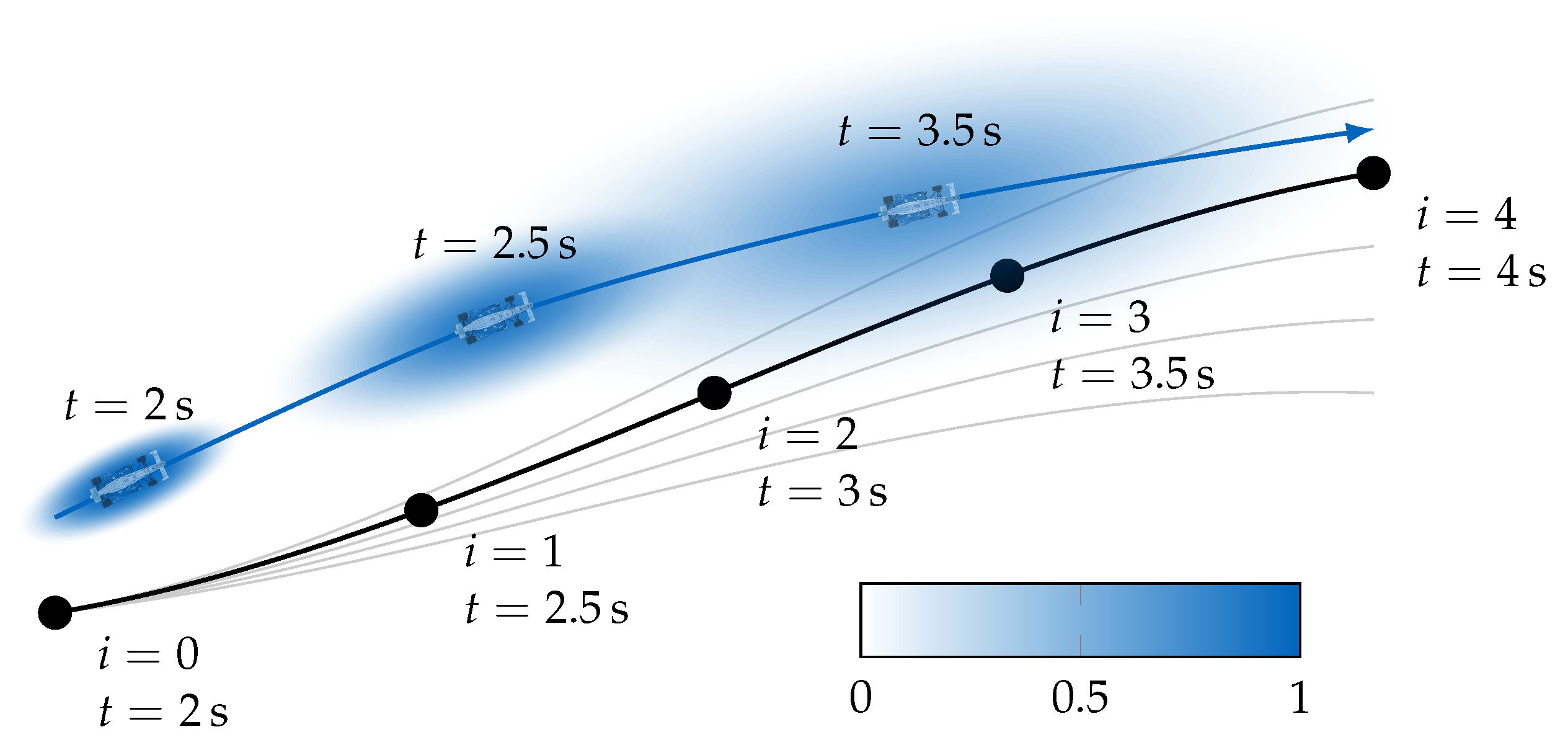
Each term is a product of a weight w and a feature of the edge at the discretization point. They cause different, sometimes contradictory, behaviors. On the one hand, the vehicle should reach a high velocity and follow the racing line to achieve a minimum lap time. On the other hand, it has to deviate from the racing line to overtake other vehicles and slow down if necessary. The Euclidean distance d rl to the offline-generated optimal racing line causes the vehicle to follow the racing line whenever possible. The linear contribution of d rl , instead of d rl 2 , allows the vehicle to follow the racing line in single-vehicle scenarios but leaves enough incentive to deviate from it during overtaking maneuvers. The second term penalizes the deviation from the target velocity v d given either by the racing line or by race rules. The third term penalizes the curvature κ to avoid abrupt steering at high velocities. For scenarios with static and dynamic obstacles, the last term takes into account the prediction to maintain a sufficient distance to the obstacles and to perform overtaking maneuvers. The prediction cost depends on the longitudinal and lateral distances of the predicted vehicle to the discretization point i and a time-dependent factor g ( t ) . It is computed using Equation (5), where d x , i and d y , i are the longitudinal and lateral distances in the local coordinate system of the predicted vehicle:
d pred , i = max 1 1 d x , max 2 ( t ) 1 d y , max 2 ( t ) T d x , i 2 d y , i 2 , 0 g ( t )
The elliptical shape of d pred , i is illustrated for three discretization points along an exemplary edge in Figure 4. The cost increases to a maximum value of 1 as the position of a discretization point approaches the predicted vehicle’s center. d x , max ( t ) and d y , max ( t ) specify at which longitudinal and lateral distances the prediction costs are incurred so that the values of these parameters can easily be set according to the desired safety distances. The choice of d x , max ( t ) > d y , max ( t ) reflects the more uncertain predicted longitudinal movement. Furthermore, d x , max ( t ) and d y , max ( t ) increase as the time horizon progresses to account for less certain predictions further in the future. However, too-wide ellipses can lead to conservative behaviors, i.e., just following a vehicle instead of overtaking it, since all accelerating edges across the entire width of the race track come within the range of the ellipses. If the velocity cost is not weighted high enough, it is better to stay behind a vehicle to avoid entering the expensive area covered by ellipses. To mitigate this problem, the factor g ( t ) decreases linearly with time so that the prediction and velocity cost terms are of similar magnitude, allowing a planned overtaking maneuver that maximizes the lateral distance to the vehicle ahead.
The described interacting influences of the velocity and prediction costs and other conflicting behaviors illustrate the importance of a proper distribution of the weights w rl , w v , w κ , w pred , and the other parameters. Different parameter sets are selected depending on the environment (pit lane or race track) and the race condition. Since d x , max ( t ) and d y , max ( t ) have a physical interpretation they can be set according to the required safety distances given by the race rules. The weights, however, are more difficult to tune. In our case, empirically determined values were used so that the racing line was followed in single driving scenarios, but the prediction costs dominated in the presence of obstacles. For more general behaviors, the tuning could be automated by optimizing the weights based on a collection of safety-critical and performance-oriented scenarios.

3. Results and Discussion

In the following, we present results from the racing event Autonomous Challenge at CES (AC@CES) at the LVMS on 7 January 2022 [44]. The proposed planning approach was integrated into the sequential software architecture of TUM Autonomous Motorsports in Figure 5. The used full-scale prototype Dallara AV-21 in Figure 1 had an eight-core Intel Xeon E-2278GE CPU with 3.3   G Hz and 64 GB RAM. Our chosen allocation of computing resources to the individual modules left one CPU core available for the local planning approach. The final trajectory should reach a minimal planning horizon of 5 s . The software architecture met all requirements listed in Section 2.1 with the tracking controller in [45], which was based on a Tube-MPC approach, and the racing line generation in [13]. The sampling procedure used to generate the initial edges is described in [46]. Similar to [24,25], it was based on the generation of jerk-minimal trajectories but only constituted the first part of the final trajectory. The longitudinal distance of the layers was 75 m and the lateral spacing of the nodes was 1.4   m . The sampling procedure and the proposed graph search were written in Python 3.8 , while some functions used Numpy or were written in C.
The race rules at the AC@CES prescribe alternating overtaking maneuvers. The leading vehicle, the defender, has to maintain a fixed velocity and stay on the inner (left) side of the race track. The following vehicle, the attacker, has to complete an overtaking maneuver within a specified passing zone. After a successful overtaking maneuver, the roles switch. If both competitors successfully overtake, the defender’s velocity increases, and the race’s next round begins. For this form of competition, our offline-generated racing line was restricted to the inner side of the track to make the defender behavior the default behavior. Furthermore, the inner racing line encouraged natural overtaking maneuvers, where the swerve to initiate the maneuver and the switch back to the inside solely resulted from the edge costs. In the final event, our software was able to perform overtaking maneuvers with attacker velocities of up to 74 m/s. The following sections focus on the two fastest overtaking maneuvers to illustrate the behavioral planning and advantages of the UCS over an exhaustive search for a long planning horizon. A video of the corresponding race section can be found at https://youtu.be/XUIctOJdrLk (accessed on 2 November 2022).

3.1. Overtaking Maneuver

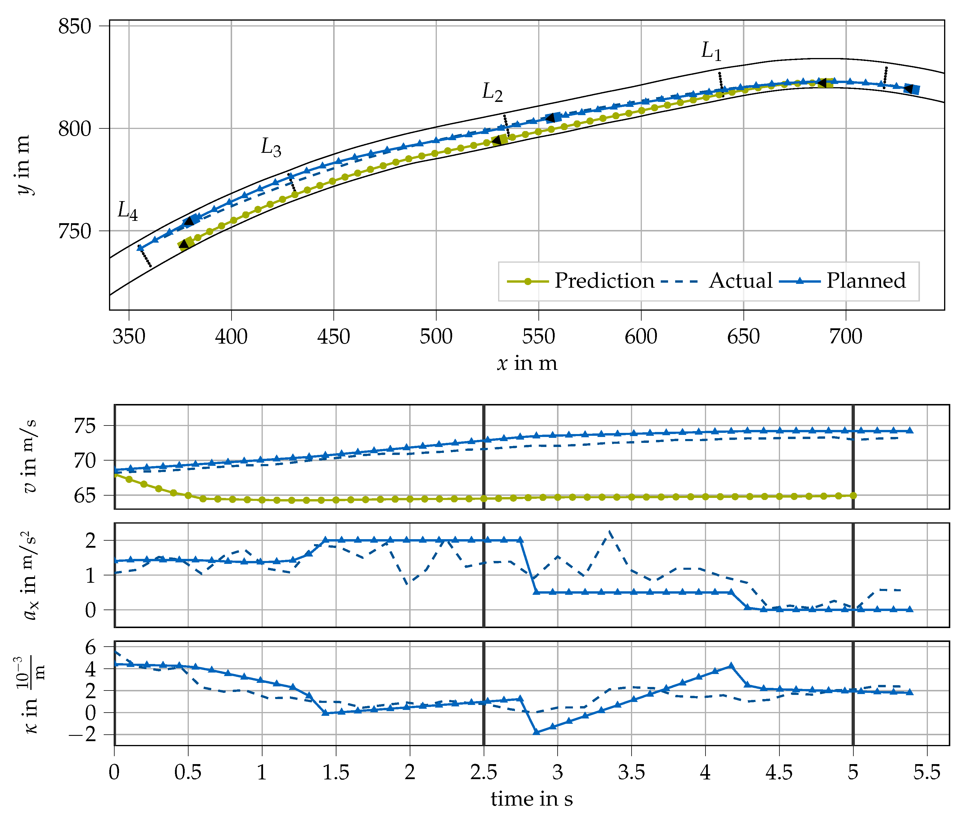
Figure 6 shows the fastest achieved attacker scenario after entering the passing zone. In the selected planning step, in the following called planning step ⓓ, the sampling procedure reached layer L 1 and the graph search proceeded for three layers. The last edge of the final trajectory to layer L 4 reached a time of 5.4   s , satisfying the minimum planning horizon of 5 s . While the planned velocity profile was continuous, the acceleration and curvature profiles showed the expected discontinuities at the layers, which illustrated the behavioral nature of the graph search result. The result of planning step ⓓcould be interpreted as a maneuver to accelerate and overtake the defender on the right side. The subsequent Tube-MPC reoptimized the coarse trajectory so that the tracked acceleration and curvature profiles were smoother. With the chosen discretization for the sampled constant accelerations between two layers, it was possible to accelerate at 2 m/s 2 between L 1 and L 2 and at 0.5 m/s between L 2 and L 3 . With these limits, it took 5 s for the attacker to be side-by-side with the defender, emphasizing the need for a long planning horizon.
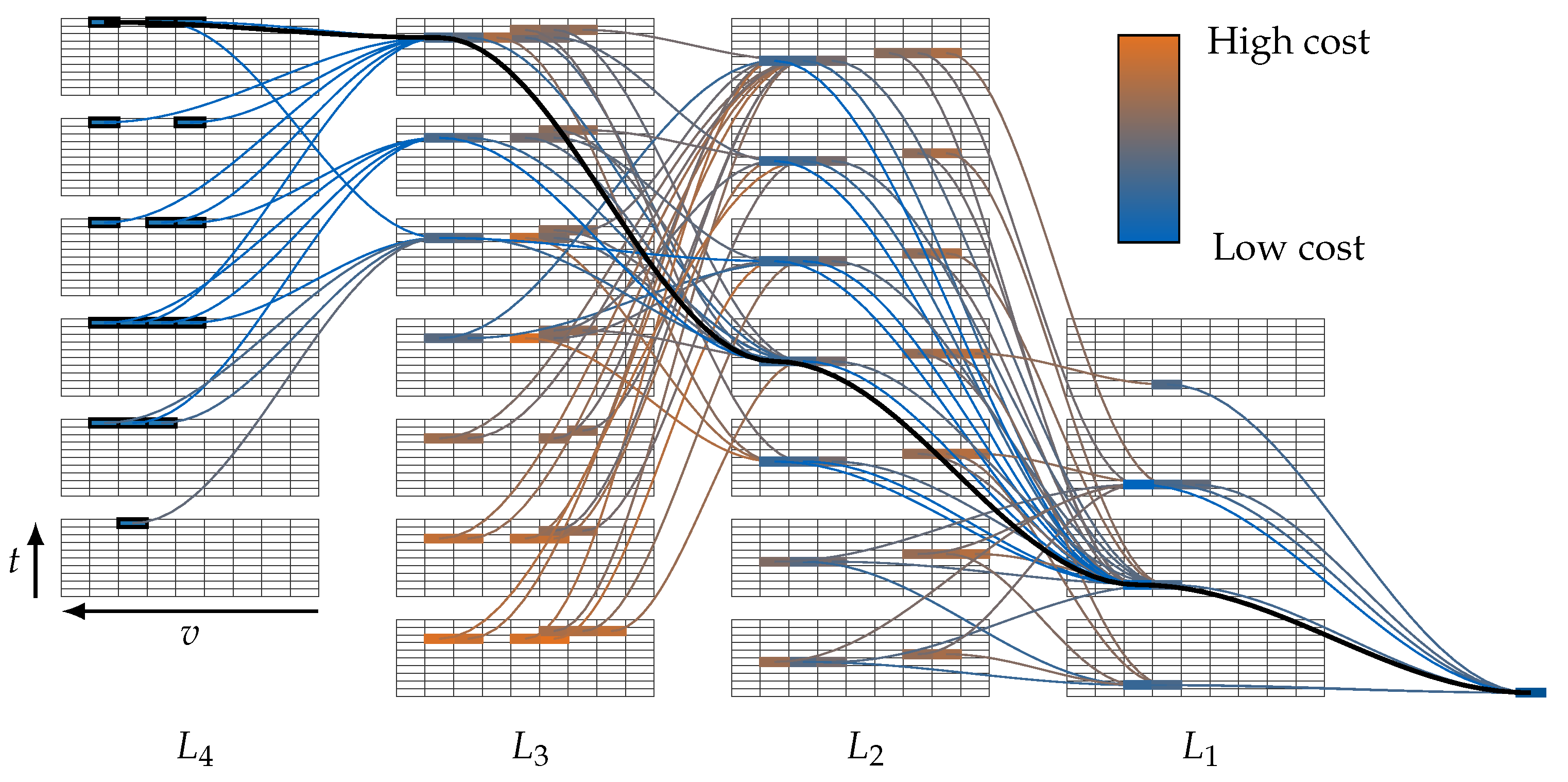
Figure 7 illustrates the generated spatiotemporal graph for planning step ⓓ. Edges lying on the inside of the race track came into the range of the prediction cost ellipses and thus received high costs. The prediction costs dominated the racing line costs, so deviating from the racing line and keeping a high velocity was better than staying inside behind the defender. Although the prediction cost was not incurred until the latter part of the planning horizon, it gave an incentive to deviate from the racing line early at layer L 1 since in the long term the inside paths would end up in the high-cost region. Due to the wide prediction cost ellipses near the end of the planning horizon, the planned trajectory kept a maximum lateral distance, as can also be seen in Figure 6. This and the early reaction were advantageous in terms of recursive feasibility so that overtaking solutions could still be found in later planning steps.
Due to the high prediction costs on the inside, the UCS did not explore this region further. Similarly, the velocity costs contributed to the reduction in the number of edges since nodes with high velocities were expanded first, more likely leading to the optimal path. In the planning step ⓓ, the UCS could reduce the number of generated edges from 2544 to 409 compared to the exhaustive search and found 15 suboptimal goal nodes, all of them located in layer L 4 . The suboptimal goal nodes were mainly reached by decelerating edges.
Figure 6 and Figure 7 also highlight the multistep characteristic of our approach. As illustrated in Figure 7, it was planned to change the lateral position until layer L 3 and maintain a constant lateral distance to the track boundaries from layer L 3 to L 4 . The acceleration profile in Figure 6 shows that the vehicle accelerated until layer L 3 and maintained the velocity from layer L 3 to L 4 . Since the approaches in [24,25,46] sampled time, velocity, and lateral displacement for only one step, the resulting trajectories could not represent the described maneuver. However, a drawback of our approach compared to the jerk-minimal one-step approaches arises from the constant acceleration between two layers. In Equation (2), a x remains constant by design, a x , max ( v ) , a y , max ( v ) , and a y , however, vary depending on the velocity and track geometry. Especially on oval race tracks, the distance between two layers can be large, so the spatiotemporal edges can cover a large velocity range. While driving at the limits, this can generate many infeasible edges, and only edges that keep the current velocity remain. The variable accelerations of the jerk-minimal trajectories in [24,25] show better-suited profiles for high velocities, so fewer edges are sorted out and driving closer to the limits is possible. Therefore, we followed the jerk-minimal approach for the sampling procedure.

3.2. Comparison of the Search Methods

Reducing the number of generated edges directly affected the computation time. Figure 8 depicts the computation times for the two fastest overtaking maneuvers and one defender scenario obtained by recalculations on comparable hardware. The computation time of the sampling procedure is included and was approximately constant at 10 m s . Considering fewer edges by the UCS resulted in shorter and more consistent computation times compared to the exhaustive search. The large fluctuations in the computation time of the exhaustive search resulted from the alternating straight and curved track sections. In general, more edges were generated on straight sections since many edges failed the feasibility checks in turns at high velocities. In contrast to the exhaustive search, the computation time for each planning step using the UCS stayed below the upper limit of t thr   = 300   m s . This means that the search could always be terminated early when the optimal solution was found. The average computation time of the exhaustive search was 345 m s , while the UCS undercut the target of 150 m s with an average computation time of 99 m s in the presented race section. Compared to the recent sampling approach in [25], the computation time was larger, and the GPU performance reported in [27] for the exhaustive search could not be achieved. However, for the given use case, it was sufficient and enabled the exploration of more maneuvers with a longer planning horizon.
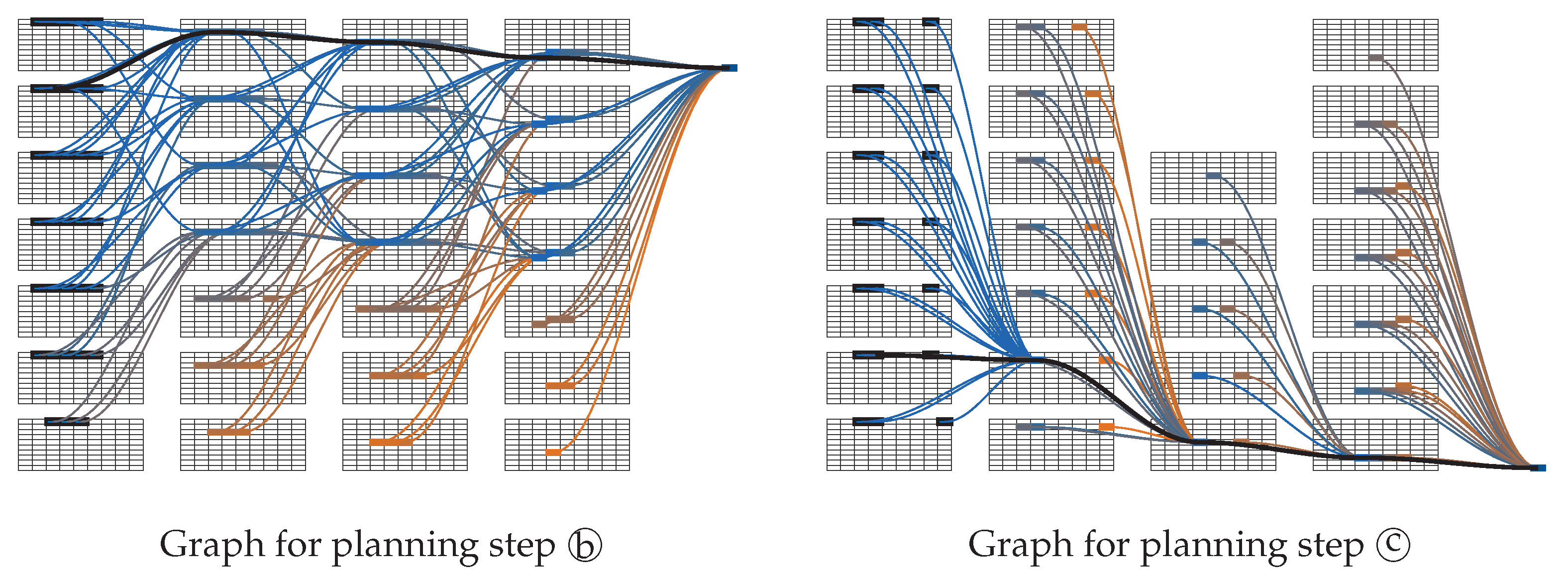
An increased computation time was observed during the overtaking maneuvers in the role of an attacker. This increase could be explained by the deviation from the racing line during the overtaking process. Nodes close to the racing line were expanded first, but then, the reached nodes were not expanded due to the high prediction cost resulting in high costs-to-come. As a defender, on the other hand, the costs along the racing line were the lowest, so that significantly fewer iterations through the frontier (Line 6 in Algorithm 1) took place until the optimal path was found. This was also why the computation time of the UCS was not influenced by straight or curved track sections. The resulting graphs are compared in Figure 9. A peak in computation time can be observed for planning step ⓐ. Here, the UCS reached the computation time of the exhaustive search. In this planning step, a falsely detected vehicle with low velocity in a no-passing zone caused all edges to have similar costs. Hence, the phenomenon described at the end of Section 2.4.2 came into play, and the UCS expanded the nodes in an order nearly identical to the exhaustive search.
With regard to the suboptimal goal nodes, further analyses showed that the first suboptimal goal node was found after 60% to 80% of the iterations through the frontier needed to find the optimal solution. Moreover, as can be seen in Figure 7 and Figure 9, most of the suboptimal goal nodes were reached with a smaller velocity than the final goal node resulting in defensive braking maneuvers in the case of early search terminations.

4. Conclusions and Outlook

We presented a graph-search-based planning approach capable of generating trajectories for racing on an oval race track. Searching in a discretized spatiotemporal state space finds a trajectory that represents the optimal behavior in the presence of a predicted competitor. Despite a long planning horizon and many maneuver variants, we achieved computation times sufficient for the presented use case. This was accomplished by the specific graph structure with intervals for the velocity and time dimensions and by the efficient graph search algorithm. Furthermore, our proposed cost function, if properly parameterized, could generate a competitive behavior with early reactions to obstacles due to the long planning horizon, allowing a safe operation at high velocities. The proposed mechanism for a suboptimal solution did not need to be applied in the presented scenario but worked successfully in simulations and will be analyzed in future work. The resulting behaviors are of particular interest.
The total computation time should be further reduced for races with more competitors, complex scenarios, and hence more uncertain predictions. Our approach could be implemented in C and partly parallelized if sufficient resources were available. However, the computation time benefit would be less than in [27], since the UCS only allows a parallelization at a node expansion level while the exhaustive search can be parallelized at a layer level.
Besides racing, the presented search method could be applied in traffic scenarios as initially proposed for the given graph in [27]. Instead of the racing line, a lanelet network could provide the reference for the cost function. However, a traffic scenario would require additional terms and a behavior state machine to consider traffic rules and meet comfort goals. Both racing and traffic scenarios include highly interactive scenarios, which have been neglected in this work. Future work will analyze how the cost function of general sampling and search-based planning approaches can consider mutual influence.

Author Contributions

Conceptualization, M.R. and L.Ö.; methodology, M.R., L.Ö. and T.K.; software, M.R., L.Ö. and T.K.; validation, M.R.; formal analysis, M.R. and T.K.; investigation, M.R. and L.Ö.; data curation, M.R. and T.K.; writing—original draft preparation, M.R.; writing—review and editing, M.R., L.Ö., T.K. and B.L.; visualization, M.R.; supervision, B.L. All authors have read and agreed to the published version of the manuscript.

Funding

This research received no external funding.

Data Availability Statement

The data presented in this study are available on reasonable request.

Acknowledgments

We want to thank the entire team of TUM Autonomous Motorsports for enabling us to execute our planning approach on a full-scale prototype successfully. We thank the organizers of the Indy Autonomous Challenge (IAC), Juncos Hollinger Racing, and all participating teams who made the IAC possible. Furthermore, we thank Saskia Brose, Thomas Herrmann, and Tim Stahl for their experienced inputs and revisions.

Conflicts of Interest

The authors declare no conflict of interest.

Abbreviations

The following abbreviations are used in this manuscript:
LVMSLas Vegas Motor Speedway
IMSIndianapolis Motor Speedway
IACIndy Autonomous Challenge
AC@CESAutonomous Challenge at CES
RRTRapidly exploring random trees
UCSUniform-cost search
TUMTechnical University of Munich
MPCModel predictive control
OCPOptimal control problem
NLPNonlinear programming
PVDPath-velocity decomposition

References

  1. Buehler, M.; Iagnemma, K.; Singh, S. (Eds.) The 2005 DARPA Grand Challenge; Springer Tracts in Advanced Robotics; Springer: Berlin/Heidelberg, Germany, 2007; Volume 36. [Google Scholar] [CrossRef]
  2. Buehler, M.; Iagnemma, K.; Singh, S. (Eds.) The DARPA Urban Challenge; Springer Tracts in Advanced Robotics; Springer: Berlin/Heidelberg, Germany, 2009; Volume 56. [Google Scholar] [CrossRef]
  3. Theodosis, P.A.; Gerdes, J.C. Nonlinear Optimization of a Racing Line for an Autonomous Racecar Using Professional Driving Techniques. In Proceedings of the ASME 5th Annual Dynamic Systems and Control Division Conference and JSME 11th Motion and Vibration Conference, Fort Lauderdale, FL, USA, 17–19 October 2012; ASME: New York, NY, USA, 2013; pp. 235–241. [Google Scholar] [CrossRef]
  4. Heilmeier, A.; Wischnewski, A.; Hermansdorfer, L.; Betz, J.; Lienkamp, M.; Lohmann, B. Minimum curvature trajectory planning and control for an autonomous race car. Veh. Syst. Dyn. 2020, 58, 1497–1527. [Google Scholar] [CrossRef]
  5. Roborace. Available online: https://roborace.com/ (accessed on 2 November 2022).
  6. Kant, K.; Zucker, S.W. Toward Efficient Trajectory Planning: The Path-Velocity Decomposition. Int. J. Robot. Res. 1986, 5, 72–89. [Google Scholar] [CrossRef]
  7. Paden, B.; Cap, M.; Yong, S.Z.; Yershov, D.; Frazzoli, E. A Survey of Motion Planning and Control Techniques for Self-Driving Urban Vehicles. IEEE Trans. Intell. Veh. 2016, 1, 33–55. [Google Scholar] [CrossRef] [Green Version]
  8. Ziegler, J.; Bender, P.; Dang, T.; Stiller, C. Trajectory Planning for Bertha—A Local, Continuous Method. In Proceedings of the 2014 IEEE Intelligent Vehicles Symposium Proceedings, Dearborn, MI, USA, 8–11 June 2014; IEEE: Piscataway, NJ, USA, 2014; pp. 450–457. [Google Scholar] [CrossRef]
  9. Cremean, L.B.; Foote, T.B.; Gillula, J.H.; Hines, G.H.; Kogan, D.; Kriechbaum, K.L.; Lamb, J.C.; Leibs, J.; Lindzey, L.; Rasmussen, C.E.; et al. Alice: An Information-Rich Autonomous Vehicle for High-Speed Desert Navigation. In The 2005 DARPA Grand Challenge; Springer Tracts in Advanced Robotics; Buehler, M., Iagnemma, K., Singh, S., Eds.; Springer: Berlin/Heidelberg, Germany, 2007; Volume 36, pp. 437–482. [Google Scholar] [CrossRef]
  10. Veneri, M.; Massaro, M. A free-trajectory quasi-steady-state optimal-control method for minimum lap-time of race vehicles. Veh. Syst. Dyn. 2020, 58, 933–954. [Google Scholar] [CrossRef]
  11. Lovato, S.; Massaro, M. A three-dimensional free-trajectory quasi-steady-state optimal-control method for minimum-lap-time of race vehicles. Veh. Syst. Dyn. 2022, 60, 1512–1530. [Google Scholar] [CrossRef]
  12. Casanova, D. On Minimum Time Vehicle Manoeuvring: The Theoretical Optimal Lap. Ph.D. Thesis, Cranfield University, Silsoe, UK, 2000. [Google Scholar]
  13. Christ, F.; Wischnewski, A.; Heilmeier, A.; Lohmann, B. Time-optimal trajectory planning for a race car considering variable tyre-road friction coefficients. Veh. Syst. Dyn. 2021, 59, 588–612. [Google Scholar] [CrossRef]
  14. Gundlach, I.; Konigorski, U. Modellbasierte Online-Trajektorienplanung für zeitoptimale Rennlinien. Automatisierungstechnik 2019, 67, 799–813. [Google Scholar] [CrossRef]
  15. Subosits, J.K.; Gerdes, J.C. From the Racetrack to the Road: Real-Time Trajectory Replanning for Autonomous Driving. IEEE Trans. Intell. Veh. 2019, 4, 309–320. [Google Scholar] [CrossRef]
  16. Zhu, Z.; Schmerling, E.; Pavone, M. A Convex Optimization Approach to Smooth Trajectories for Motion Planning with Car-Like Robots. In Proceedings of the 2015 54th IEEE Conference on Decision and Control (CDC), Osaka, Japan, 15–18 December 2015; IEEE: Piscataway, NJ, USA, 2015; pp. 835–842. [Google Scholar] [CrossRef] [Green Version]
  17. Xin, L.; Kong, Y.; Li, S.E.; Chen, J.; Guan, Y.; Tomizuka, M.; Cheng, B. Enable faster and smoother spatio-temporal trajectory planning for autonomous vehicles in constrained dynamic environment. Proc. Inst. Mech. Eng. Part D J. Automob. Eng. 2021, 235, 1101–1112. [Google Scholar] [CrossRef]
  18. Liniger, A.; Domahidi, A.; Morari, M. Optimization-based autonomous racing of 1:43 scale RC cars. Optim. Control. Appl. Methods 2015, 36, 628–647. [Google Scholar] [CrossRef] [Green Version]
  19. Svensson, L.; Bujarbaruah, M.; Kapania, N.R.; Torngren, M. Adaptive Trajectory Planning and Optimization at Limits of Handling. In Proceedings of the 2019 IEEE/RSJ International Conference on Intelligent Robots and Systems (IROS), Macau, China, 3–8 November 2019; IEEE: Piscataway, NJ, USA, 2019; pp. 3942–3948. [Google Scholar] [CrossRef] [Green Version]
  20. Bender, P.; Tas, O.S.; Ziegler, J.; Stiller, C. The Combinatorial Aspect of Motion Planning: Maneuver Variants in Structured Environments. In Proceedings of the 2015 IEEE Intelligent Vehicles Symposium (IV), Seoul, Korea, 28 June–1 July 2015; IEEE: Piscataway, NJ, USA, 2015; pp. 1386–1392. [Google Scholar] [CrossRef]
  21. Li, B.; Yin, Z.; Ouyang, Y.; Zhang, Y.; Zhong, X.; Tang, S. Online Trajectory Replanning for Sudden Environmental Changes during Automated Parking: A Parallel Stitching Method. IEEE Trans. Intell. Veh. 2022, 7, 748–757. [Google Scholar] [CrossRef]
  22. He, S.; Zeng, J.; Sreenath, K. Autonomous Racing with Multiple Vehicles using a Parallelized Optimization with Safety Guarantee using Control Barrier Functions. In Proceedings of the 2022 International Conference on Robotics and Automation (ICRA), Philadelphia, PA, USA, 23–27 May 2022; IEEE: Piscataway, NJ, USA, 2022; pp. 3444–3451. [Google Scholar] [CrossRef]
  23. Stahl, T.; Wischnewski, A.; Betz, J.; Lienkamp, M. Multilayer Graph-Based Trajectory Planning for Race Vehicles in Dynamic Scenarios. In Proceedings of the 2019 IEEE Intelligent Transportation Systems Conference (ITSC), Auckland, New Zealand, 27–30 October 2019; IEEE: Piscataway, NJ, USA, 2019; pp. 3149–3154. [Google Scholar] [CrossRef]
  24. Werling, M.; Ziegler, J.; Kammel, S.; Thrun, S. Optimal Trajectory Generation for Dynamic Street Scenarios in a Frenét Frame. In Proceedings of the 2010 IEEE International Conference on Robotics and Automation, Anchorage, AK, USA, 3–7 May 2010; IEEE: Piscataway, NJ, USA, 2010; pp. 987–993. [Google Scholar] [CrossRef]
  25. Raji, A.; Liniger, A.; Giove, A.; Toschi, A.; Musiu, N.; Morra, D.; Verucchi, M.; Caporale, D.; Bertogna, M. Motion Planning and Control for Multi Vehicle Autonomous Racing at High Speeds. In Proceedings of the 2022 IEEE International Conference on Intelligent Transportation Systems (IEEE ITSC 2022), Macau, China, 8–12 October 2022; IEEE: Piscataway, NJ, USA, 2022. [Google Scholar]
  26. Ziegler, J.; Stiller, C. Spatiotemporal state lattices for fast trajectory planning in dynamic on-road driving scenarios. In Proceedings of the 2009 IEEE/RSJ International Conference on Intelligent Robots and Systems, St. Louis, MO, USA, 10–15 October 2009; IEEE: Piscataway, NJ, USA, 2009; pp. 1879–1884. [Google Scholar] [CrossRef]
  27. McNaughton, M.; Urmson, C.; Dolan, J.M.; Lee, J.W. Motion Planning for Autonomous Driving with a Conformal Spatiotemporal Lattice. In Proceedings of the 2011 IEEE International Conference on Robotics and Automation, Shanghai, China, 9–13 May 2011; IEEE: Piscataway, NJ, USA, 2011; pp. 4889–4895. [Google Scholar] [CrossRef]
  28. Morsali, M.; Frisk, E.; Aslund, J. Spatio-Temporal Planning in Multi-Vehicle Scenarios for Autonomous Vehicle Using Support Vector Machines. IEEE Trans. Intell. Veh. 2021, 6, 611–621. [Google Scholar] [CrossRef]
  29. LaValle, S.M. Rapidly-Exploring Random Trees: A New Tool for Path Planning. Technical Report 98-11; Iowa State University, Department of Computer Science: Ames, IA, USA, 1998. [Google Scholar]
  30. Arslan, O.; Berntorp, K.; Tsiotras, P. Sampling-based Algorithms for Optimal Motion Planning Using Closed-loop Prediction. In Proceedings of the 2017 IEEE International Conference on Robotics and Automation (ICRA), Singapore, 29 May–3 June 2017; IEEE: Piscataway, NJ, USA, 2017; pp. 4991–4996. [Google Scholar] [CrossRef] [Green Version]
  31. Feraco, S.; Luciani, S.; Bonfitto, A.; Amati, N.; Tonoli, A. A local trajectory planning and control method for autonomous vehicles based on the RRT algorithm. In Proceedings of the 2020 AEIT International Conference of Electrical and Electronic Technologies for Automotive (AEIT AUTOMOTIVE), Turin, Italy, 18–20 November 2020; IEEE: Piscataway, NJ, USA, 2020; pp. 1–6. [Google Scholar] [CrossRef]
  32. Liniger, A.; Lygeros, J. A Viability Approach for Fast Recursive Feasible Finite Horizon Path Planning of Autonomous RC Cars. In Proceedings of the 18th International Conference on Hybrid Systems: Computation and Control, Seattle, WA, USA, 14–16 April 2015; Girard, A., Sankaranarayanan, S., Eds.; ACM: New York, NY, USA, 2015; pp. 1–10. [Google Scholar] [CrossRef]
  33. Liniger, A.; Lygeros, J. A Noncooperative Game Approach to Autonomous Racing. IEEE Trans. Control. Syst. Technol. 2020, 28, 884–897. [Google Scholar] [CrossRef] [Green Version]
  34. Wang, M.; Wang, Z.; Talbot, J.; Gerdes, J.C.; Schwager, M. Game-Theoretic Planning for Self-Driving Cars in Multivehicle Competitive Scenarios. IEEE Trans. Robot. 2021, 37, 1313–1325. [Google Scholar] [CrossRef]
  35. Bahram, M.; Lawitzky, A.; Friedrichs, J.; Aeberhard, M.; Wollherr, D. A Game-Theoretic Approach to Replanning-Aware Interactive Scene Prediction and Planning. IEEE Trans. Veh. Technol. 2016, 65, 3981–3992. [Google Scholar] [CrossRef]
  36. Fisac, J.F.; Bronstein, E.; Stefansson, E.; Sadigh, D.; Sastry, S.S.; Dragan, A.D. Hierarchical Game-Theoretic Planning for Autonomous Vehicles. In Proceedings of the 2019 International Conference on Robotics and Automation (ICRA), Montreal, QC, Canada, 20–24 May 2019; IEEE: Piscataway, NJ, USA, 2019; pp. 9590–9596. [Google Scholar] [CrossRef] [Green Version]
  37. Bellman, R. Dynamic Programming; Princeton University Press: Princeton, NJ, USA, 1957. [Google Scholar]
  38. Hermansdorfer, L.; Betz, J.; Lienkamp, M. Benchmarking of a software stack for autonomous racing against a professional human race driver. In Proceedings of the 2020 Fifteenth International Conference on Ecological Vehicles and Renewable Energies (EVER), Monte-Carlo, Monaco, 10–12 September 2020; IEEE: Piscataway, NJ, USA, 2020; pp. 1–8. [Google Scholar] [CrossRef]
  39. Herrmann, T.; Wischnewski, A.; Hermansdorfer, L.; Betz, J.; Lienkamp, M. Real-Time Adaptive Velocity Optimization for Autonomous Electric Cars at the Limits of Handling. IEEE Trans. Intell. Veh. 2021, 6, 665–677. [Google Scholar] [CrossRef]
  40. Betz, J.; Betz, T.; Fent, F.; Geisslinger, M.; Heilmeier, A.; Hermansdorfer, L.; Herrmann, T.; Huch, S.; Karle, P.; Lienkamp, M.; et al. TUM Autonomous Motorsport: An Autonomous Racing Software for the Indy Autonomous Challenge. arXiv 2022, arXiv:2205.15979. [Google Scholar] [CrossRef]
  41. Dijkstra, E.W. A Note on Two Problems in Connexion with Graphs. Numer. Math. 1959, 1, 269–271. [Google Scholar] [CrossRef] [Green Version]
  42. Felner, A. Position Paper: Dijkstra’s Algorithm versus Uniform Cost Search or a Case Against Dijkstra’s Algorithm. In Proceedings of the The Fourth International Symposium on Combinatorial Search (SoCS-2011), Barcelona, Spain, 15–16 July 2011; pp. 47–51. [Google Scholar]
  43. Russell, S.J.; Norvig, P. Artificial Intelligence: A Modern Approach, 3rd ed.; Prentice Hall: Upper Saddle River, NJ, USA, 2010. [Google Scholar]
  44. Indy Autonomous Challenge. Available online: https://www.indyautonomouschallenge.com/ (accessed on 2 November 2022).
  45. Wischnewski, A.; Herrmann, T.; Werner, F.; Lohmann, B. A Tube-MPC Approach to Autonomous Multi-Vehicle Racing on High-Speed Ovals. IEEE Trans. Intell. Veh. 2022, 1. [Google Scholar] [CrossRef]
  46. Ögretmen, L.; Rowold, M.; Ochsenius, M.; Lohmann, B. Smooth Trajectory Planning at the Handling Limits for Oval Racing. Actuators, 2022; accepted. [Google Scholar]
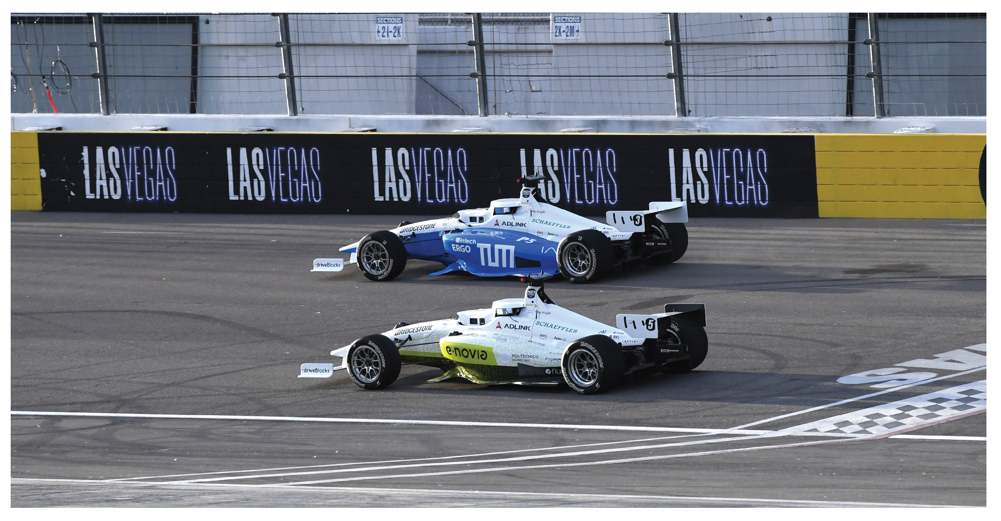
Figure 1. Dallara AV-21: Full-scale prototype of TUM Autonomous Motorsports (back) running the proposed planning algorithm at the LVMS and overtaking a dynamic obstacle.
Actuators 11 00319 g001
Figure 2. Spatial graph. The layers group spatial nodes. Spatial edges connect the spatial nodes and represent available paths.
Actuators 11 00319 g002
Figure 3. Spatiotemporal graph. The sampling procedure connects the initial state with the spatiotemporal state lattice. A graph search follows, starting at the connected nodes (here, only shown for one node).
Actuators 11 00319 g003
Figure 4. Prediction cost. The considered edge, shown in black, is discretized with five points and covers the time range from t = 2   s to t = 4   s . The predicted path is shown in blue, together with the ellipses for the discretization points i = 0 , 1 , 3 . The point i = 3 is covered by the corresponding ellipses so that the prediction cost of this edge is nonzero.
Actuators 11 00319 g004
Figure 5. Software architecture: the software of TUM Autonomous Motorsports follows a sequential approach.
Actuators 11 00319 g005
Figure 6. Initiation of an overtaking maneuver in planning step ⓓ. The planned and actually driven path, velocity, acceleration, and curvature are shown in blue. The correctly predicted path and velocity of the defender are green. The planned and predicted poses of the vehicles are shown for t = 0 and the times marked by the vertical lines in the lower plots.
Actuators 11 00319 g006
Figure 7. Generated graph for planning step ⓓ. Only the relevant spatial nodes and edges that contribute to an optimal path to reach a spatiotemporal node are shown for a clearer picture. The reached nodes are qualitatively colored according to their cost-to-come and the edges according to their cost. The optimal path is shown in black, and all nodes satisfying the goal condition are outlined in black.
Actuators 11 00319 g007
Figure 8. Comparison of computation times. The planning steps of the considered race section were recalculated with the UCS and the exhaustive search. The black-dotted line shows the actual computation times for the UCS on Dallara AV-21 hardware during the race. The defending and attacking maneuvers are highlighted.
Actuators 11 00319 g008
Figure 9. Comparison of graphs for defending and attacking scenarios: 450 edges were generated while overtaking in planning step ⓑ and 162 edges were generated while being overtaken in planning step ⓒ. The colors and grids are defined analogously to Figure 7.
Actuators 11 00319 g009
Publisher’s Note: MDPI stays neutral with regard to jurisdictional claims in published maps and institutional affiliations.