A Variable Stiffness Actuator Based on Leaf Springs: Design, Model and Analysis

Abstract

In order to adapt to complex and changeable mechanical conditions and make the deformable mechanisms perform well statically and dynamically, variable stiffness joints have been studied extensively. The variable stiffness actuator is the key driving component to adjust stiffness of the joint. By inserting flexible elements between the driving and driven ends of rigid motion, the variable stiffness actuator makes the joint move precisely and allows humans to interact with machines safely. At present, many kinds of variable stiffness actuators have been applied, among which the way of changing the length of the force arm of leaf springs has obvious advantages. However, overall configuration design, accurate stiffness model, mechanical characteristics and safety analysis have not been studied in depth. This paper investigates a variable stiffness actuator based on leaf spring by design, model and mechanical analysis. The composition and configuration of the actuator is analyzed and optimized. Using the deflection theory of the beam, a new rotational stiffness model of the actuator is established, and a safe position criterion is set up upon the deformation constraint conditions. The variation law of stiffness and the influence of parameters on mechanical characteristics are studied. The finite element analysis method verified the rotational stiffness model, and static test proved that the actuator could effectively work in the joint.

1. Introduction

In recent years, the demands for smart manufacturing and improved quality of life have gradually increased. Therefore, researchers have devoted themselves to studying deformable mechanisms that can adapt to complex mechanical environments. These mechanisms include multi-joint robots, large-scale foldable mechanisms, and morphing drafts, among others. A joint is the structural foundation of deformable mechanisms, and its stiffness is an important factor affecting the static and dynamic characteristics of mechanisms [1,2,3]. Traditional rigid joints can bear a high load, respond quickly and locate accurately, but usually produce violent impacts instantly, which is unsafe for the system [4]. In comparison, low stiffness can reduce the reaction moment and mitigate impact. However, it is easy to produce a steady-state oscillation [5]. To make the mechanisms adapt to a changeable environment, research on variable stiffness joints is increasing. A variable stiffness actuator is an important component to adjust the stiffness of a joint. Its function is to transfer flexible motion by adding elements with adjustable flexibility at the driving shaft and the driven shaft of the joint. Therefore, variable stiffness actuators that meet these requirements require that variable stiffness joints improve bearing capacity, increase the variation range of stiffness and become smaller. In addition, they also provide important technical support for the development of deformable mechanisms that are lightweight, intelligent and have secure human-computer interactions.

According to the transmission principle, the actuating mechanism of a variable stiffness actuator includes a variable elastic force, an adjustable non-contact force, the interface force of the material, and intelligent materials. Variable stiffness actuators have been widely used in compliant robots, bionic soft grippers, and intelligent space mechanisms. For example: (1) With respect to magnetic force, if the distance between the two magnets or the current inside an exciting coil is adjusted, the magnetic force changes so that the ability to transmit torque can be adjusted and the stiffness changes [6,7]. (2) With respect to pneumatic force, a sealed cavity with the desired shape is manufactured using rubber material, and stiffness is varied by changing the air pressure inside [8,9,10,11]. (3) For interfacial force [12], the force of interlocking bristles [13] and particle friction [14,15] can directly affect the transmission property and the force between the interfaces, thus changing the transmission stiffness. (4) With respect to smart materials, under the action of external excitation such as electricity, magnetism and heat, some special materials change phases or macroscopic structures. Based on this mechanism, smart materials, such as shape memory alloys [16], liquid metals [17], dielectric high-elasticity polymers [18], electrorheological fluids [19,20,21,22] and magnetorheological fluids [23], have been applied to variable stiffness joints in recent years. (5) With respect to electrohydrodynamics (EHD) an EHD pump [24,25] can easily and quickly control the flow direction of a dielectric liquid by changing the voltage, and then drive a soft structure to change stiffness to perform bending, twisting and stretching movements. (6) With respect to variable elastic force, elastic elements such as torsion springs [26,27,28] and linear springs [29] can be installed between the input and output of a rigid transmission path, and the transmission stiffness varied by changing the length of the force arm [30] or the preload force [31]. Among elastic elements used in variable stiffness actuators, a leaf spring is a special element. To some extent, the leaf spring not only has certain flexible characteristics but also has a simple structure, high load carrying capacity, flexible design and small size. As a result, it has been applied in variable stiffness systems [32,33,34,35]. Tao [36] et al. and Wang [37] et al. developed a variable stiffness joint based on leaf springs and listed the stiffness equations at small deflection. Fang [38] et al. studied the performances of a variable stiffness joint based on leaf springs and analyzed the influence of the end exertion force and geometric nonlinearity of leaf springs on stiffness characteristics. However, up to now, there has been little research on configuration design and stiffness modelling that comprehensively considers leaf springs, rollers and the rotation center, as well as the relationship among them. In addition, the discussion of flexible deformation ranges with respect to safety is deficient.

In this paper, we take a variable stiffness actuator based on leaf springs as the studied object. In terms of analytical calculation, simulation and experiments, a method of overall configuration design is put forward, a rotational stiffness model is established, and stiffness-adjusting characteristics are analyzed. The structure of the paper is as follows. Section 2 introduces the composition and configuration design scheme of the actuator. In Section 3, a mechanical model of the actuator is presented, and the main constraints in the working process are derived. Section 4 provides analysis of characteristics when adjusting the stiffness of the actuator. Section 5 details simulation and experimental result that verify the stiffness model and its functions. Section presents the conclusion and discussion. This paper provides the overall configuration design idea, mechanical model foundation and safety criteria for stiffness control of congener variable stiffness actuators at a wide deformation scale in the future. The results can be applied to flexible joints of manipulators, intelligent hinges of deployment mechanisms and other devices.

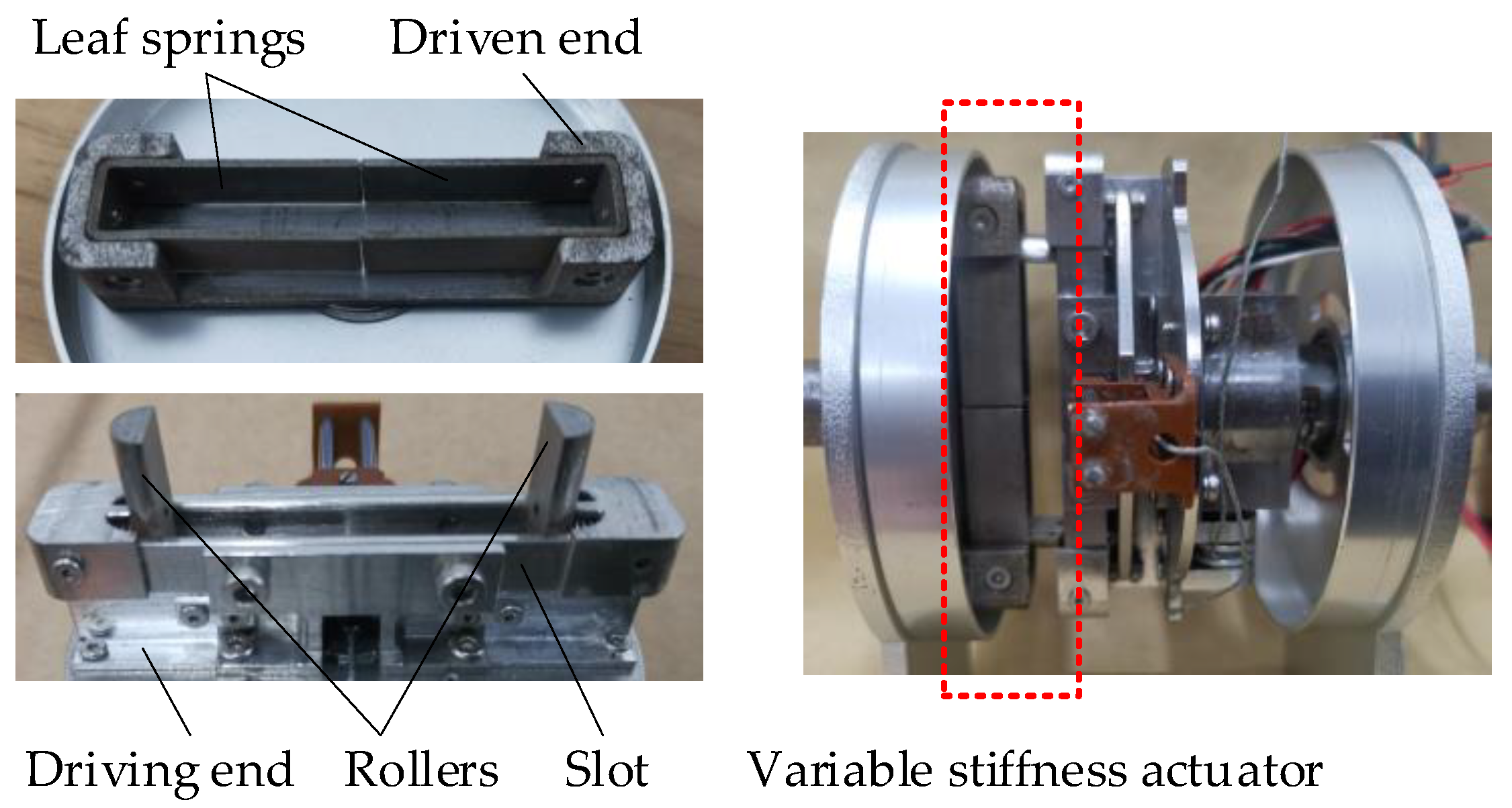
2. Composition and Configuration Design

The variable stiffness actuator is mainly composed of leaf springs, rollers and a rotating center. The leaf springs are placed on the base in a cantilever, and the rollers rotate around the rotating center. When the rollers are subjected to the moment around the rotating center, they squeeze the leaf springs and transmit the moment to the leaf springs, and then to the base. If the distance between the rollers and the rotating center changes, the length of the effective moment arm between the rollers’ pressing force and the fixed end of the leaf springs changes accordingly. Then, the deflection at the place where the leaf springs are stressed also changes, which results in change of transmission stiffness. In this way, a rigid motion is transformed from the driving end of the joint where the rollers are located, to a flexible motion through the variable stiffness actuator, and is transmitted to the driven end of the joint where the leaf springs are located. The performance of the variable stiffness actuator is related to its structural configuration, which is depends on the number, arrangement and relative positions of the components. However, existing research [39,40] mostly considers a single configuration (two rollers clamping a leaf spring), but the layout has not been analyzed in detail. Therefore, this section presents a configuration design method for the actuator, and considers the advantages and disadvantages, holistically, of several design issues, including the relative position of leaf spring and roller, the position of rotating center and the spatial arrangement of actuator.

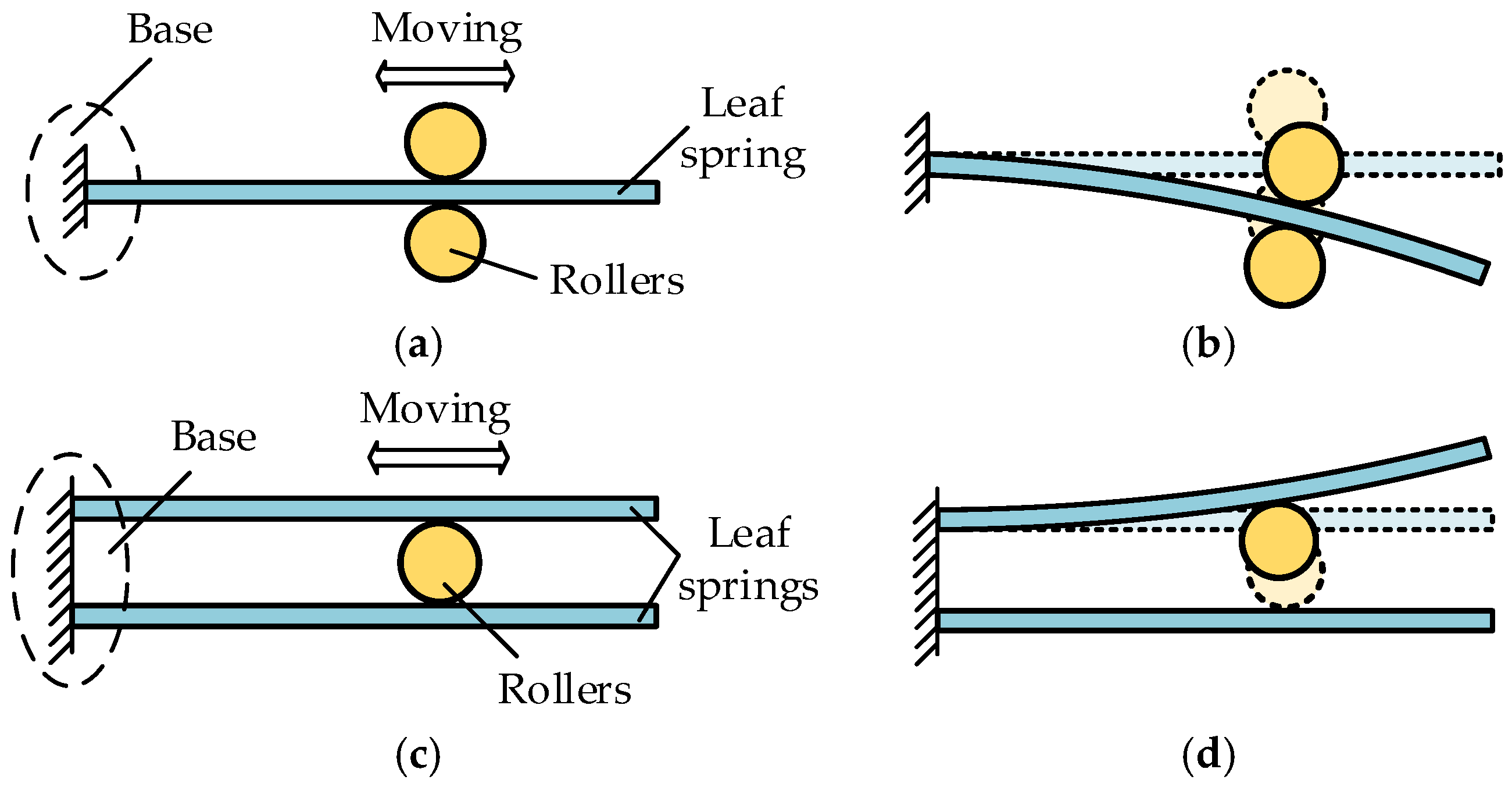
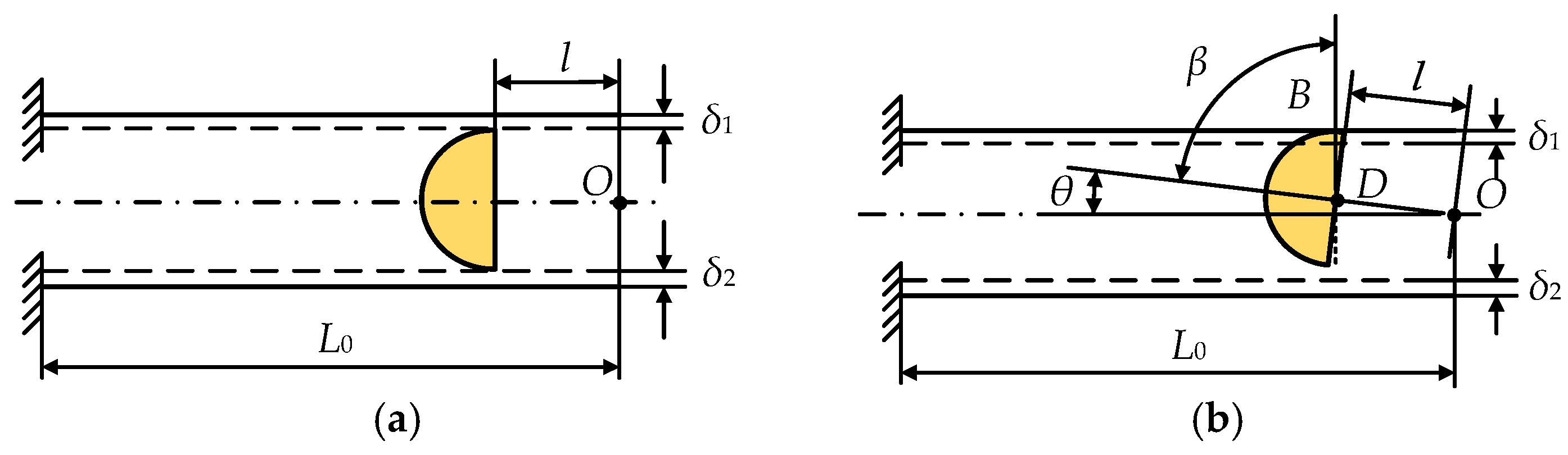
2.1. Arrangement of Leaf Springs and Rollers

According to the number and contact of leaf springs and rollers, their positions can be designed as single leaf spring and double rollers and double leaf springs and single roller, as shown in Figure 1. In this paper, the initial state of the actuator is defined as the state in which the leaf springs and the rollers do not interact with each other, and the transmission state is defined as the state where they squeeze each other. With single leaf spring and double rollers, the rollers always exert a pressing force on the leaf spring except in the initial state, so that only one leaf spring always stressed and likely to creep. However, in the double leaf springs and single roller mode, the leaf springs deform alternately in the process of reciprocating force on the actuator, thus prolonging the service life of components.

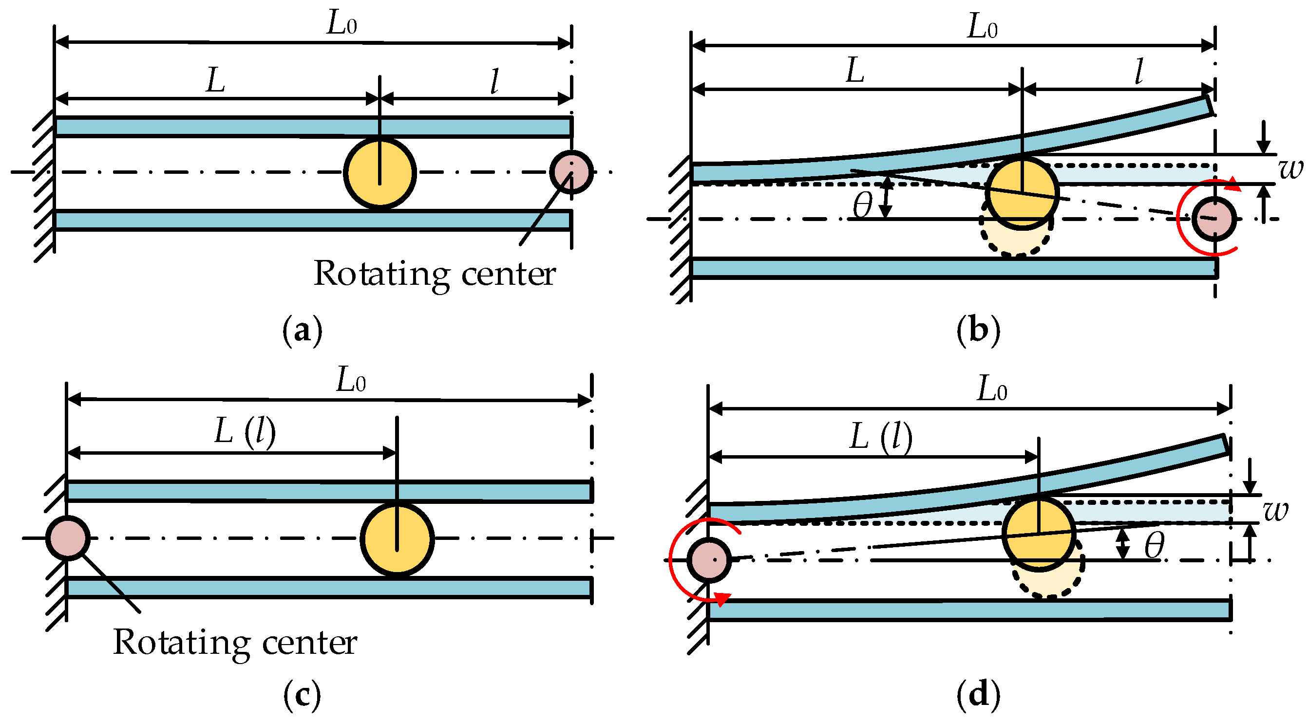
2.2. Position of the Rotating Center

Considering the relative position between the rotating center and the leaf springs. The rotating center can be placed at the free end or the fixed end of the leaf springs, as shown in Figure 2. L₀ is the initial length of the leaf spring, l is the distance between the roller and the rotating center, L is the distance between the rotating center and the fixed end, w is the deflection of the free end, and θ is the flexible rotating angle at which the roller rotates around the rotating center. The variable stiffness actuator is at the initial state when θ = 0. In Figure 2, 0 ≤ l ≤ L₀ and 0 ≤ L ≤L₀.

If the radius of the roller is very small, when the rotating center is located at the free end and the fixed end of the leaf spring, the deflections at the free end are, respectively,

$$w_1=\left(L_0-L\right)\sin \theta$$

(1)

$$w_2=L\sin \theta$$

(2)

and when the leaf spring is subjected to a force in the vertical direction at the free end, the approximate deflection is

$$w=\frac{F_y{L}^3}{3EI}$$

(3)

where F_y is the extrusion force of the leaf spring, and L equals the length of the effective arm of F_y. In Figure 2, the extrusion force between the leaf spring and the roller in these two cases are

$${\mathit{F}}_{\mathit{y}1}=\frac{3\mathit{EI}\left({\mathit{L}}_0-\mathit{L}\right)\sin \theta }{{\mathit{L}}^3}$$

(4)

$${\mathit{F}}_{\mathit{y}2}=\frac{3\mathit{EI}\sin \theta }{{\mathit{L}}^2}$$

(5)

when θ ≠ 0

$$\{\begin{array}{l}0\le F_{y1}<\infty , F_{y1} = \infty \mathrm{if} L = 0, F_{y1} = 0 \mathrm{if} L = L_0\\ F_{y2\min }\le F_{y2}<\infty , F_{y2} = \infty \mathrm{if} L = 0, F_{y2} = F_{y2\min } = \frac{3EI\sin \theta }{L_0{}^2} \mathrm{if} L = L_0\end{array}$$

(6)

Therefore, when the rotating center is located at the free end of the leaf spring, the range of extrusion force between the leaf spring and the roller is larger, and is the range of transmitted torque.

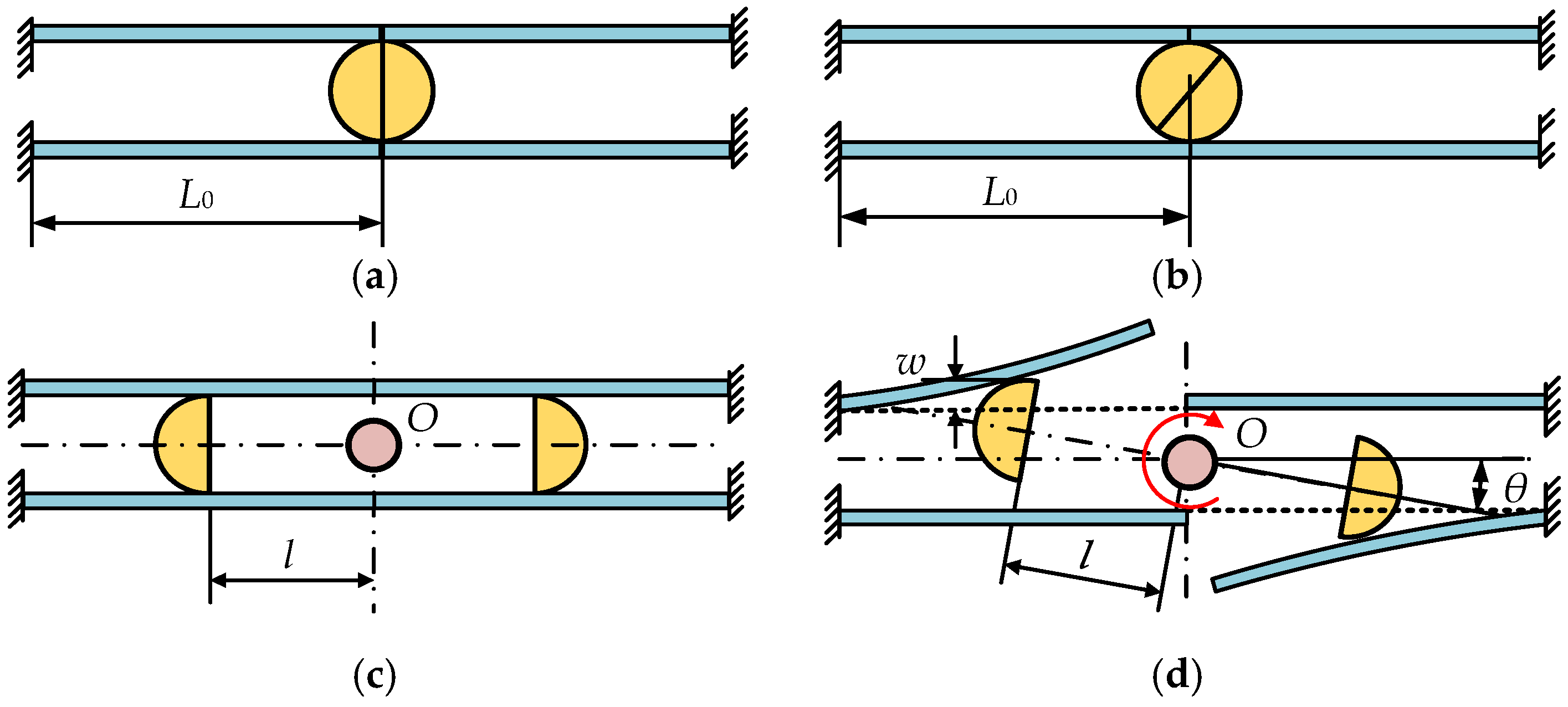
2.3. Spatial Arrangement of the Actuator

In order to improve the ability to transmit torque in a narrow space, two groups of double leaf springs and single roller modules are centrally symmetrically arranged on both sides of the rotating center. Both two rollers are made semi-cylindrical, between which the distance can be adjusted, and they can rotate around the rotating center together. According to this scheme, the working process of the variable stiffness actuator is shown in Figure 3.

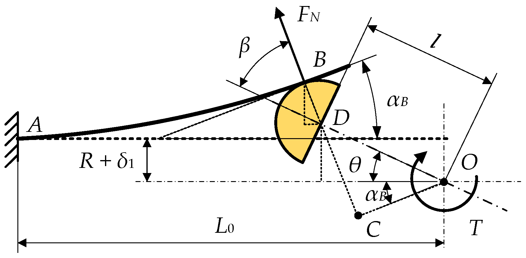
3. Mechanical Modeling and Analysis

In the existing research of variable stiffness actuators based on leaf springs, the deformation process of leaf springs is generally artificially brought to a small deflection, and an equation for small deflection of beams is used to construct the rotational stiffness model. However, such a model has shortcomings. (1) When the rotation angle is large within the large-scale deformation of the leaf spring, the small deflection equation is not applicable. (2) In existing stiffness models, the influence of parameters such as roller radius and mechanical clearance are not considered. (3) The deformation constraints are not discussed, and safety management is lacking. In this section, a general rotational stiffness model suitable for a wide deformation scale is established, and the safety criterion of flexible deformation is given, which will be the basis for stiffness control in the future.

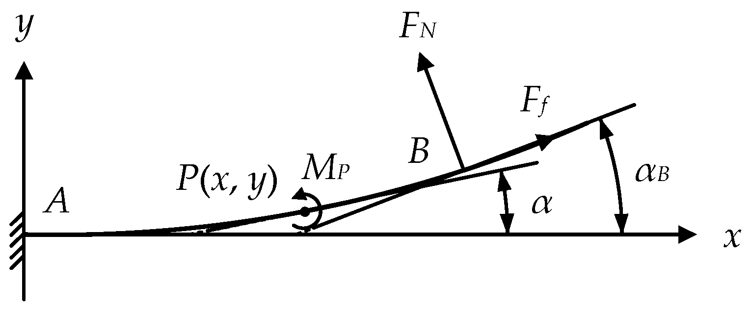
3.1. Rotational Stiffness Model

Since the variable stiffness actuator is centrosymmetric, we only analyze one symmetrical element. The mutual extrusion of leaf springs and rollers is abstracted as the problem of bending deformation of a cantilever beam under oblique load [41,42,43]. On a bending cantilever beam, a plane Cartesian coordinate system is established as shown in Figure 4, where point A is the fixed end of the leaf spring, point B is the stress point where the roller contact with the leaf spring, α is the angle between the tangent of the leaf spring at any point P on the arc $\stackrel{⌢}{AB}$ and the x-axis, α_B is the angle between the tangent of the leaf spring and the x-axis at point B, M_P is the bending moment at any point P on the arc $\stackrel{⌢}{AB}$, F_N is the support force of the leaf spring at point B by the roller, and F_f is the friction force of the leaf spring at point B.

In order to ensure repetition accuracy and smooth movement, the wear between the roller and the leaf spring should be reduced. Therefore, the contact surface between the roller and the leaf spring is extremely smooth and fully coated with lubricant. Therefore, F_f is negligible. The bending moment at point P is

$$M_P=F_N\left[\cos {\alpha }_B\left(x_B-x\right)+\sin {\alpha }_B\left(y_B-y\right)\right]$$

(7)

The exact differential equation of the deflection curve of the beam is solved as shown in Appendix A Appendix A.1 with a detailed solution process. As a result, the coordinates at point B are

$$\begin{array}{l}{x}_B=\frac{1}{\sqrt{\frac{2F_N}{EI}}}{\displaystyle {\int }_0^{{\alpha }_B}\frac{\cos \alpha \mathrm{d}\alpha }{\sqrt{\sin \left({\alpha }_B-\alpha \right)}}}\\ y_B=\frac{1}{\sqrt{\frac{2F_N}{EI}}}{\displaystyle {\int }_0^{{\alpha }_B}\frac{\sin \alpha \mathrm{d}\alpha }{\sqrt{\sin \left({\alpha }_B-\alpha \right)}}}\end{array}$$

(8)

where E is the elastic modulus of the leaf spring, and I is the cross-sectional moment of inertia. Taking one roller and the leaf spring in contact with it as a loading analysis unit, the loading state is shown in Figure 5. According to the geometric relationship in Figure 5, the coordinates of point B are

$$\begin{array}{l}{x}_B=L_0-\overline{OD}\cos \theta -\overline{BD}\cos \left(\beta +\theta \right)=L_0-l\cos \theta -R\cos \left(\beta +\theta \right)\\ y_B=OD\sin \theta +BD\sin \left(\beta +\theta \right)-R=l\sin \theta +R\sin \left(\beta +\theta \right)-R\end{array}$$

(9)

where R is the radius of the roller. In ΔCOD,

$${\alpha }_B+\theta +\beta =\frac{\pi }{2}$$

(10)

Therefore, the coordinates of point B are

$$\begin{array}{l}{x}_B=L_0-l\cos \theta -R\sin {\alpha }_B\\ y_B=l\sin \theta +R\cos {\alpha }_B-R\end{array}$$

(11)

Combining Equations (8) and (11) and cancelling out x_B and y_B, the resulting equation is converted to

$$\begin{array}{r}{L}_0-l\cos \theta -R\sin {\alpha }_B=\frac{1}{\sqrt{\frac{2F_N}{EI}}}{\displaystyle {\int }_0^{{\alpha }_B}\frac{\cos \alpha \mathrm{d}\alpha }{\sqrt{\sin \left({\alpha }_B-\alpha \right)}}}\\ l\sin \theta +R\cos {\alpha }_B-R=\frac{1}{\sqrt{\frac{2F_N}{EI}}}{\displaystyle {\int }_0^{{\alpha }_B}\frac{\sin \alpha \mathrm{d}\alpha }{\sqrt{\sin \left({\alpha }_B-\alpha \right)}}}\end{array}$$

(12)

In addition to structural parameters, there are three unknown variables including F_N, θ, and α_B in two equations of Formula (12). This can be transformed into the mapping relationship of θ concerning F_N and α_B. We set

$$\begin{array}{l}{F}_1\left({\alpha }_B\right)={\displaystyle {\int }_0^{{\alpha }_B}\frac{\cos \alpha \mathrm{d}\alpha }{\sqrt{\sin \left({\alpha }_B-\alpha \right)}}}\\ F_2\left({\alpha }_B\right)={\displaystyle {\int }_0^{{\alpha }_B}\frac{\sin \alpha \mathrm{d}\alpha }{\sqrt{\sin \left({\alpha }_B-\alpha \right)}}}\end{array}$$

(13)

F₁(α_B) and F₂(α_B) can be solved by numerical integration as in Appendix A Appendix A.2. The ratio of two equations of Formula (12) is

$$\frac{L_0-l\cos \theta -R\sin {\alpha }_B}{l\sin \theta +R\cos {\alpha }_B-R}=\frac{F_1\left({\alpha }_B\right)}{F_2\left({\alpha }_B\right)}$$

(14)

According to Formulas (12) and (13), the normal force can be expressed as

$$F_N=\frac{EI}{2}{\left(\frac{F_1\left({\alpha }_B\right)}{L_0-l\cos \theta -R\sin {\alpha }_B}\right)}^2$$

(15)

The torque transmitted by variable stiffness actuator is

$$T=2F_N\cdot \overline{OC}=2F_N\cdot l\cos \left({\alpha }_B+\theta \right)$$

(16)

In this paper, rotational stiffness is defined as the slope of the torque T transmitted by the variable stiffness actuator changing with the generated flexible rotating angle θ, which can be expressed as

$$K=\frac{\partial T}{\partial \theta }$$

(17)

Formulas (14) to (17) are included in the rotational stiffness model. When the structural dimensions are determined, the values of L₀ and R are both fixed. Therefore, α_B, F_N, T and K depend on θ and l.

Figure 5. Loading analysis unit of the variable stiffness actuator.

Figure 5. Loading analysis unit of the variable stiffness actuator.

3.2. Safe Position Space

Safe position space of the actuator refers to the maximum value range of the relative rotating angle when all the components in the actuator are in a safe state or position. If the external disturbance causes θ to exceed this range, the controllable factors, such as the position of the roller, must be adjusted appropriately.

3.2.1. Ultimate Position of the Roller under Geometric Constraints

θ and α_B are limited by the length of the leaf spring and the position of the fixed end. The following are two extreme cases.

1.

$\sqrt{L_0{}^2+R^2}-R\le l\le L_0$

When the edge of the roller just touches the fixed point A, the roller has a certain limit position, as shown in Figure 6.

Where H is a point on AG. In ΔAHO′, O’H⊥AH, AO’ = R, O’H = R − lsinθ, and AH = L₀ − lcosθ. According to the Pythagorean theorem

$$R^2={\left(R-l\sin \theta \right)}^2+{\left(L_0-l\cos \theta \right)}^2$$

(18)

The ultimate value of the rotating angle θ is

$${\theta }_{\max I}=\arcsin \frac{L_0{}^2+L^2}{2l\sqrt{R^2+L_0{}^2}}-\arcsin \frac{L_0}{\sqrt{R^2+L_0{}^2}}$$

(19)

In this case, if the farthest point on the cylindrical surface of the roller from the rotating center is in contact with the fixed point, AO′ and OO′ are collinear. In △AOD,

$$L_0{}^2+R^2={\left(R+l\right)}^2$$

(20)

The ultimate value of the distance between the rollers is

$$l_1=\sqrt{L_0{}^2+R^2}-R$$

(21)

Since the angle of the fixed end of the cantilever beam equals 0, θ will never reach θ_maxI. Thus, the limit range of θ is

$$0\le \theta <\arcsin \frac{L_0{}^2+L^2}{2l\sqrt{R^2+L_0{}^2}}-\arcsin \frac{L_0}{\sqrt{R^2+L_0{}^2}}$$

(22)

2.

$0\le l<\sqrt{L_0{}^2+R^2}-R$

In this case, the semicircular profile of the roller is far from the fixed point A, as shown in Figure 7. If the action line of F_N passes through the rotating center O, the effective moment arm of F_N relative to O becomes 0, and the torque T = 0. Before and after point B, the torque is reversed, and the effect of flexible torque on the rotational motion of the joint changes from obstruction to driving, which is difficult to control and extremely dangerous. The position of the roller in this state is called the dangerous position.

In this state, ${\alpha }_B+\theta =\frac{\pi }{2}$. When it is substituted into Equation (14),

$$\frac{L_0-\left(l+R\right)\cos \theta }{\left(l+R\right)\sin \theta -R}=\frac{F_1\left(\frac{\pi }{2}-\theta \right)}{F_2\left(\frac{\pi }{2}-\theta \right)}$$

(23)

Therefore, the dangerous value of the rotating angle θ can be expressed as

$${\theta }_{\max II}={\theta }_{\max II}\left(l\right)$$

(24)

The value range of θ is

$$\{\begin{array}{ccc}0\le \theta <{\theta }_{\max II}& ,& 0\le l<\sqrt{L_0{}^2+R^2}-R\\ 0\le \theta <\arcsin \frac{L_0{}^2+L^2}{2l\sqrt{R^2+L_0{}^2}}-\arcsin \frac{L_0}{\sqrt{R^2+L_0{}^2}}& ,& \sqrt{L_0{}^2+R^2}-R\le l\le L_0\end{array}$$

(25)

3.2.2. Ultimate Position of the Roller Not separated from the Leaf Spring

The length of the leaf spring before and after deformation is assumed to be constant. In order to ensure that the roller is not separated from the leaf spring, that is, its cylindrical surface is always tangent to the leaf spring, so

$$\stackrel{⌢}{AB}\le L_0$$

(26)

and the arc length $\stackrel{⌢}{AB}$ can be expressed as

$$\stackrel{⌢}{AB}={\displaystyle {\int }_0^{\stackrel{⌢}{AB}}\mathrm{d}s}={\displaystyle {\int }_0^{{\alpha }_B}\frac{\mathrm{d}\alpha }{\sqrt{\frac{2}{EI}{F}_N\sin \left({\alpha }_B-\alpha \right)}}}=\sqrt{\frac{EI}{2F_N}}{\displaystyle {\int }_0^{{\alpha }_B}\frac{\mathrm{d}\alpha }{\sqrt{\sin \left({\alpha }_B-\alpha \right)}}}$$

(27)

which can be solved by the numerical method as in Appendix A Appendix A.3 for the solution process.

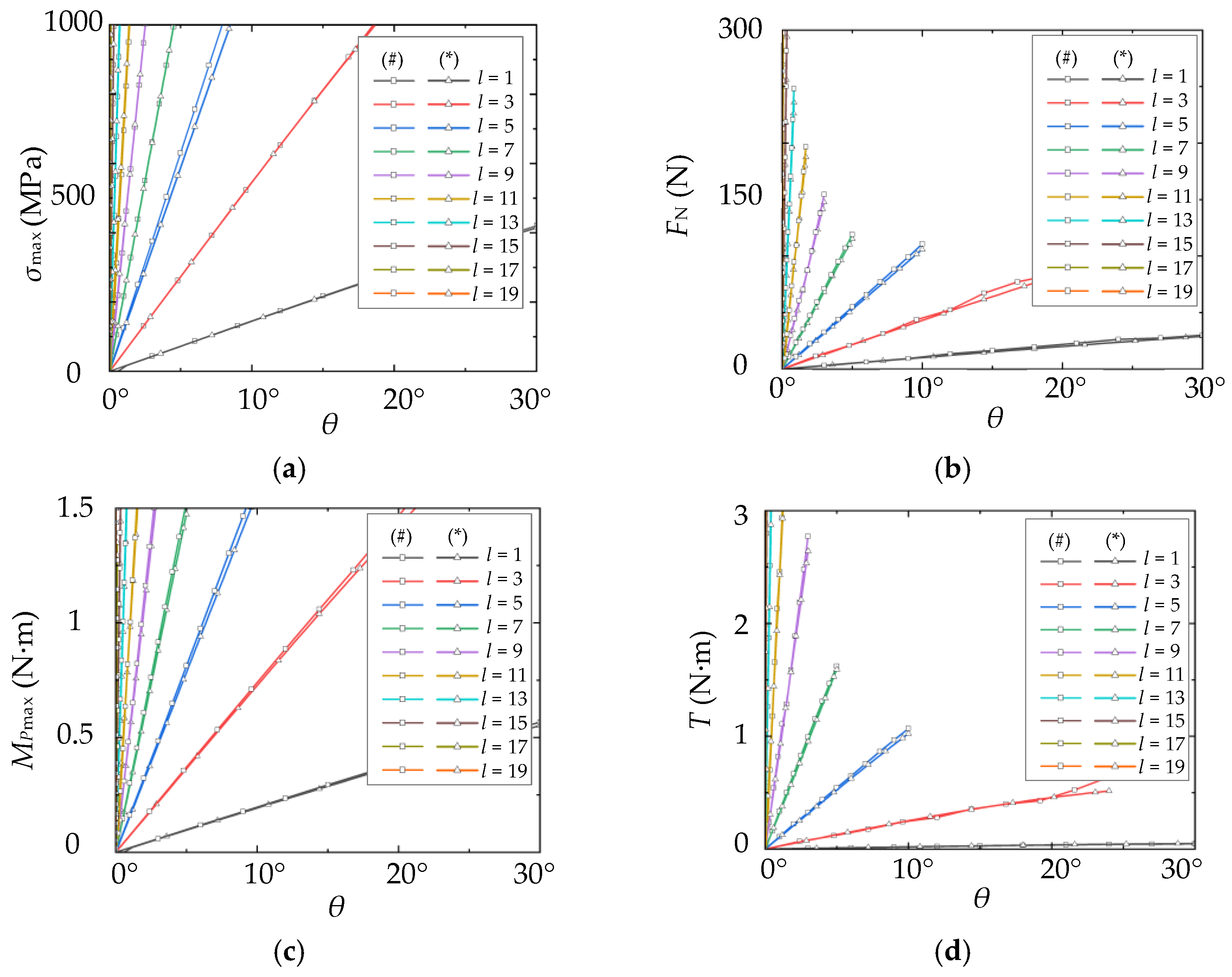
3.2.3. Ultimate Deformation of the Leaf Spring under the Constraint of Strength

The maximum normal stress in the cross-section of the leaf spring is

$${\sigma }_{\max }=\frac{M_{P\max }}{W_{\mathrm{Z}}}$$

(28)

According to Formula (7), the bending moment at the fixed point A is the greatest, which can be expressed as

$$M_{P\max }=M_A=F_N\left[x_B\cos {\alpha }_B+y_B\sin {\alpha }_B\right]$$

(29)

For a rectangle cantilever beam,

$$W_{\mathrm{Z}}=\frac{b{h}^2}{6}$$

(30)

According to the intensity condition for bending normal stress, the deformation limit of the leaf spring is

$${\sigma }_{\max }=\frac{6F_N}{b{h}^2}\left[x_B\cos {\alpha }_B+y_B\sin {\alpha }_B\right]\le {\left[\sigma \right]}_l$$

(31)

The allowable stress of the leaf spring is

$${\left[\sigma \right]}_l=\frac{{\sigma }_s}{n_l}$$

(32)

where n_l is the safety factor of the material of the leaf spring, which can be taken as n_l = 1.2.

The value range of the flexible angle θ that meets all the above three requirements is the safe position space of the actuator.

4. Stiffness-Adjusting Characteristics

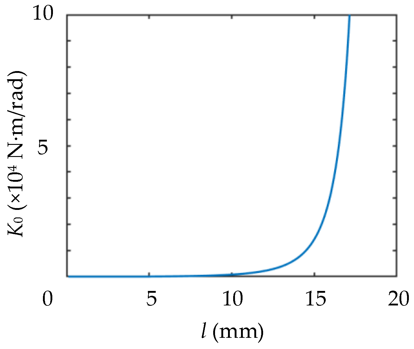
4.1. Changing Laws of Stiffness

Considering the limitation of space and design experience, it is assumed that the length of the cantilever leaf spring L₀ = 20 mm, the thickness h = 1 mm and the width b = 8 mm and the radius of the roller R = 3.5 mm. The material of the leaf spring is 60Si2CrVA, whose modulus E = 200 GPa and yield limit σ_s = 1666 MPa. According to Equation (32), the allowable stress [σ]_l = 1388 MPa. In this paper, the ultimate deformation of the leaf spring under the constraint of strength is taken as the primary condition. According to the safe position space, θ_max and corresponding α_Bmax are obtained by a numerical method, as shown in

Table 1. Values of l and corresponding θ_max and α_Bmax.

l (mm)	0	0~1	~3	~5	~7	~9	~11	~13	~15	~17	~19
θmax (°)	30	30	24	10	5	3	1.7	0.85	0.35	0.1	0.01
αBmax (°)	0	2.25	6.11	4.98	4.05	3.70	3.13	2.38	1.58	0.85	0.31

. It is verified that the values in the table are also within the scope of the ultimate position of the roller under geometric constraints and the ultimate position of the roller is not out of the leaf spring. According to Formulas (14) to (17), the relationship curves of T and K with respect to θ under different values of l are shown in Figure 8.

According to Figure 8b, in the safe position space, K increases with l but does not change obviously with θ. In a certain range, K initially increases and then decreases, mainly caused by the decreasing length of the effective arm of F_N. Therefore, the relationship between the stiffness K₀ in the initial state of the actuator and l can approximately reflect the relationship between K and l. For convenient analysis, we take a small change of the angle Δθ = 0.0001 which produces a torque ΔT. The stiffness K₀ near the initial state of the actuator can be expressed as

$$K_0=\frac{\mathsf{\Delta }T}{\mathsf{\Delta }\theta }$$

(33)

After numerical calculation, the relationship between K₀ and l is shown in Figure 9. Near the initial state, when l = 0, K₀ = 0. When l increases, K increases too, and the closer l is to L₀, the faster K increases. In theory, when l = L₀, K₀ = ∞.

4.2. Influence of Structural Parameters on the Characteristics of Adjusting Stiffness

There are many parameters and variables in the rotational stiffness model, including L₀, θ, l, R, α_B, E and I. In Formulas (14) to (17), l is a controllable variable in the working process of the actuator, θ is a passive variable, L₀ and R are structural design parameters, and α_B is an intermediate variable. When L₀ and R are determined, α_B depends on θ and L. E is a material characteristic parameter, and I is a structural design parameter. In this paper, the tendency of the stiffness K with the main variables θ and l are observed when the structural design parameters L₀, R, I and the material parameter E are changed. So that the stiffness adjustment characteristics of the actuator are analyzed, which provides an important reference for the subsequent structural design and product serialization.

4.2.1. The Thickness h and Width b of the Cantilever Leaf Spring

The leaf spring is a cuboid structure, whose width is b and thickness is h. The moment of inertia is given by

$$I=\frac{b{h}^3}{12}$$

(34)

Therefore, the thickness h and width b of the cantilever leaf spring define the cross-sectional moment of inertia I, thus affecting the characteristics of adjusting stiffness. According to Formulas (34) and (15)

$$F_N\propto b{h}^3$$

(35)

$$T\propto F_N, K\propto T$$

(36)

Therefore $K\propto b{h}^3$, namely the thickness h and width b of cantilever leaf spring, only affect the value of stiffness, but not the changing trend. The larger h and b, the greater the stiffness K under the corresponding θ and l. Compared with b, h has a more obvious influence on the changing trend of stiffness.

4.2.2. The Modulus E of the Cantilever Leaf Spring

E affects the stiffness adjustment characteristics by changing the material stiffness EI of the leaf spring. According to Formula (15),

$$F_N\propto E$$

(37)

Therefore $K\propto E$ according to Formula (36).

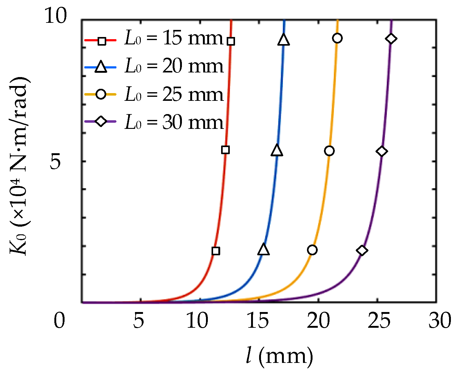
4.2.3. The Length of the Cantilever Leaf Spring L₀

Because changing θ has little influence on K within the safe position space, we only studied the influence of L₀ on K₀. If h = 1 mm, b = 8 mm and R = 3.5 mm, the stiffness curves near the initial state when L₀ = 15, 20, 25 and 30 mm are shown in Figure 10. When l is much smaller than L₀, K is kept at a low value. When l is equivalent to L₀, K₀ increases with l and the speed increases. Therefore, a smaller L₀ is beneficial to ensure the compactness of the structure, while increasing L₀ is beneficial for widening the low stiffness area, thus improving the accuracy of the adjusting stiffness in this area.

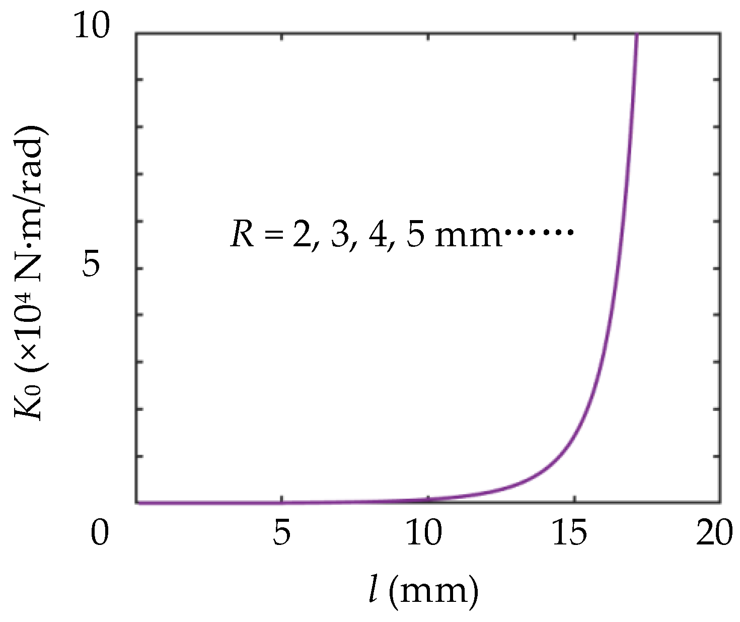
4.2.4. Roller Radius R

Similar to the length of the cantilever leaf spring, we only studied the influence of roller radius R on K₀. In this section, h = 1 mm, b = 8 mm and L₀ = 20 mm. It can be seen from Figure 11 that curves of changing K₀ coincide with each other under different values of R. Thus, the value of R has no effect on K₀. Therefore, the value of R mainly affects the safe position space of the variable stiffness actuator but has little effect on the whole process of adjusting stiffness.

4.3. Influence of Clearance on the Characteristics of Adjusting the Stiffness

In the installation process, there may be a clearance between the roller and the leaf springs. The widths of two installation clearance areas on both sides of the roller are expressed as δ₁ and δ₂, as shown in Figure 12. For the convenience of analysis, we take clearance δ1 as an example. When the roller is in the position shown in Figure 12b, the roller is just in contact with the leaf spring. In this case,

$${\beta }_1+{\theta }_1=\frac{\pi }{2}$$

(38)

$${\delta }_1=l\sin {\theta }_1$$

(39)

and the critical angle is

$${\theta }_1=\arcsin \frac{{\delta }_1}{l}$$

(40)

The working state of the actuator is analyzed in the following two situations.

1.

$0\le \theta <{\theta }_1$;

In this case, if the roller is not in contact with the leaf spring, F_N = 0, T = 0 and K = 0. Therefore, the clearance leads to a zero-stiffness region. If the zero-stiffness region is small, it acts as a buffer and a safety feature when the actuator is subjected to an instantaneous impact load. However, if the zero-stiffness region is too large, it will have a great adverse impact on the system. Thus, the machining accuracy should be improved as much as possible to reduce the zero-stiffness region.

2.

$\theta \ge {\theta }_1$;

As shown in Figure 13, the roller crosses the critical position and squeezes the cantilever leaf spring to deform. Then, Formula (11) is converted to

$$\begin{array}{l}{x}_B=L_0-l\cos \theta -R\sin {\alpha }_B\\ y_B=l\sin \theta +R\cos {\alpha }_B-\left(R+{\delta }_1\right)\end{array}$$

(41)

Formula (14) is converted into

$$\frac{L_0-l\cos \theta -R\sin {\alpha }_B}{l\sin \theta +R\cos {\alpha }_B-\left(R+{\delta }_1\right)}=\frac{F_1\left({\alpha }_B\right)}{F_2\left({\alpha }_B\right)}$$

(42)

According to the actually measured curve of stiffness, the value of the critical rotation angle θ₁ can be obtained, and then the value of δ₁ can be calculated by Formula (39). By substituting δ₁ into Equation (42), the stiffness model can be revised.

Figure 13. Force diagram of the variable stiffness actuator with clearance (transmission state).

Figure 13. Force diagram of the variable stiffness actuator with clearance (transmission state).

5. Static Simulation and Test

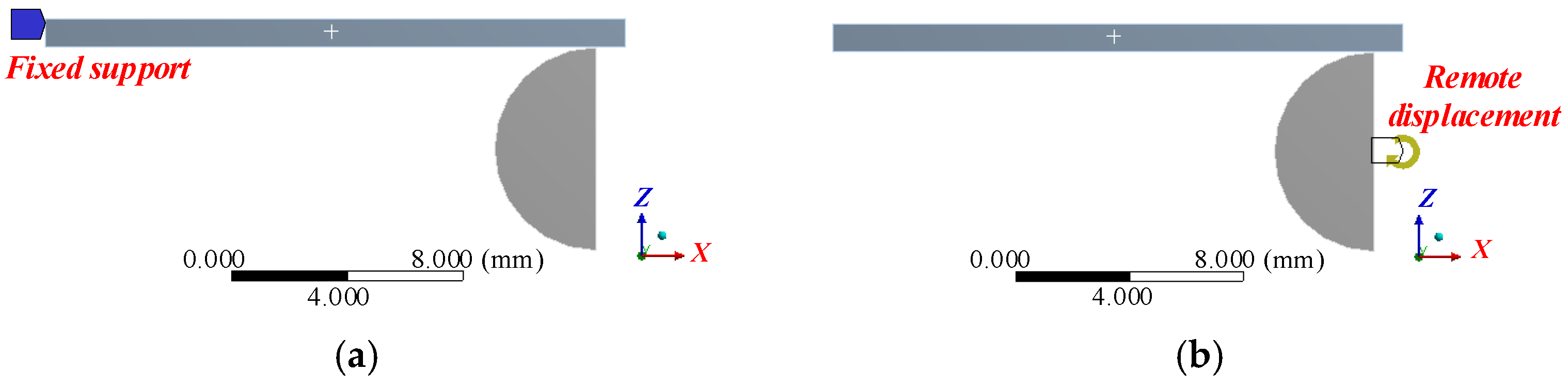
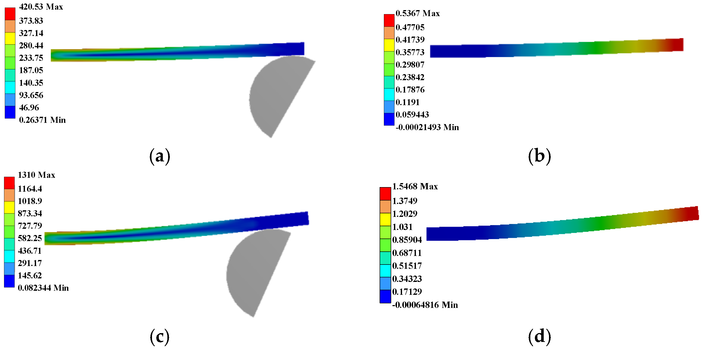
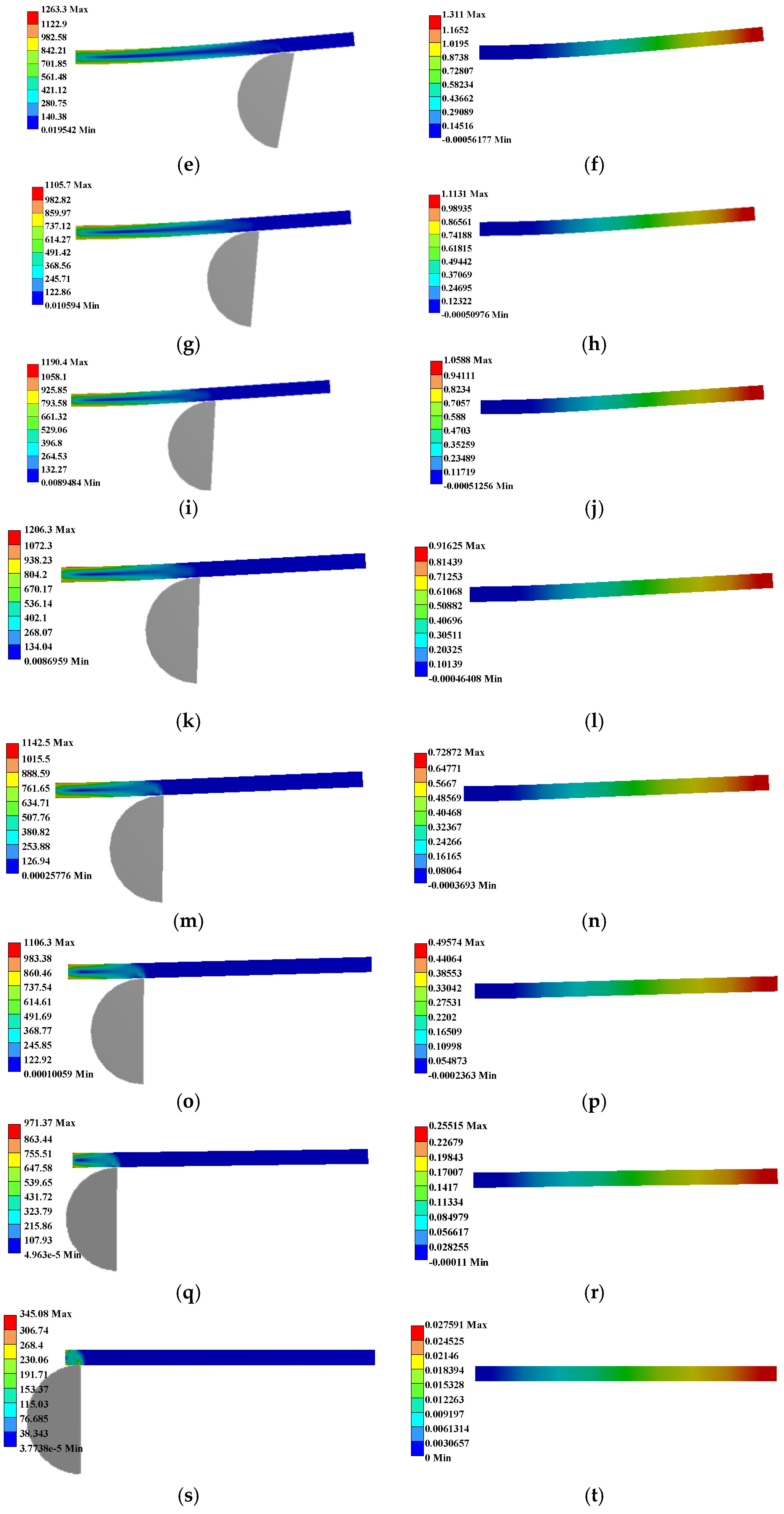
5.1. Finite Element Simulation

To verify the rotational stiffness model, static analysis was carried out using the finite element analysis method. Finite element analysis can monitor the deformation, stress, force and moment in the process of loading, some of which are intermediate variables of the rotational stiffness model and difficult to measure directly by experiments. The simulation settings are shown in Figure 14. Fixed support is applied at one end of the leaf spring, and a remote rotating angle relative to point O is applied on the roller. The deformation and stress of the leaf spring are simulated when θ reaches the ultimate value under different values of l, in which l and θ are taken according to Table 1.

When the rotating angle reaches the maximum value, the maximum normal stress and the maximum displacement in the y direction of the leaf spring are obtained, as shown in

Table 2. Maximum stress σ_max and deformation d_ymax of the leaf spring.

l (mm)	1	3	5	7	9	11	13	15	17	19
σmax (Mpa)	421	1310	1263	1106	1190	1206	1142	1106	971	345
dymax (mm)	0.537	1.547	1.311	1.113	1.057	0.916	0.787	0.496	0.255	0.028

. The deformation and stress state of the leaf spring are shown in Figure 15. In the process of deformation, the maximum stress of the leaf spring is at a fixed point and never exceeds [σ]_l. The maximum stress σ_max, the reaction force F_N of the contact point, the moment M_Pmax (M_A) of the fixed end and the moment T of the rotating center directly obtained by simulation are compared with data calculated by the model, as shown in Figure 16. Results show the rotational stiffness model is highly accurate.

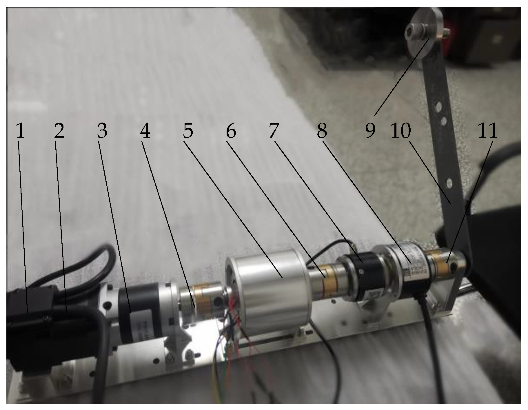
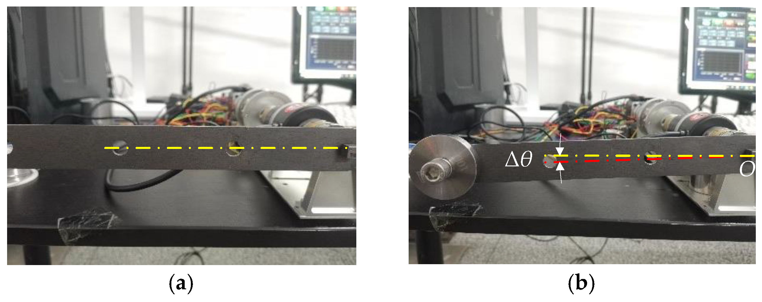
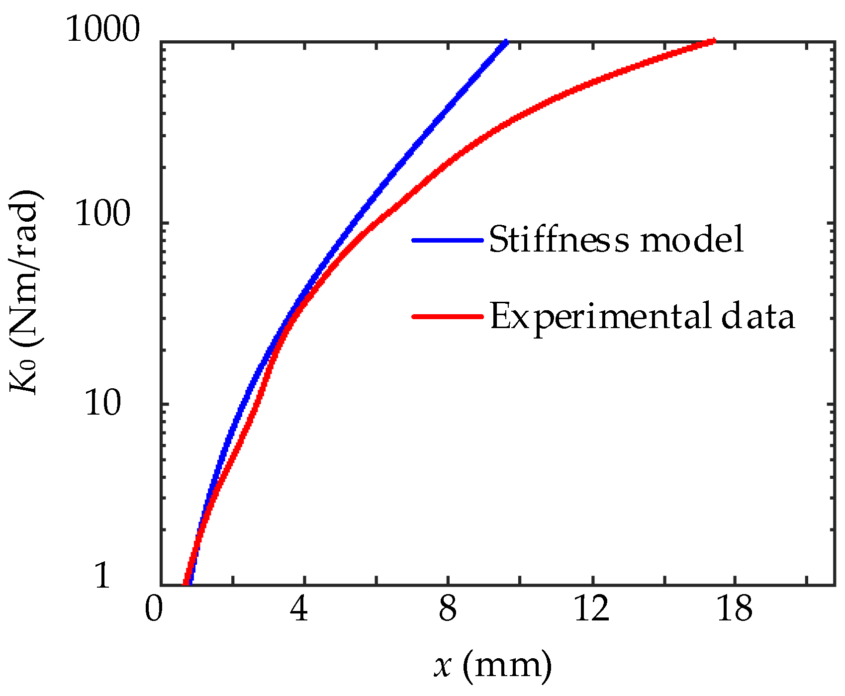
5.2. Identification Test of Static Stiffness

In order to verify that the variable stiffness actuator can effectively adjust stiffness in the joint, a prototype of the variable stiffness joint and a test platform was developed. The prototype of the joint is shown in Figure 17. The variable stiffness actuator is installed inside the joint. Two leaf springs are symmetrically installed at the driven end of the joint, and two rollers are located at the driving end of the joint which can slide in the slot. The driving end of the joint transmits the force and motion to the driven end through the variable stiffness actuator. The test platform is shown in Figure 18. In the test platform, one end of the joint is connected with a position motor and a reducer so that a dynamic test can be carried out. The other end of the joint is connected with a connecting rod and a counterweight representing the load of the joint. An angular displacement sensor is installed between the joint and the connecting rod and is used to measure the flexible rotating angle θ. In addition, a torque sensor is installed between the joint and the displacement sensor to measure the torque T.

A static stiffness identification test was conducted to observe the stiffness adjustment function of the actuator by observing the change of the relative rotating angle between the driving and driven ends under the static torque. First, the position motor was enabled for braking, and the rollers in the actuator reached different predetermined positions. Then, the connecting rod was loaded at different positions by different masses of counterweights. Finally, we measured the data and calculated the actual value of stiffness using Formula (33). Inside the joint, the position of the roller is controlled by the rope pulling mechanism driven by a stiffness-adjusting motor. There is a unique mapping relationship between the displacement x of the pulling rope and the distance between the rollers and the rotating center l, which is

$$x=x(l)$$

(43)

For convenience, x was used instead of l in the test. When measuring x, the size and position of the counterweight were adjusted at the same time. Then the value of torque measured by the torque sensor and the rotating angle measured by the angular sensor were recorded. The joint was loaded both in forward and reverse, and the angle was strictly limited according to the safe position space of the actuator, preventing the structural members such as the leaf springs and the rollers from being damaged. The relationship between the loading torque, the mass of the counterweight and the length of the force arm is shown in

Table 3. The value of torque loading by counterweight (N·m).

	Length of Force Arm (mm)	50	100	150
Mass of the Counterweight (kg)
0.1		0.08	0.15	0.23
0.2		0.15	0.29	0.44
0.3		0.24	0.45	0.68
0.5		0.37	0.74	1.13
1.0		0.75	1.48	2.23
2.0		1.52	2.96	4.46
3.0		2.32	4.54	6.76

.

During the test, it was necessary to avoid the influence of clearance between the leaf springs and the rollers and in the couplings. Therefore, we adjusted the connecting rod to the horizontal state for preloading to eliminate the clearance and recorded the torque T₀ at this time. Then, we reset the angular encoder and installed the counterweight. If the torque sensor is T, the actual loading torque is

$$\mathsf{\Delta }T=T-T_0$$

(44)

The test platform before and after static loading is shown in Figure 19a,b. The yellow line and the red line are the symmetry lines of the connecting rod before and after loading, Δθ is the angle between them, and O is the rotating center. When the joint was subjected to a torque of 10 N·m, the variable stiffness actuator was still not damaged. The tested curve of ΔT−Δθ is shown in Figure 20. It can be seen that the relationship curve between ΔT and Δθ is approximately a straight line, that is, the stiffness value was basically constant during the process of small deformation. The curve becomes bent at some positions, caused by insufficient measurement accuracy of the angular encoder and the instability of the pulse collector near the zero position.

According to Formula (33), the curve of K₀−x was drawn and smoothed and is compared with the theoretical curve shown in Figure 21. It can be seen that the stiffness increases with x, and the increasing speed becomes faster and faster, which is consistent with the theoretical results. The maximum stiffness exceeds 1000 Nm/rad. In the range of a small driving displacement when x = 0~5 mm, the stiffness is in good agreement with the theoretical value. When x increases, the difference between the result of stiffness adjustment and the theoretical value becomes larger. The main reasons for this phenomenon are:

(1)

The long transmission path of the test bed leads to greater flexibility of the system, which makes the measured value of stiffness smaller than the actual value.

(2)

The resolution of the encoder is not enough to identify the minimal angular displacement, so that the encoder cannot truly reflect the angular deformation when the stiffness is high.

Therefore, in the working process, it is necessary to reduce the mechanical clearance as much as possible, increase the rigidity of the transmission shaft, and adopt higher-precision sensors to adjust the stiffness with high-precision.

Figure 21. Fitting curve of experimental values and model values of K₀.

Figure 21. Fitting curve of experimental values and model values of K₀.

6. Conclusions

In this research, a variable stiffness actuator based on a leaf spring was investigated by designing, modelling, simulation and experiments. The research reveals the following. (1) With our overall configuration design method, a configuration of double leaf springs and single roller with a symmetrical arrangement and rotating center at the free end of leaf springs has the advantages of large bearing capacity, safety and reliability. (2) A rotational stiffness model with universality and high-accuracy was constructed, which is suitable when the actuator deforms within the safe position space. To allow the actuator to operate safely, the leaf springs should always block the movement of the rollers so that the rollers do not come out from the free end of the leaf springs, and the leaf springs avoid plastic deformation. (3) Stiffness increases with the distance between the rollers and the rotating center, and the growth rate accelerates. The thickness, width and modulus of the springs affect the magnitude of stiffness. The radius of the rollers affects the safe position space. The installation clearance leads to a zero-stiffness area, and a small clearance is beneficial to alleviate the impact. (4) The rotational stiffness model was verified by a finite element method. Static tests show that the actuator can effectively adjust the stiffness of the joint, and the range of stiffness was 0~1000Nm/rad. In the low stiffness region, the actual stiffness had a high coincidence with the theoretical value. If the processing and assembly of parts are improved and high-precision sensors are used, the stiffness could be controlled more accurately.

References

1. Siddaramaiah, V.H.; Calderon, D.E.; Cooper, J.E.; Wilson, T. Preliminary Studies in the Use of Folding Wing-Tips for Loads Alleviation. In Proceedings of the Royal Aeronautical Society Aerodynamics Conference, Bristol, UK, 22–24 July 2014; pp. 724–737. [Google Scholar]
2. Wen, M.; Yu, M.; Fu, J.; Wu, Z.; Cui, J.; Tan, J.; Wen, X. Multi-Functional Hinge Equipped with A Magneto-Rheological Rotary Damper for Solar Array Deployment System. In Proceedings of the SPIE-The International Society for Optical Engineering, Changsha/Zhangjiajie, China, 6 March 2015; p. 944648. [Google Scholar]
3. Guo, J.; Tian, G. Mechanical Design and Analysis of the Novel 6-DOF Variable Stiffness Robot Arm Based on Antagonistic Driven Joints. J. Intell. Robot. Syst. 2015, 82, 207–235. [Google Scholar] [CrossRef]
4. Tang, D.; Dowell, E.H. Theoretical and Experimental Aeroelastic Study for Folding Wing Structures. J. Aircr. 2008, 45, 1136–1147. [Google Scholar] [CrossRef]
5. He, J.; Zhang, Y.; Shangguan, Z.; Yang, L. A Review of Bionic Design in Satellite Solar Wing Structures. J. Phys. Conf. Ser. 2020, 1549, 042099. [Google Scholar] [CrossRef]
6. Choi, J.; Park, S.; Lee, W.; Kang, S. Design of a Robot Joint with Variable Stiffness. In Proceedings of the 2008 IEEE International Conference on Robotics and Automation, Pasadena, CA, USA, 19–23 May 2008; pp. 1760–1765. [Google Scholar]
7. Hyun, M.W.; Yoo, J.; Hwang, S.T.; Choi, J.H.; Kang, S.; Kim, S.-J. Optimal Design of a Variable Stiffness Joint Using Permanent Magnets. IEEE Trans. Magn. 2007, 43, 2710–2712. [Google Scholar] [CrossRef]
8. Boehler, Q.; Vedrines, M.; Abdelaziz, S.; Poignet, P.; Renaud, P. Design and Evaluation of a Novel Variable Stiffness Spherical Joint with Application to MR-Compatible Robot Design. In Proceedings of the 2016 IEEE International Conference on Robotics and Automation (ICRA), Stockholm, Sweden, 16–21 May 2016; pp. 661–667. [Google Scholar] [CrossRef] [Green Version]
9. Sun, Y.; Tang, P.; Dong, D.; Zheng, J.; Chen, X.; Bai, L. Modeling and Experimental Evaluation of a Pneumatic Variable Stiffness Actuator. IEEE/ASME Trans. Mechatron. 2021, 1–12. [Google Scholar] [CrossRef]
10. Kajikawa, S.; Ito, T.; Hase, H. Stiffness Control of Variable Stiffness Joint Using Electromyography Signals. In Proceedings of the 2013 IEEE International Conference on Robotics and Automation, Karlsruhe, Germany, 6–10 May 2013; pp. 4928–4933. [Google Scholar] [CrossRef]
11. Kajikawa, S.; Yonemoto, Y. Joint Mechanism with a Multi-Directional Stiffness Adjuster. In Proceedings of the 2010 IEEE/RSJ International Conference on Intelligent Robots and Systems, Taipei, Taiwan, 18–22 October 2010; pp. 4194–4200. [Google Scholar]
12. Heepe, L.; Gorb, S.N. Biologically Inspired Mushroom-Shaped Adhesive Microstructures. Annu. Rev. Mater. Sci. 2014, 44, 173–203. [Google Scholar] [CrossRef]
13. Huber, G.; Gorb, S.N.; Spolenak, R.; Arzt, E. Resolving the Nanoscale Adhesion of Individual Gecko Spatulae by Atomic Force Microscopy. Biol. Lett. 2005, 1, 2–4. [Google Scholar] [CrossRef] [Green Version]
14. Hauser, S.; Robertson, M.; Ijspeert, A.; Paik, J. JammJoint: A Variable Stiffness Device Based on Granular Jamming for Wearable Joint Support. IEEE Robot. Autom. Lett. 2017, 2, 849–855. [Google Scholar] [CrossRef]
15. Li, Y.; Chen, Y.; Yang, Y.; Wei, Y. Passive Particle Jamming and Its Stiffening of Soft Robotic Grippers. IEEE Trans. Robot. 2017, 33, 446–455. [Google Scholar] [CrossRef]
16. Li, J.; Zhong, G.; Yin, H.; He, M.; Tan, Y.; Li, Z. Position control of a robot finger with variable stiffness actuated by shape memory alloy. In Proceedings of the 2017 IEEE International Conference on Robotics and Automation (ICRA), Singapore, 29 May 2017–3 June 2017; pp. 4941–4946. [Google Scholar] [CrossRef]
17. Chautems, C.; Tonazzini, A.; Floreano, D.; Nelson, B.J. A Variable Stiffness Catheter Controlled with an External Magnetic Field. In Proceedings of the 2017 IEEE/RSJ International Conference on Intelligent Robots and Systems (IROS), Vancouver, BC, Canada, 24–28 September 2017; pp. 181–186. [Google Scholar] [CrossRef]
18. Zhao, J.; Niu, J.; McCoul, D.; Leng, J.; Pei, Q. A Rotary Joint for a Flapping Wing Actuated by Dielectric Elastomers: Design and Experiment. Meccanica 2015, 50, 2815–2824. [Google Scholar] [CrossRef]
19. Wen, W.; Huang, X.; Sheng, P. Electrorheological Fluids: Structures and Mechanisms. Soft Matter 2007, 4, 200–210. [Google Scholar] [CrossRef] [PubMed]
20. Bahl, S.; Nagar, H.; Singh, I.; Sehgal, S. Smart Material Types, Properties and Applications: A Review. Mater. Today Proc. 2020, 28, 1302–1306. [Google Scholar] [CrossRef]
21. Nikitczuk, J.; Weinberg, B.; Canavan, P.K.; Mavroidis, C. Active Knee Rehabilitation Orthotic Device with Variable Damping Characteristics Implemented via an Electrorheological Fluid. IEEE/ASME Trans. Mechatron. 2009, 15, 952–960. [Google Scholar] [CrossRef]
22. Davidson, J.R.; Krebs, H.I. An Electrorheological Fluid Actuator for Rehabilitation Robotics. IEEE/ASME Trans. Mechatron. 2018, 23, 2156–2167. [Google Scholar] [CrossRef]
23. Wei, W.; Cai, S.; Bian, G.; Bao, G.; Yu, J.; Yang, D.; Zhang, L. Control of Compliant Joint Based on Magneto-rheological Fluid Coupling Transmission. In Proceedings of the 2019 IEEE 4th International Conference on Advanced Robotics and Mechatronics (ICARM), Toyonaka, Japan, 3–5 July 2019; pp. 1–6. [Google Scholar] [CrossRef]
24. Mao, Z.; Iizuka, T.; Maeda, S. Bidirectional Electrohydrodynamic Pump with High Symmetrical Performance and Its Application to a Tube Actuator. Sens. Actuators A Phys. 2021, 332, 113168. [Google Scholar] [CrossRef]
25. Mao, Z.; Asai, Y.; Yamanoi, A.; Seki, Y.; Wiranata, A.; Minaminosono, A. Fluidic Rolling Robot Using Voltage-Driven Oscillating Liquid. Smart Mater. Struct. 2022, 31, 1–10. [Google Scholar] [CrossRef]
26. Awad, M.I.; Gan, D.; Cempini, M.; Cortese, M.; Vitiello, N.; Dias, J.; Dario, P.; Seneviratne, L. Modeling, design & character-ization of a novel passive variable stiffness joint (pVSJ). In Proceedings of the 2016 IEEE/RSJ International Conference on Intelligent Robots and Systems (IROS), Daejeon, Korea, 9–14 October 2016; pp. 323–329. [Google Scholar]
27. Jafari, A.; Tsagarakis, N.G.; Caldwell, D.G. AwAS-II: A New Actuator with Adjustable Stiffness Based on the Novel Principle of Adaptable Pivot Point and Variable Lever Ratio. In Proceedings of the 2011 IEEE International Conference on Robotics and Automation, Shanghai, China, 9–13 May 2011; pp. 4638–4643. [Google Scholar]
28. Yin, P.; Li, M.; Guo, W.; Wang, P.; Sun, L. Design of a Unidirectional Joint with Adjustable Stiffness for Energy Efficient Hopping Leg. In Proceedings of the 2013 IEEE International Conference on Robotics and Biomimetics (ROBIO), Shenzhen, China, 12–14 December 2013; pp. 2587–2592. [Google Scholar] [CrossRef]
29. Jafari, A.; Tsagarakis, N.G.; Sardellitti, I.; Caldwell, D.G. A New Actuator with Adjustable Stiffness Based on a Variable Ratio Lever Mechanism. IEEE/ASME Trans. Mechatronics 2012, 19, 55–63. [Google Scholar] [CrossRef]
30. Yang, D.; Jin, H.; Liu, Z.; Fan, J.; Zhu, Y.; Zhang, H.; Dong, H. Design and Modeling of a Torsion Spring-Based Actuator (TSA) With Valid Straight-Arm Length Adjustable for Stiffness Regulation. In Proceedings of the 2016 IEEE International Conference on Mechatronics and Automation, Harbin, China, 7–10 August 2016; pp. 2381–2386. [Google Scholar] [CrossRef]
31. Liu, Y.; Liu, X.; Yuan, Z.; Liu, J. Design and Analysis of Spring Parallel Variable Stiffness Actuator Based on Antagonistic Principle. Mech. Mach. Theory 2019, 140, 44–58. [Google Scholar] [CrossRef]
32. Choi, J.; Hong, S.; Lee, W.; Kang, S. A Variable Stiffness Joint Using Leaf Springs for Robot Manipulators. In Proceedings of the 2009 IEEE International Conference on Robotics and Automation, Kobe, Japan, 12–17 May 2009; pp. 4363–4368. [Google Scholar] [CrossRef]
33. Morita, T.; Sugano, S. Development of an anthropomorphic force-controlled manipulator WAM-10. In Proceedings of the 1997 8th International Conference on Advanced Robotics. Proceedings. ICAR’97, Monterey, CA, USA, 7–9 July 1997. [Google Scholar] [CrossRef]
34. Barrett, E.; Fumagalli, M.; Carloni, R. Elastic Energy Storage in Leaf Springs for a Lever-Arm Based Variable Stiffness Actuator. In Proceedings of the 2016 IEEE/RSJ International Conference on Intelligent Robots and Systems (IROS), Daejeon, Korea, 9–14 October 2016; pp. 537–542. [Google Scholar] [CrossRef]
35. Wu, J.; Wang, Z.; Chen, W.; Wang, Y.; Liu, Y.-H. Design and Validation of a Novel Leaf Spring-Based Variable Stiffness Joint with Reconfigurability. IEEE/ASME Trans. Mechatron. 2020, 25, 2045–2053. [Google Scholar] [CrossRef]
36. Tao, Y.; Wang, T.; Wang, Y.; Guo, L.; Xiong, H.; Xu, D. A New Variable Stiffness Robot Joint. Ind. Robot. Int. J. 2015, 42, 371–378. [Google Scholar] [CrossRef]
37. Wang, R.; Huang, H. Active Variable Stiffness Elastic Actuator: Design and Application for Safe Physical Human-Robot Inter-Action. In Proceedings of the 2010 IEEE International Conference on Robotics and Biomimetics, Tianjin, China, 14–18 December 2010; pp. 1417–1422. [Google Scholar]
38. Fang, L.; Wang, Y. Study on the Stiffness Property of a Variable Stiffness Joint Using a Leaf Spring. Proc. Inst. Mech. Eng. Part C J. Mech. Eng. Sci. 2018, 233, 1021–1031. [Google Scholar] [CrossRef]
39. Choi, J.; Hong, S.; Lee, W.; Kang, S.; Kim, M. A Robot Joint with Variable Stiffness Using Leaf Springs. IEEE Trans. Robot. 2011, 27, 229–238. [Google Scholar] [CrossRef]
40. Naselli, G.A.; Rimassa, L.; Zoppi, M.; Molfino, R. A Variable Stiffness Joint with Superelastic Material. Meccanica 2016, 52, 781–793. [Google Scholar] [CrossRef]
41. Mutyalarao, M.; Bharathi, D.; Rao, B.N. Large Deflections of a Cantilever Beam Under an Inclined End Load. Appl. Math. Comput. 2010, 217, 3607–3613. [Google Scholar] [CrossRef]
42. Yang, Y.; Wang, X. Calculation on Large Deflection of Beam Bending Using Numerical Integral Method. J. Qinghai Univ. 1998, 16, 17–22. [Google Scholar]
43. Ge, R.; Chu, Z. A Solution of Large Deflection Bending Deformation of Cantilever Beam Under Concentrated Load. Chin. J. Appl. Mech. 1997, 14, 73–79. [Google Scholar]
Figure 1. Two arrangements of leaf springs and rollers. (a) Single leaf spring and double rollers arrangement (initial state). (b) Single leaf spring and double rollers arrangement (transmission state). (c) Double leaf springs and single roller arrangement (initial state). (d) Double leaf springs and single roller arrangement (transmission state).
Actuators 11 00282 g001
Figure 2. Two arrangements of the rotating center. (a) The rotating center is at the free end of the leaf springs (initial state). (b) The rotating center is at the free end of the leaf springs (transmission state). (c) The rotating center is at the fixed end of the leaf springs (initial state). (d) The rotating center is at the fixed end of the leaf springs (transmission state).
Actuators 11 00282 g002
Figure 3. The overall configuration of the variable stiffness actuator. (a) The rollers are located at the rotating center (initial state). (b) The rollers are located at the rotating center (transmission state); (c) The distance from the roller to the center of rotation is l (initial state). (d) The distance from the roller to the center of rotation is l (transmission state).
Actuators 11 00282 g003
Figure 4. A bending cantilever beam under an inclined load.
Actuators 11 00282 g004
Figure 6. Ultimate position of the roller.
Actuators 11 00282 g006
Figure 7. The dangerous position of the roller.
Actuators 11 00282 g007
Figure 8. T and K change with θ and l. (a) The relationship curves of T with respect to θ under different values of l. (b) The relationship curves of K with respect to θ under different values of l.
Actuators 11 00282 g008
Figure 9. K0-l curve near the initial state.
Actuators 11 00282 g009
Figure 10. Stiffness curves near the initial state at different values of L0.
Actuators 11 00282 g010
Figure 11. Stiffness curve near the initial state under different values of R.
Actuators 11 00282 g011
Figure 12. Schematic diagram of installation clearances of the variable stiffness actuator. (a) The initial state. (b) The critical position of the roller contacting with the leaf spring on one side.
Actuators 11 00282 g012
Figure 14. Finite element constraint and load. (a) Fixed support. (b) Remote rotating angle.
Actuators 11 00282 g014
Figure 15. Stress (MPa) and deformation (mm) of leaf spring under different values of l. (a,c,e,g,i,k,m,o,q), and (s) are the stress results when l = 1, 3, 5, 7, 9, 11, 13 15, 17, 19 mm respectively. (b,d,f,h,j,l,n,p,r), and (t) are the deformation results when l = 1, 3, 5, 7, 9, 11, 13 15, 17, 19 mm respectively.
Actuators 11 00282 g015aActuators 11 00282 g015b
Figure 16. Calculation results according to the model and simulation. (a) σmaxθ; (b) FNθ; (c) MPmaxθ; (d) Tθ. (#) represents calculation results according to the model, while (*) represents simulation results.
Actuators 11 00282 g016
Figure 17. Internal diagram of the variable stiffness joint and the variable stiffness actuator.
Actuators 11 00282 g017
Figure 18. Test platform. 1—motor encoder, 2—position motor, 3—reducer, 4—coupling I, 5—variable stiffness joint, 6—coupling II, 7—torque sensor, 8—angular displacement sensor, 9—counterweight, 10—connecting rod, 11—coupling III.
Actuators 11 00282 g018
Figure 19. Static loading diagram. (a) Preloading; (b) after loading.
Actuators 11 00282 g019
Figure 20. Curves of ΔT−Δθ at different values of x.
Actuators 11 00282 g020