Article

Optimized Control of Virtual Coupling at Junctions: A Cooperative Game-Based Approach

1
National Engineering Research Center of Rail Transportation Operation and Control System, Beijing Jiaotong University, Beijing 100044, China
2
State Key Lab of Rail Traffic Control & Safety, Beijing Jiaotong University, Beijing 100044, China
*
Author to whom correspondence should be addressed.
Actuators 2021, 10(9), 207; https://doi.org/10.3390/act10090207
Submission received: 25 July 2021 / Revised: 18 August 2021 / Accepted: 24 August 2021 / Published: 27 August 2021

Abstract

:
Recently, virtual coupling has aroused increasing interest in regard to achieving flexible and on-demand train operations. However, one of the main challenges in increasing the throughput of a train network is to couple trains quickly at junctions. Pre-programmed train operation strategies cause trains to decelerate or stop at junctions. Such strategies can reduce the coupling efficiency or even cause trains to fail to reach coupled status. To fill this critical gap, this paper proposes a cooperative game model to represent train coupling at junctions and adopts the Shapley theorem to solve the formulated game. Due to the discrete and high-dimensional characteristics of the model, the optimal solution method is non-convex and is difficult to solve in a reasonable amount of time. To find optimal operation strategies for large-scale models in a reasonable amount of time, we propose an improved particle swarm optimization algorithm by introducing self-adaptive parameters and a mutation method. This paper compares the strategy for train coupling at junctions generated by the proposed method with two naive strategies and unimproved particle swarm optimization. The results show that the operation time was reduced by using the proposed cooperative game-based optimization approach.

1. Introduction

Increasing the transport flexibility and sustainability of railways has become a crucial demand. This requires shortening the inter-train tracking intervals and a reduction in delays on congested railways. Improvements of the existing train control system and the exploration of next-generation railway control systems are currently attracting attention [1]. As reported in [2,3], the headways of trains at junctions are extended by their absolute braking distances. The capacity benefit in high-speed or complicated railways is limited by the conventional moving-block system. Thus, a further concept of virtual coupling is arousing interest.
Virtual coupling is a novel train control concept that combines individual trains into virtually coupled train sets or train convoys. It aims at running trains closer together and increasing the capacity of the railway without adding more rail lines [4,5]. Virtual coupling separates trains with a safety margin from the head of the following train to the rear of the preceding train, even when the preceding train executes an emergency braking operation. The transport capacity can be dynamically adjusted through train coupling and decoupling on the run. This results in no wasted transport capacity and an increase in flexibility. Since trains are coupled with short safety margins, frequent train-to-train communication is required to guarantee real-time information sharing between trains.
To foster research and innovation, the European Shift2Rail Joint Undertaking has devoted many techniques to the next-generation railway control system and proposed the concept “virtual coupling“ [5,6]. Felez et al. [7] indicated the advantages of virtual coupling over moving blocks. Goverde et al. [4] focused on the development direction and implementation details of virtual coupling. Tilo presented that switch control for virtual coupling railways is a special challenge in [8].
To shorten the dwell times of trains, Su et al. used integrating timetables and a regulation approach to optimize the efficiency of subway line [9,10]. One of the main challenges in virtual coupling is to couple trains quickly and efficiently at merging junctions [
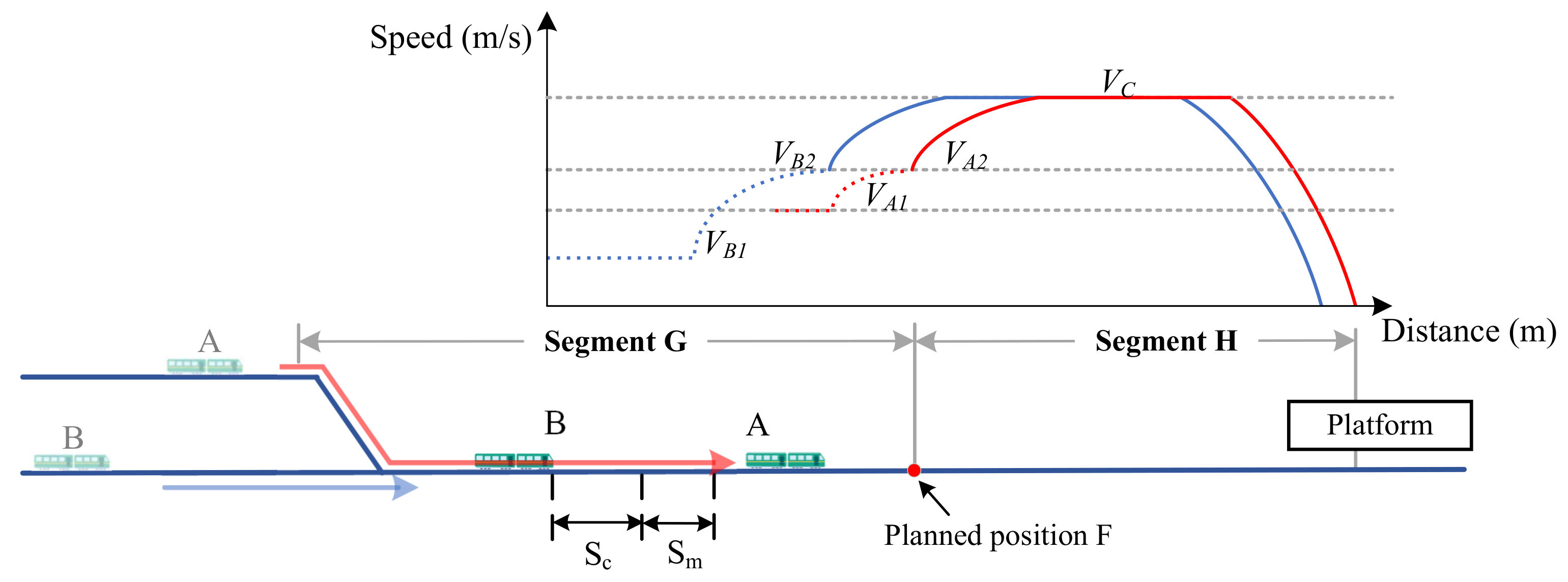
11]. It is urgent to improve the efficiency of the whole travel process. When multiple trains approach a merging junction at the same time, they are prevented from slowing down and/or waiting at the junction until the requested route is fully cleared by previous trains. Train route control is realized by switch control. To guarantee that trains pass switches correctly and safely, switch movements and lock times are set with different speed limits in the normal position and the reverse position.
At junctions, the headways of trains are extended by their absolute braking distances. Trains must reserve large buffer times before switches, resulting in negative effects on the overall travel time. Train operation strategies along continuous routes are discrete. Discrete optimization problem has the non-convex property. Thus, the derivative method cannot solve this problem. In fact, it is difficult to find optimal strategies in a reasonable amount of time. Different control strategies and different initial states remarkably influence the overall coupling efficiency, which makes train coupling a complex process.
To adapt actual control conditions, variable parameters and optimal control strategies are necessary to realize dynamic and efficient control. Braune et al. designed a novel variable engine valve actuator to meet the requirements of high dynamic and low power consumption [12]. Train control is complex, it requires dynamic analyses and adjustment [13]. When merging at junctions, train statuses can be different. Trains must reach a coupled state within the specified distance. The operation strategies for every train concern the entire coupling process. Thus, traditional fixed operation strategies cannot fit the actual situation well. Static pre-programmed strategies may fail to reach the coupled state given a certain initial train speed or line distance.
Game theory is an economical approach for solving multi-participant decision-making problems. It considers both the predicted and actual behaviors of each participant [14]. Game theory includes non-cooperative and cooperative approaches. The former pursues individual profits, while the latter achieves superior total profit through coalition-based cooperation [15]. Cooperative game theory is successfully used in the control of automated vehicles to make decisions and select appropriate improvement strategies [16].
Yang et al. [15] proposed a non-signalized intersection driving model using cooperative game theory and the Shapley allocation method. Liu et al. [17] proposed a spacing allocation method for vehicular platoons using cooperative game theory and the Shapley values to allocate the spacings fairly. With the gradual deepening of virtual coupling research, it is feasible to regard autonomous trains in a convoy as rational participants. Therefore, game theory will become a practicable method to determine optimal operation strategies.
To solve the virtual coupling-based optimization problem at merging junctions, this paper proposes a novel cooperative game-based method for the coupling process. Train control is realized by discrete control command, which is reflected in different acceleration. To optimize the entire coupling process, the proposed model generates control strategies for trains. The strategy is composed of acceleration in every discrete segment point. Decision-making and the overall and allocation costs of the formed alliance are considered in a cooperative game. The objective of the model is to realize a quick formation and increase the synchronous moving speed of the convoy. It orients the entire train operation control to the coupling process at junctions. The Shapley value is used to allocate the cost of a train coalition.
The cooperative game model can generate different optimal strategies for participants according to specific scenes. Compared to the continuous problem, the train operation strategies in this model are discrete, which is reflected in the dimensionality of the optimization problem. The computational complexity scales exponentially with the problem size. It is difficult for a cooperative game model to solve large-scale problems within a reasonable time frame in practice [18].
In recent years, many studies have attempted to combine complicated optimization problems with cooperative game models. Vehicle platooning control is closely connected with game theory. Bui et al. [19] proposed a cooperative game theoretic approach and a distributed merging and splitting algorithm to improve traffic flows in large networks. Meng et al. [20] proposed a multi-colony collaborative ant optimization algorithm based on a cooperative game mechanism and applied it to robot path planning.
Liu et al. [21] proposed an intelligent train control method based on the DQN algorithm. Ding et al. [22] aimed at the reconfiguration problem of a distribution network, proposed a multi-objective model based on cooperative game theory, and applied the firefly algorithm to determine the final reconfiguration scheme. The above research shows that characterizing multi-vehicle collaborative control relationships through cooperation and competition has broad prospects. Since its introduction in 1995 [23], particle swarm optimization (PSO) has been successfully used in many optimization problems.
Yet, the basic PSO algorithm has several shortcomings. Two of the major failure modes are stagnation and convergence to local optima [24]. Many studies (such as [25,26]) have been carried out to relieve and solve this problem. To achieve better performance, PSO is combined with other intelligent algorithms, such as differential evolution [27,28], ant colony optimization [29,30,31], and genetic algorithms [32,33,34].
Adaptive methods are also used for refining the coefficient values of PSO [35,36,37]. There are several challenges faced by the basic PSO algorithm when fitting a cooperative model. The discrete control characteristic is reflected in the particle dimension. Operating conditions are reflected in the constraints of the fitness function in PSO.
Thus, to apply a game model in general scenarios, we introduce an improved particle swarm optimization (PSO) approach to solve the strategy decision problem of the game model. To improve the efficiency of solving a cooperative model with large dimensions and complicated constraints, we modify the conventional PSO algorithm in the following aspects. A search speed limit factor and a speed bound are used to prevent solution explosion and limit the maximum and minimum particle movement speeds. Adaptive penalty functions are used to effectively measure the degrees of constraint violations. A no-update method is used to prevent particles from exceeding the search boundary. The mutation algorithm mentioned in [38] is also used in the improved PSO approach. This helps PSO to enhance population diversity and avoid the local optima problem.
The aim of this work is to propose a novel solution in the field of railways for virtual coupling trains at junctions. The method can realize a quick formation and increase the synchronous moving speed of the convoy and, thus, improve the efficiency of virtual coupling. The cooperative game theorem is used to abstract the coupling process into a concrete model, and the improved PSO is used to find the optimal operation strategies for every train.
The contributions of this paper are as follows. A novel optimization approach for virtual coupling, which aims to improve the coupling efficiency of trains at junctions on the run, is proposed. A game theory-based model is built to represent the strategy decision-making behavior of each train. An improved PSO algorithm is developed to enable the game model to solve larger-scale problems. The proposed approach is applied to a typical coupling scenario. Contrast tests are carried out to compare the proposed optimization approach with two naive control strategies and the unimproved PSO approach. The results show that the coupling efficiency is improved with the proposed optimal operation strategies.
The rest of the paper is organized as follows. Section 2 presents the problem of merging at junctions, builds a dynamic model for virtual coupling, and discretizes the model. Section 3 builds a cooperative model and defines several of its important elements. Section 4 proposes the improved PSO approach and explains the detailed algorithm. Section 5 shows the simulation scenario and the comparative results of several operation methods. Section 7 concludes the paper.

2. Problem Statement

A coupling process before arriving at a station and the resulting coupled state are shown in Figure 1. In this process, automated control trains are regarded as agents of the system that influence the behavior of the group [17]. This section presents the two main states of virtual coupling: the coupling state and the coupled state.

2.1. Coupling State

The requirements and conditions of virtual coupling are checked momentarily. When trains satisfy the coupling conditions, neighboring trains begin to adjust their speeds and distances to reach the final coupled state. In segment G of Figure 1, train A and train B merge at a junction and couple to a convoy. These two trains are coupled at the planned position F.
Their initial speeds are V A 1 and V B 1 , respectively. V A 2 and V B 2 are their speeds at the end of the coupling process. V A 2 and V B 2 are equal to the synchronous coupling speed V C . The running distances of train A and train B are S A and S B , respectively. Their running speeds are V A and V B , respectively. S c is the initial coordinate distance in the coupling process. The distance between train A and train B is S c + S m . At the end of the coupling process, the distance between trains decreases to S m .
The safety margin S m depends on the train speeds, the velocity error V δ , the vehicle-vehicle communication time T 1 , the data processing time T 2 , and the length of the predecessor L k . The calculation of S m is executed as follows:
S m = ( ( V B + V δ ) ( V A V δ ) ) × ( T 1 + T 2 ) L k

2.2. Coupled State

In the coupled state, successive trains run synchronously. Cooperative train operation is equivalent to the automatic train operation (ATO) strategy of existing train control systems. It is used to guarantee the stability of the platoon.
Segment H in Figure 1 shows the coupled running statuses of two trains. The trains are in a relatively stable state. The following train maintains the minimum safety distance to the preceding train and conducts cooperative control with it. In the coupled state, the speeds of train A and train B are approximately the same. S t h is the permissible distance error with respect to S m , and V t h is the permissible distance error with respect to the coupled speed V A or V B . The running distance and speed satisfy the following constraints:
S A S B S m [ S t h , S t h ]
V A V B [ V t h , V t h ]
Virtual coupling-based train protection is closely related to cooperative train operation; however, they are two completely different train operation control concepts. Virtual coupling protection uses the relative braking distance to space trains in a coupled convoy. Cooperative train operation controls trains in a convoy and guarantees the stability of the convoy.
In a convoy, the tracking interval between two neighboring trains is computed according to the relative braking distance. This distance depends on the following factors [4]:
  • the braking characteristic of the following train;
  • the braking characteristic of the preceding train;
  • the absolute accelerations, speeds and distances of the two neighboring trains; and
  • the relative accelerations, speeds and distances of the two neighboring trains.
Let R B D be the relative braking distance, B D f be the braking distance of the following train, and B D p be the braking distance of the preceding train. The R B D of the trains is as follows:
R B D = S m , B D f B D p
R B D = B D f B D p + S m , B D f > B D p
If the braking distance of the following train is shorter than or equal to the preceding train’s braking distance, R B D takes the minimum value in (4). Otherwise, R B D takes the value in (5). R B D in (4) means that if two coupled trains have the same braking characteristics, the braking distance is the same. Thus, the spacing distance between them can be reduced to the minimum safety distance S m .

2.3. Dynamic Model

The dynamic train model that we utilize is based on longitudinal train dynamics (LTD) [7]. Trains are regarded as mass points in this model, as mentioned in [39,40]. A dynamic model is introduced to describe the dynamic behavior of virtual coupling trains, which can be described as follows:
x ˙ = f t ( x , u )
where x represents the state of the train, f t denotes the mapping relationship presents in (9) to (12); x = [ s , v , a ] T ; the variables s (m), v (m/s), and a (m/s2) represent the position, speed, and acceleration of the train, respectively; and u is the driving or braking force. Let T be the traction force, F d s be the service braking force, and F b r be the braking resistance due to pneumatic braking [7]. When the train is running with traction, u can be calculated by (7); otherwise, when the train is braking, u can be calculated by (8):
u = T , t r a i n i s r u n n i n g w i t h t r a c t i o n .
u = F d s F b r , t r a i n i s b r a k i n g .
Let M ( k g ) be the mass of the train, R ( v , ϕ , c ) ( N ) be the resultant resistance (which depends on the speed v, gradient ϕ , and radius of curvature c), F ( N ) be the resultant tractive or braking force, and τ be the inertial lag of longitudinal dynamics. Equation (6) can be calculated in detail as follows:
s ˙ = v
v ˙ = a
M · a = u R ( v , ϕ , c )
a ˙ = u F τ × M
The acceleration a satisfies the following constraint:
a [ a b , a d ]
where a b is the maximum braking deceleration and a d is the maximum driving acceleration. To apply these dynamics in the remainder of this paper, we discretize them with the state updating Equations (14) and (15).
x [ η + 1 ] = f ( x [ η ] , u [ η ] )
f ( x [ η ] , u [ η ] ) = f ( x [ η ] ) + Δ t × f t ( x [ η ] , u [ η ] )
where η ( s ) is the time instant and Δ t ( s ) is the sample time.

3. Cooperative Game Model Design

This paper mainly studies the coupling process of trains. Every autonomous train gathers information from other trains or ground equipment through frequent communication. These trains can be regarded as agents; they can judge conditions and make decisions throughout the whole process. The control behaviors influence each other in a system. Therefore, it is rather difficult to analyze the interactions among agents in theory.
We use a cooperative game to model the confrontation and cooperation of agents in virtual coupling control. Cost functions describe the tasks of all agents. The goal of solving this model is to obtain a set of strategies, thereby, minimizing the entire cost (or maximizing the entire payoff) of the game. This section introduces the cooperative game model, defines the cost function of the game, and then uses the Shapley theorem to solve it.

3.1. Strategy Set

The running statuses of trains depend on the operation strategies in this model. Let S be the strategy set of the cooperative model. S k = [ a k 1 , a k 2 , , a kj , ] denotes the strategy set of train k, which can be described as a two-dimensional acceleration matrix:
S k = [ [ a 1 ( x 1 ) , a 1 ( x 2 ) , , a 1 ( x j ) , , a 1 ( x l ) ] [ a 2 ( x 1 ) , a 2 ( x 2 ) , , a 2 ( x j ) , , a 2 ( x l ) ] [ a i ( x 1 ) , a i ( x 2 ) , , a i ( x j ) , , a i ( x l ) ] ]
where a ki = [ a i ( x 1 ) , a i ( x 2 ) , , a i ( x j ) , , a i ( x l ) ] is the ith strategy for train k, which is composed of acceleration at every segment point. a i ( x j ) represents the acceleration of segment point j in a ki . a i can be any value in [ a m i n , a m a x ] , in which a m i n is the lower bound of the acceleration and a m a x is the upper bound of the acceleration. The train state x can be calculated using Equations (14) and (15).
In a game, n virtual coupling trains are participants, and train k has l k distance segments. Thus, the strategy dimensionality of train i is l k . As the value of the acceleration in each segment can be infinitely large, the strategy set of each participant can be infinitely large.
The task of the cooperative game model is to match strategies from every train and calculate the overall cost function f c . It is difficult to find the optimal solution of this problem within a reasonable time frame. Therefore, a search algorithm is required for this model. The improved PSO algorithm is discussed in the next section.

3.2. Cooperative Game Model and the Cost Functions

This study considers the selection of a control strategy for every train in the coupling process as a cooperative game model. n coupling trains in a platoon correspond to n participants in a game. The game can be described as < N , f c > . The participant set N = { 1 , 2 , 3 , , i , , n } , i denotes participant i. The entire cost function of the coalition is f c . Let P be a coalition consisting of participants from the coalition. P N is a subset of N. The total cost of coalition P can be denoted as f c ( P ) . Let i, j, k be trains i, j and k, respectively.
The coalition can be expressed as , { i | i N } , { i , j | i , j N , i j } , { i , j , k | i , j , k N , i j k } , …, N = { 1 , 2 , 3 , , n } We make the following assumptions and abstract the coupling process into a cooperative game model.
  • The cooperators in a coalition can benefit from the game only when the number of participants is greater than 2; otherwise, the cost function is positive infinity. f c [ ] = + , f c [ { i } ] = + .
  • After passing the switches in the coupling process, the order in which the trains are arranged is fixed. This means that a train in a convoy or platoon cannot skip its predecessor. Thus, the coalition can only take in the form of a queue { 1 , 2 } , { 1 , 2 , 3 } , …, { 1 , 2 , 3 , , k , , n 1 , n } . The cost functions of other coalition forms are positive infinity.
  • The cost functions of this problem consist of three parts: a formation time, a running speed, and the summed extra interval distance to the predecessor in a coupled platoon.
The cost functions f c ( P ) are the main goals of each agent or the coalition. The compositions of f c ( P ) are as follows.
For a coupled platoon, let D j , k be the distance between train j and train k. The distance difference cost f c d ( j , k ) of the convoy is defined as follows:
f c d ( j , k ) = D j , k S m
Let v k be the running speed of train k, the speed cost f c v 1 ( k ) can be described as follows:
f c v 1 ( k ) = v k v δ
Let Δ v j , k be the speed difference between train j and train k, the speed difference cost f c v 2 ( k ) can be described as follows:
f c v 2 ( j , k ) = Δ v j , k + v δ
Let t k be the running time of train k. For phase of trains before the switch, the time cost function f c t 1 ( k ) is as follows:
f c t 1 ( k ) = t 1 k
After passing the switch, the time cost function f c t 2 ( k ) is as follows:
f c t 2 ( k ) = t 2 k
Function Γ 1 transforms the distance to time:
Γ 1 ( f c d ( j , k ) ) = f c d ( j , k ) v k
Function Γ 2 transforms train speed to time:
Γ 2 ( f c v 1 ( k ) ) = 2 × D b r a k i n g f c v 1 ( k )
where D b r a k i n g denotes the required distance for braking. Let λ 1 , λ 2 , λ 3 , and λ 4 be the distribution weights of the distance cost, speed cost, speed difference cost, and time cost, respectively. They determine the importance levels of these four goals.
The cost function of trains can be divided into two phases. For phase of trains before the switch, the cost function f c 1 is as follows:
f c 1 [ ] = + f c 1 [ { i } ] = + f c 1 [ { i , j } ] = λ 4 · f c t 1 ( i ) + λ 4 · f c t 1 ( j ) f c 1 [ { i , j , k } ] = λ 4 · f c t 1 ( i ) + λ 4 · f c t 1 ( j ) + λ 4 · f c t 1 ( k ) f c 1 [ N ] = λ 4 · k = 1 n f c t ( k )
Let L i , j be the distance between train i and train j, L j , k be the distance between train j and train k, L k , k 1 be the distance between train k and train k 1 , and w = ( 1 , 2 , 3 , , n ) be the train sequence. The cost function f c 2 of the phase of train beyond the switch is as follows.
f c 2 [ ] = + f c 2 [ ( i ) ] = + f c 2 [ ( i , j ) ] = λ 2 · Γ 2 ( f c v 1 ( i ) ) + λ 2 · Γ 2 ( f c v 1 ( j ) ) + λ 4 · f c t 2 ( i ) + λ 4 · f c t 2 ( j ) + λ 1 · Γ 1 ( f c d ( i , j ) ) + λ 3 · f c v 2 ( i , j ) , L i , j > 0 f c 2 [ ( i , j , k ) ] = λ 2 · Γ 2 ( f c v 1 ( i ) ) + λ 2 · Γ 2 ( f c v 1 ( j ) ) + λ 2 · Γ 2 ( f c v 1 ( k ) ) + λ 4 · f c t 2 ( i ) + λ 4 · f c t 2 ( j ) + λ 4 · f c t 2 ( k ) + λ 1 · Γ 1 ( f c d ( i , j ) ) + λ 1 · Γ 1 ( f c d ( j , k ) ) + λ 3 · f c v 2 ( i , j ) + λ 3 · f c v 2 ( j , k ) , L i , j > 0 a n d L j , k > 0 f c 2 [ w ] = k = 1 n λ 2 · Γ 2 ( f c v 1 ( k ) ) + k = 1 n λ 4 · f c t 2 ( k ) + k = 1 n 1 λ 1 · Γ 1 ( f c d ( k , k + 1 ) ) + k = 1 n 1 λ 3 · f c v 2 ( k , k + 1 ) , k > 1 , L k , k 1 > 0
where L i , j > 0 denotes that train i is always the leading train. Let f c 2 be + when L i , j 0 . The values of λ 1 , λ 2 , λ 3 , and λ 4 are considered as 1 in this paper, but they can be different according to different requirements. For the phase of trains beyond the switch, the total cost function is the sum of f c 1 and f c 2 :
f c = f c 1 + f c 2

3.3. Solution of the Cooperative Game

Given sets P 1 and P 2 , we denote P 1 \ P 2 to be set P 1 minus set P 2 . The marginal cost f m ( P , k ) = f m 1 ( P , k ) of the phase of trains before the switch is as follows.
f m 1 ( P , k ) = f c ( P ) f c ( P \ { k } )
According to (24), f m 1 ( P , k ) is as follows:
f m 1 ( P , k ) = λ 4 · f c t 1 ( k )
Given a sequence w , we define w | k to be the removing of an element k from w . The margin cost f m ( P , k ) = f m 2 ( P , k ) of the phase of trains beyond the switch is as follows.
f m 2 ( P , k ) = f c ( P ) f c ( P | k )
According to (25), f m 2 is as follows:
f m 2 ( P , k ) = λ 2 · Γ 2 ( f c v 1 ( k ) ) + λ 4 · f c t 2 ( k ) + λ 1 · Γ 1 ( f c d ( k , k 1 ) ) + λ 3 · f c v 2 ( k , k 1 )
At the end of the coupling process, the marginal cost function is the sum of cost functions in two phases:
f c m ( P , k ) = λ 2 · Γ 2 ( f c v 1 ( k ) ) + λ 4 · f c t 1 ( k ) + λ 4 · f c t 2 ( k ) + λ 1 · Γ 1 ( f c d ( k , k 1 ) ) + λ 3 · f c v 2 ( k , k 1 )
The cost distribution scheme is the preparatory phase of cooperation. We use Shapeley values to distribute coalition costs. For participant i, the cost is apportioned by the following equation:
Φ k ( f c ) = P N \ k ψ · f c m ( P , k )
ψ = θ ! ( n θ 1 ) ! n !
where θ denotes the participants number in coalition P and ψ is the probability for θ to form a specific coalition.
Let g r be the r constraint of the problem and m be the total number of constraints. The solution of the cooperative game is to minimize the cost function f c ( P ) , as shown in (34) and (35):
m i n f c ( P )
s . t . g γ 0 , γ = 1 , 2 , 3 , , m
Formula (35) represents all constraints of the game model. The minimized cost function is the optimization of the final coupled convoy, which has smaller running intervals, better synchronism and a faster speed than other platoons. The constraints of the model in (35) are as follows:
a i ( x j ) [ a m i n , a m a x ]
v i ( x s ) < v l s n o r v i ( x s ) < v l s r
v ( 0 , v m a x )
Δ t k , k 1 ( x s ) ( t l s , + )
The parameters are shown in Table 1.

4. The Improved Particle Swarm Optimization Algorithm

Particle swarm optimization (PSO) is widely used for practical optimization problems. In our cooperative game model, the scale is large, the constraints are complicated, and the basic PSO algorithm performs poorly on this problem. To solve the above issues, this paper improves upon the basic PSO algorithm and fits it to the model. The objective of this algorithm is to minimize the cost function of the coalition, which is described in (34).
The improved PSO algorithm aims to minimize the objective function f c ( P ) . Taking the constraints into consideration, we transform this problem into an unconstrained problem. Let ϕ ( P ) be the penalty function and f i t n e s s ( P ) be the fitness function of the algorithm, which can be described as follows:
f i t n e s s ( P ) = f c ( P ) + ϕ ( P )
The penalty function consists of the constraints in (35). An adaptive penalty function is designed to prevent the penalty function from being too large or too small:
ϕ ( P ) = ϵ ( β ) × γ = 1 m m a x ( g γ , 0 )
The penalty coefficient ϵ is defined as follows:
ϵ ( β ) = 10 α ( 1 β )
where β is the ratio of the number of feasible solutions to the number of total solutions in an iteration and α is an adjustable parameter. The penalty is adaptive according to the ratio of feasible solutions. Thus, the constrained problem becomes an unconstrained problem.
In this model, the particle dimension is vast, and bound constraints are imposed on every dimension of each particle. The conventional PSO algorithm easily falls into local optima under these conditions. In addition, the efficiency of the algorithm is confined. To address these deficiencies, we improve the algorithm in the following ways. To prevent solution explosion caused by a search speed that is too fast, we add a speed limit factor ζ [ 0 , 1 ] to the iterative formula:
V p q + 1 = ζ ( ω V p q + c 1 r p 1 q ( P p q X p q ) + c 2 r p 2 q ( P g q X p q ) )
X p q + 1 = X p q + V i q + 1
The meanings of the variables in the above two equations are explained in Table 2.
To increase the search efficiency of the algorithm, we add a search speed constraint V m a x to reduce the possibility of a particle being out of range. The value range of V is as follows:
V [ V m a x , V m a x ]
We add judgment to the search process. If the particle exceeds the basic position constraint, we use the last position to replace the current position. The basic PSO algorithm usually cannot strike a balance between its global searching ability and local search ability. To overcome this shortcoming, this paper uses the self-adapting inertia weight ω proposed in [38]:
ω = ω m a x I * ω m a x ω m i n I m a x
where w m a x is the maximum inertia weight, w m i n is the minimum inertia weight, I is the current number of iterations, and I m a x is the maximum number of iterations.
In the iterative process, if a particle is in the current best position, other particles draw close to it quickly. If it is a local optima, the particle swarm no longer searches in the solution space. Thus, the algorithm falls into this local optima. According to (43) and (44), the next position of the particle swarm depends on the original search speed, the optimal particle fitness, and the global optimal fitness. The search speed can be changed if we change the global optimal fitness through a mutation algorithm; therefore, the search direction of the particle swarm changes. It is possible for the algorithm to find new optimal particle fitness and global optimal fitness values.
This paper uses the mutation algorithm mentioned in [38]. Let f i be the fitness of particle i and f a v e be the average fitness of the particle swarm; the group fitness variance σ 2 describes the aggregation degree of the particle swarm, as follows:
σ 2 = i = 1 n ( f i f a v g f ) 2
where f is the normalized calibration factor, which can be calculated as follows:
f = m a x { | f i f a v g | } , m a x { | f i f a v g | } > 1 1 , o t h e r s
The group fitness variance σ 2 represents the aggregation degree of the particle swarm. The smaller it is, the more the swarm is aggregated. Otherwise, the swarm is more dispersed.
If the swarm gathers too early, the algorithm stagnates in a local optima solution. This causes the algorithm to exhibit low efficiency or even fail. Within the maximum number of iterations, the global optimal fitness mutates as a mutation probability P m to increase the population diversity.
P m = k , σ 2 < σ d 2 a n d f ( P g ) > f d 0 , o t h e r s
where k is a random value in [ 0.1 , 0.3 ] ; σ d 2 is related to the actual conditions and is much lower than the maximum value of σ 2 . f d can be set to a small value; thus, the optimal fitness moves to this value.
The mutation of P g adopts the stochastic disturbance approach. Let P g k be the kth dimension of P g and η g be a random number obeying a Gaussian [ 0 , 1 ] distribution; the mutated P g k is as follows:
P g k = P g k · ( 1 + 0.5 * η g )
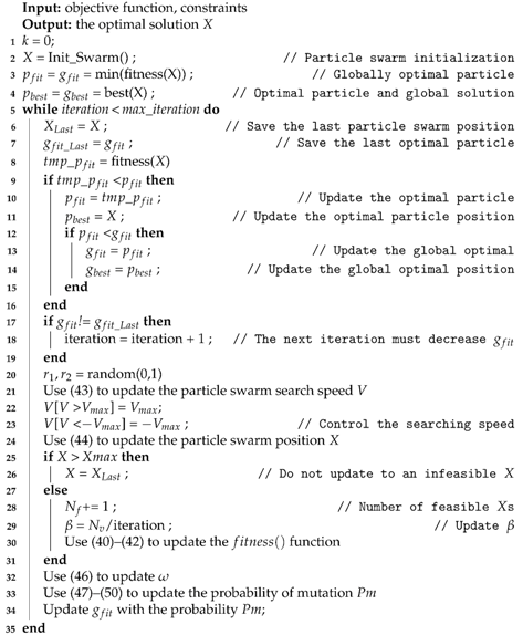
The improved PSO algorithm can adaptively adjust the parameters according to the solution conditions. The algorithm is shown in Algorithm 1.
Algorithm 1: Improved PSO Algorithm
Actuators 10 00207 i001

5. Simulation

5.1. Simulation Environment

The virtual coupling process is simulated in this section, where trains start running from different tracks to verify the effect of the proposed approach. Three coupling approaches are compared, including the game-based approach and two naive approaches, where naive strategy 1 lets the trains closest to the switch pass it first and then has the trains keep moving according to limit speed of the switch, and naive strategy 2 lets the fastest trains pass the switch first and then has the trains keep moving according to the limit speed of the switch. Let the train with faster speed pass the switch at first.
To validate the efficiency differences between these several approaches, we simulate a representative scenario in Figure 2. Train 1, train 2, and train 3 are three coupling trains from three tracks their initial speeds are v 1 , v 2 , and v 3 , respectively. S 1 , S 2 , and S 3 are the distances to switch 1 or switch 2 from the three trains, respectively. S 4 is the distance between switch 1 and switch 2. S 5 is the distance from switch 2 to the planned coupled position. The trains form platoons and synchronously arrive at the platform. Different initial conditions are set and compared.

5.2. Simulink Results

Three scenarios, which have different initial distances and speeds, are set as shown in Table 3.
The simulation of naive strategy 1 in scenario 1 is shown in Figure 3, in which (a) shows speed–time curves and (b) shows distance–time curves of three trains. The expected sequence is train 3, train 2, and train 1. In this scenario, train 3 with a short distance passes switch 1 and switch 2 first, train 2 waits at the switches until train 3 passes, and train 1 waits at the switches until train 2 passes. The results show that the initial train reaches the expected planned coupled position, while the following train does not reach switch 2. Finally, the trains fail to reach the coupled state at the expected position.
The simulation of naive strategy 2 in scenario 1 is shown in Figure 4, in which (a) shows speed–time curves and (b) shows distance–time curves of three trains. The expected sequence is train 1, train 3, and train 2. In this scenario, train 1 with a faster speed passes switch 2 first; train 2 and train 3 have the same speed, and the train closer to the switch has priority. Train 2 wait at the switches until train 3 passes. The result is similar to that of naive strategy 1 in scenario 1. Finally, the trains fail to reach the coupled state at the expected position.
The simulation of the unimproved PSO strategy in scenario 2 is shown in Figure 5, in which (a) shows operation strategies and (b) shows speed–time curves of three trains. Only one of the running results is shown. In the actual experiment, the unimproved PSO algorithm may fall into local optima or stagnate in an infeasible solution and cause the algorithm to fail. Finally, the trains fail to reach the coupled state at the expected position.
The simulation of the improved PSO strategies in scenarios 1, 2, and 3 are shown in Figure 6, Figure 7 and Figure 8, in which (a) shows the operation strategies and (b) shows speed–time curves of three trains. In scenario 1, the coupling time is 57.8 s, the coupled speed is 15.6 m/s, and the cost function value is 180.1. In scenario 2, the coupling time is 77.5 s, the coupled speed is 14.7 s, and the cost function value is 230.5. In scenario 3, the coupling time is 68.2 s, the coupled speed is 15.7 m/s, and the cost function value is 211.1.
According to different initial states, the algorithm generates corresponding operation strategies for every train. The platoon formed by the improved PSO algorithm has a faster coupling speed and a shorter stabilization time than the unimproved PSO algorithm. By using a cooperative game model and the improved PSO algorithm, the trains couple at the expected position quickly. Furthermore, the coupling speed is relatively fast.

6. Discussions

We compare train operation results with trains using different operation strategies in different scenarios. The results of the simulation show that the proposed train operation strategy generation method was effective to couple train at junctions in the planned distance. Compared with the proposed optimization method, the two naive pre-programmed operation strategies lack flexibility. Trains have to wait before the switch according to the naive strategy. This will cause extra times for operations of virtual coupled trains. In fact, in most cases, trains are not able to be coupled at the planned coupled position with the naive strategy.
Compared with the proposed optimization method, the unimproved PSO easily falls into local optima and results in the failure of the algorithm. Trains have very small probabilities of being coupled at the planned position. It is difficult for the algorithm to find an optimal solution and guarantee the final coupled state.
Thus, the improved PSO is necessary to solve the cooperative game-based model and generate optimal operation strategies. The proposed method aims to guarantee the final coupled status of trains. In addition, this method maximizes the coupled speed of the convoy and minimizes the coupling time of the overall process.

7. Conclusions and Future Works

In this paper, we addressed the problem of optimal operation control strategies for virtual coupling trains at junctions. First, we formulated a cooperative game-based model for the coupling process as an optimal problem. Then, the cost function was formulated. The game was solved by minimizing the cost function of the coalition. Finally, we designed an improved PSO to find the optimal solution of the model and generate strategies for trains.
The proposed method was validated through simulation and then compared with two pre-programmed train operation strategies and the unimproved PSO strategies generating method. The proposed method can generate different operation strategies for every train according to specific conditions. Compared with the two naive strategies, the proposed method reached coupled status in the planned position. It is almost impossible for the naive strategies to reach the coupled status within such a short distance. Compared with the unimproved PSO strategies generating method, the proposed method can better adapt the cooperative game model and obtain an optimal solution. Nevertheless, the unimproved PSO strategy demonstrated great contingency and easy convergence to local optima. This can cause extra waiting time or even failure of the coupling process.
Furthermore, the proposed method demonstrated shorter coupling times. Compared with naive strategy 1, naive strategy 2, and the unimproved PSO strategy, it decreased train operation time by 41.7%, 22.10%, and 54.85%, respectively. The proposed method also had a faster coupled speed. Compared with naive strategy 1, naive strategy 2, and the unimproved PSO strategy, it increased train operation speed by 4.2%, 6.3%, and 63.08%, respectively.
Future research should attempt to extend the virtual coupling optimization to a multi-object problem. Energy conservation and comfort should be considered for better passenger experience and environmental protection.

Author Contributions

Conceptualization, Q.W. and M.C.; methodology providing, H.L.; formal analysis, T.T.; writing—original draft preparation, Q.W.; writing—review and editing, M.C.; data analysis, T.T.; validation, H.L. All authors have read and agreed to the published version of the manuscript.

Funding

This research was funded by the Fundamental Research Funds for the Central Universities under grant 2019JBM002.

Conflicts of Interest

The authors declare no conflict of interest.

References

  1. Mitchell, I.; Goddard, E.; Montes, F.; Stanley, P.; Muttram, R.; Coenraad, W.; Poré, J.; Andrews, S.; Lochman, L. ERTMS level 4 train convoys or virtual coupling. IRSE News 2016, 219, 14–15. [Google Scholar]
  2. Quaglietta, E.; Wang, M.; Goverde, R.M. A multi-state train-following model for the analysis of virtual coupling railway operations. J. Rail Transp. Plan. Manag. 2020, 15, 100195. [Google Scholar] [CrossRef]
  3. Quaglietta, E. Analysis of platooning train operations under v2v communication-based signaling: Fundamental modelling and capacity impacts of virtual coupling. In Proceedings of the 98th Transportation Research Board Annual Meeting, Washington, DC, USA, 13–17 January 2019. [Google Scholar]
  4. Shift2Rail. Application Roadmap for the Introduction of Virtual Coupling; MOVINGRAIL, European: Maastricht, The Netherlands, 2020; pp. 1–74. [Google Scholar]
  5. Shift2Rail. Virtual Coupling Communication Solutions Analysis; MOVINGRAIL, European: Maastricht, The Netherlands, 2020; pp. 1–63. [Google Scholar]
  6. Goikoetxea, J. Roadmap towards the wireless virtual coupling of trains. In International Workshop on Communication Technologies for Vehicles; Springer: Berlin/Heidelberg, Germany, 2016; pp. 3–9. [Google Scholar]
  7. Felez, J.; Kim, Y.; Borrelli, F. A model predictive control approach for virtual coupling in railways. IEEE Trans. Intell. Transp. Syst. 2019, 20, 2728–2739. [Google Scholar] [CrossRef]
  8. Schumann, T. Increase of capacity on the Shinkansen high-speed line using virtual coupling. In Proceedings of the COMPRAIL 2016, Madrid, Spain, 19–21 July 2016. [Google Scholar]
  9. Su, S.; Wang, X.; Cao, Y.; Yin, J. An Energy-Efficient Train Operation Approach by Integrating the Metro Timetabling and Eco-Driving. IEEE Trans. Intell. Transp. Syst. 2020, 21, 4252–4268. [Google Scholar] [CrossRef]
  10. Su, S.; Tang, T.; Xun, J.; Cao, F.; Wang, Y. Design of Running Grades for Energy-Efficient Train Regulation: A Case Study for Beijing Yizhuang Line. IEEE Intell. Transp. Syst. Mag. 2021, 13, 189–200. [Google Scholar] [CrossRef]
  11. Aoun, J.; Quaglietta, E.; Goverde, R.M. Investigating market potentials and operational scenarios of virtual coupling railway signaling. Transp. Res. Rec. 2020, 2674, 799–812. [Google Scholar] [CrossRef]
  12. Braune, S.; Liu, S.; Mercorelli, P. Design and control of an electromagnetic valve actuator. In Proceedings of the 2006 IEEE Conference on Computer Aided Control System Design, 2006 IEEE International Conference on Control Applications, 2006 IEEE International Symposium on Intelligent Control, Munich, Germany, 4–6 October 2006; pp. 1657–1662. [Google Scholar] [CrossRef]
  13. Chai, M.; Wang, H.; Tang, T.; Liu, H. Runtime verification of train control systems with parameterized modal live sequence charts. J. Syst. Softw. 2021, 177, 110962. [Google Scholar] [CrossRef]
  14. Quan, B.; Lu, X.; Zhang, Y.; Mou, Z. A Multi-objective Tracking Task Assignment Algorithm Based on Game Theory. J. Phys. 2021, 1802, 032115. [Google Scholar]
  15. Yang, Z.; Huang, H.; Wang, G.; Pei, X.; Yao, D.Y. Cooperative driving model for non-signalized intersections with cooperative games. J. Cent. South Univ. 2018, 25, 2164–2181. [Google Scholar] [CrossRef]
  16. Basiri, M.H.; Pirani, M.; Azad, N.L.; Fischmeister, S. Security of vehicle platooning: A game-theoretic approach. IEEE Access 2019, 7, 185565–185579. [Google Scholar] [CrossRef]
  17. Liu, Y.; Zong, C.; Han, X.; Zhang, D.; Zheng, H.; Shi, C. Spacing Allocation Method for Vehicular Platoon: A Cooperative Game Theory Approach. Appl. Sci. 2020, 10, 5589. [Google Scholar] [CrossRef]
  18. DUAN, G.R. High-order system approaches: I. fully-actuated systems and parametric designs. Acta Autom. Sin. 2020, 46, 1333–1345. [Google Scholar]
  19. Bui, K.H.N.; Jung, J.J. Cooperative game-theoretic approach to traffic flow optimization for multiple intersections. Comput. Electr. Eng. 2018, 71, 1012–1024. [Google Scholar]
  20. Meng, L.; You, X.; Liu, S. Multi-Colony Collaborative Ant Optimization Algorithm Based on Cooperative Game Mechanism. IEEE Access 2020, 8, 154153–154165. [Google Scholar] [CrossRef]
  21. Liu, W.; Su, S.; Tang, T.; Wang, X. A DQN-based intelligent control method for heavy haul trains on long steep downhill section. Transp. Res. Part C Emerg. Technol. 2021, 129, 103249. [Google Scholar] [CrossRef]
  22. Ding, Y.; Wang, F.; Bin, F.; Zhou, W. Multi-objective distribution network reconfiguration based on game theory. Electr. Power Autom. Equip. 2019, 2. [Google Scholar] [CrossRef]
  23. Kennedy, J.; Eberhart, R. Particle swarm optimization. In Proceedings of the ICNN’95-International Conference on Neural Networks 1995, Perth, Australia, 27 November–1 December 1995; Volume 4, pp. 1942–1948. [Google Scholar]
  24. Sengupta, S.; Basak, S.; Peters, R.A. Particle Swarm Optimization: A survey of historical and recent developments with hybridization perspectives. Mach. Learn. Knowl. Extr. 2019, 1, 157–191. [Google Scholar] [CrossRef] [Green Version]
  25. Li, C.; Yang, S.; Nguyen, T.T. A self-learning particle swarm optimizer for global optimization problems. IEEE Trans. Syst. Man Cybern. Part B (Cybern.) 2011, 42, 627–646. [Google Scholar]
  26. Hossen, M.S.; Rabbi, F.; Rahman, M.M. Adaptive Particle Swarm Optimization (APSO) for multimodal function optimization. Int. J. Eng. Technol. 2009, 1, 98–103. [Google Scholar]
  27. Huo, J.; Ma, L.; Yu, Y.; Wang, J. Hybrid algorithm based mobile robot localization using DE and PSO. In Proceedings of the 32nd Chinese Control Conference, Xi’an, China, 26–28 July 2013; pp. 5955–5959. [Google Scholar]
  28. Seyedmahmoudian, M.; Rahmani, R.; Mekhilef, S.; Oo, A.M.T.; Stojcevski, A.; Soon, T.K.; Ghandhari, A.S. Simulation and hardware implementation of new maximum power point tracking technique for partially shaded PV system using hybrid DEPSO method. IEEE Trans. Sustain. Energy 2015, 6, 850–862. [Google Scholar] [CrossRef]
  29. Niknam, T.; Amiri, B. An efficient hybrid approach based on PSO, ACO and k-means for cluster analysis. Appl. Soft Comput. 2010, 10, 183–197. [Google Scholar] [CrossRef]
  30. Lazzus, J.; Rivera, M.; Salfate, I.; Pulgar-Villarroel, G.; Rojas, P. Application of particle swarm+ ant colony optimization to calculate the interaction parameters on phase equilibria. J. Eng. Thermophys. 2016, 25, 216–226. [Google Scholar] [CrossRef]
  31. Mandloi, M.; Bhatia, V. A low-complexity hybrid algorithm based on particle swarm and ant colony optimization for large-MIMO detection. Expert Syst. Appl. 2016, 50, 66–74. [Google Scholar] [CrossRef]
  32. Yu, S.; Wei, Y.M.; Wang, K. A PSO–GA optimal model to estimate primary energy demand of China. Energy Policy 2012, 42, 329–340. [Google Scholar] [CrossRef]
  33. Abdel-Kader, R.F. Genetically improved PSO algorithm for efficient data clustering. In Proceedings of the 2010 Second International Conference on Machine Learning and Computing, Bangalore, India, 12–13 February 2010; pp. 71–75. [Google Scholar]
  34. Garg, H. A hybrid PSO-GA algorithm for constrained optimization problems. Appl. Math. Comput. 2016, 274, 292–305. [Google Scholar] [CrossRef]
  35. Ratnaweera, A. Particle swarm optimization with self-adaptive acceleration coefficients. In Proceedings of the International Conference on Fuzzy Systems & Knowledge Discovery (FSKD 2002), Singapore, 18–22 November 2002; Volume 1, pp. 264–268. [Google Scholar]
  36. Clerc, M. The Way of Life Cheap-pso, an Adaptive Pso. In Proceedings of the IEEE Congress on Evolutionary Computation, San Francisco, CA, USA, 16–19 July 2000; Volume 3, pp. 1951–1957. [Google Scholar]
  37. Shi, Y.; Eberhart, R.C. Fuzzy adaptive particle swarm optimization. In Proceedings of the 2001 Congress on Evolutionary Computation (IEEE Cat. No. 01TH8546), Seoul, Korea, 27–30 May 2001; Volume 1, pp. 101–106. [Google Scholar]
  38. Lu, Z.S.; Hou, Z.R. Particle swarm optimization with adaptive mutation. Acta Electron. Sin. 2004, 32, 416–420. [Google Scholar] [CrossRef]
  39. Iwnicki, S. Handbook of Railway Vehicle Dynamics; CRC Press: Boca Raton, FL, USA, 2006. [Google Scholar]
  40. Wu, Q.; Spiryagin, M.; Cole, C. Longitudinal train dynamics: An overview. Veh. Syst. Dyn. 2016, 54, 1688–1714. [Google Scholar] [CrossRef]
Figure 1. Coupling and coupled states of train A and train B.
Actuators 10 00207 g001
Figure 2. “Coupled point” to “Coupling point” Simulink scenario.
Actuators 10 00207 g002
Figure 3. Trains operation curves of naive strategy 1 in scenario 1.
Actuators 10 00207 g003
Figure 4. Trains operation curves of naive strategy 2 in scenario 1.
Actuators 10 00207 g004
Figure 5. Unimproved PSO strategies and operation curves in scenario 2.
Actuators 10 00207 g005
Figure 6. Improved PSO strategies and operation curves in scenario 1.
Actuators 10 00207 g006
Figure 7. Improved PSO strategies and operation curves in scenario 2.
Actuators 10 00207 g007
Figure 8. Improved PSO strategies and operation curves in scenario 3.
Actuators 10 00207 g008
Table 1. List of parameters in constraints.
ParameterMeaningValue
a i ( x j ) acceleration of train i in segment j [ a m i n , a m a x ] (m/s2)
a m i n lower bound of acceleration−1.2 (m/s2)
a m a x upper bound of acceleration1 (m/s2)
x s segment number of the switch position1
v l s n limit speed of the switch in the normal position15 (m/s)
v l s r limit speed of the switch in the reverse position10 (m/s)
vtrain speed ( 0 , v m a x ) (m/s)
v m a x limit speed of the whole segment G20 (m/s)
t l s minimum transfer time of the switch10 (s)
Δ t k , k 1 ( x s ) time difference between train k and train k 1 when passing switch ( t l s , + ) (s)
Table 2. Parameter settings in the iterative formula.
Variable NamesMeanings
qIteration times
pNumber of particles
VSearch speed
wInertia weight
c 1 Cognitive constant
c 2 Social constant
r 1 , r 2 Normally distributed random numbers
P p Optimal particle fitness
P g Global optimal fitness
XParticle positions
Table 3. The distances and speeds of three scenarios.
Scenarios S 1 ( m ) S 2 ( m ) S 3 ( m ) S 4 ( m ) S 5 ( m ) v 1 ( m / s ) v 2 ( m / s ) v 3 ( m / s )
1400200160200200201515
2600400200200200102010
34002002002002005510
Publisher’s Note: MDPI stays neutral with regard to jurisdictional claims in published maps and institutional affiliations.

