Observer-Based Coordinated Control for Blended Braking System with Actuator Delay

Abstract

The coordinated control of a blended braking system is always a difficult task. In particular, blended braking control becomes more challenging when the braking actuator has an input time-delay and some states of the braking system cannot be measured. In order to improve the tracking performance, a coordinated control system was designed based on the input time-delay and state observation for a blended braking system comprising a motor braking system and friction braking system. The coordinated control consists of three parts: Sliding mode control, a multi-input single-output observer, and time-delay estimation-based Smith Predictor control. The sliding mode control is used to calculate the total command braking torque according to the desired braking performance and vehicle states. The multi-input single-output observer is used to simultaneously estimate the input time-delay and output braking torque of the friction braking system. With time-delay estimation-based Smith Predictor control, the friction braking system is able to effectively track the command braking torque of the friction braking system. The tracking of command braking torque is realized through the coordinated control of the motor braking system and friction braking system. In order to validate the effectiveness of the proposed approach, numerical simulations on a quarter-vehicle braking model were performed.

1. Introduction

With rising concerns over global environmental and energy issues, the automotive industry has started to focus on electric vehicles (EVs) in recent years since they have the advantages of zero emissions and high efficiency. However, the driving range of EVs is limited compared with fuel vehicles. The regenerative braking system is capable of effectively improving energy efficiency by converting the vehicle’s kinetic energy into electric energy during braking procedures. Studies show that in urban driving situations, about one-third to one-half of the energy of the power plant is consumed during the deceleration process [1,2,3]. Regenerative braking has become a popular area of research for improving the energy efficiency of EVs [4]. Due to the limited braking torque of a regenerative braking system, a friction braking system is still needed to ensure the vehicle’s braking performance. Thus, most vehicles adopt a blended braking system.

Compared with the conventional friction braking system, the blended braking system is able to recover energy and responds quickly. However, in contrast to the conventional friction braking system, the blended braking system comprises different braking systems with quite different dynamic characteristics. For example, the motor’s brake torque responds quickly and accurately. The blended braking system has three different braking states: Friction braking, motor braking, and hybrid braking. These three braking states may occur independently or frequently alternate during one braking procedure [5,6,7]. The coordinated control of the blended braking system is a difficult task.

For commercialized EVs with motor braking, the braking torque distribution is based on the braking situation. When the vehicle enters an emergency braking situation, the motor braking torque is removed quickly, and the friction braking system completely takes over the ABS control [5,6]. The cooperative control of motor braking and friction braking during the normal braking process has also attracted wide attention and inspired many studies [7,8,9,10,11,12,13,14]. When the vehicle enters a normal braking situation, the motor braking torque and friction braking torque are distributed according to a certain proportion [6,7]. The cited studies do not take the dynamics of braking actuators into consideration. However, the dynamics of actuators have a significant effect on the stability of vehicle braking control and should not be ignored.

The effect of the flexibility of an electric drivetrain on the blended brake control performance was analyzed in [15,16]. Blended braking control algorithms with compensation for the powertrain flexibility were developed using an extended Kalman filter. The output braking torque of the friction braking system was estimated by the extended Kalman filter. However, the input time-delay was not taken into consideration in [15,16]. In [17], the sliding mode control and an optimal braking torque distribution strategy were proposed. For the braking torque distribution, the dynamics of the motor braking system and friction braking system were analyzed. However, the output braking torque of the friction braking system and input time-delay were treated as measurable and known [17]. In fact, these two parameters are hard to obtain directly in real applications.

In friction braking systems, such as the hydraulic braking system, there is a gap between the actuator and the brake disc. This gap increases with the wear of materials, which changes the input time-delay of the friction braking system. Thus, the input time-delay of the friction braking system must be estimated. In addition, the output braking torque of the friction braking system cannot be directly measured in the blended braking system. To the best of the authors’ knowledge, no research has reported the simultaneous observation of the input time-delay and output braking torque of a friction braking system in a blended braking system. There are some research papers on the time-delay and state observer design [18,19,20]. However, they focus on the disturbance [19] and single-input single-output (SISO) system [20]. This approach is not suitable for the blended braking system since blended braking is a multi-input single-output system.

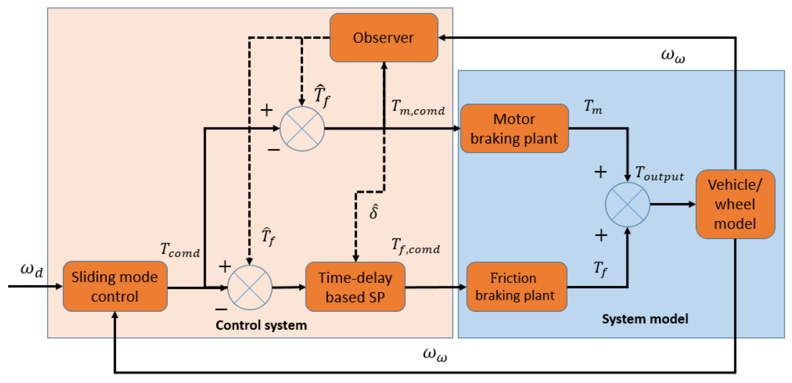
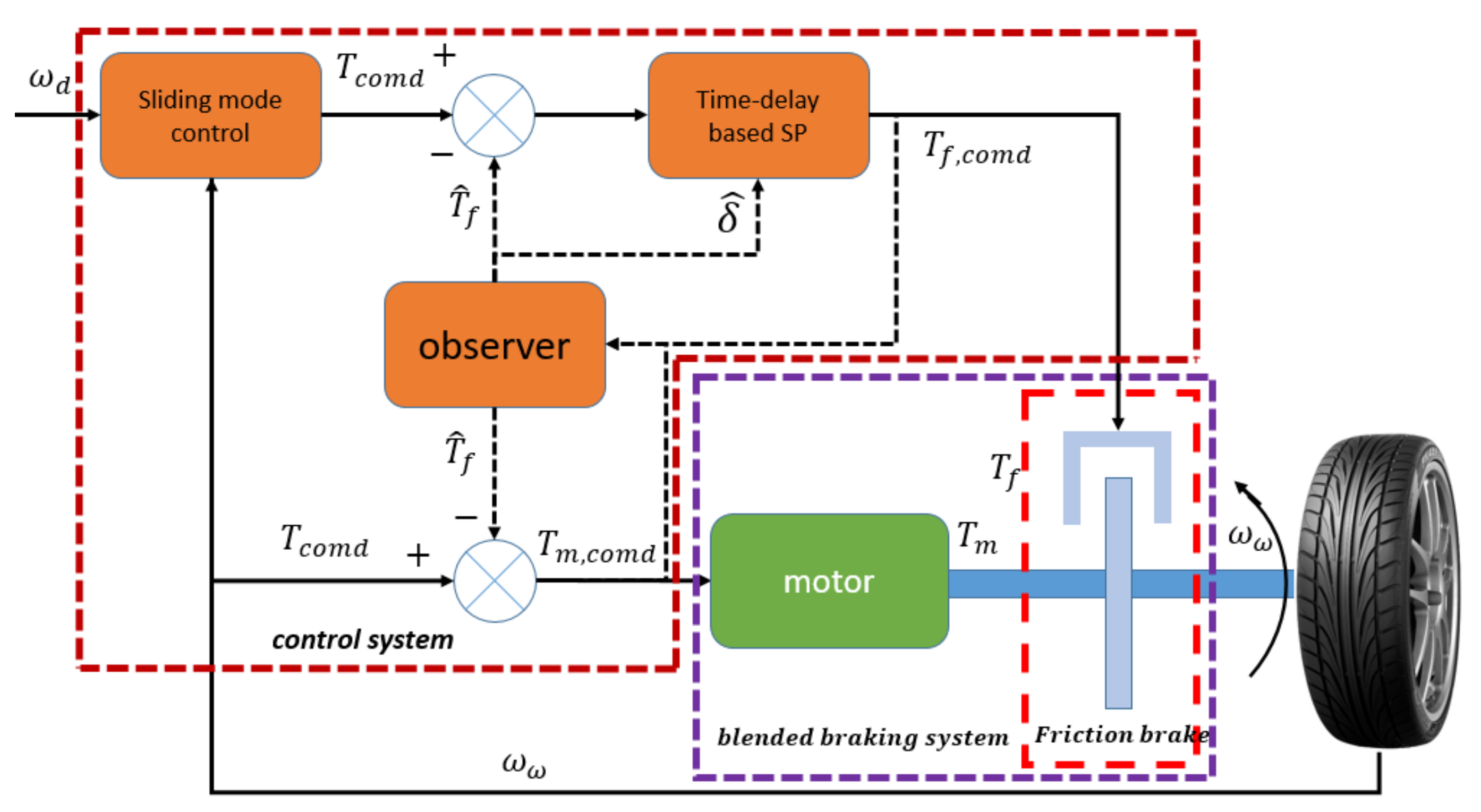
The main contributions of this paper are three-fold. First, an observer is designed for the blended braking system. The observer is able to simultaneously estimate the output braking torque and input time-delay of the friction braking system in the blended braking system. Second, the time-delay-based Smith Predictor control is implemented in the friction braking system. The last contribution is the new blended braking system control structure. It makes full use of the advantages of sliding mode control (i.e., strong anti-interference and rapid response), the motor braking system (i.e., fast response speed), and the friction braking system (i.e., large braking torque). As a result, the blended braking system is able to effectively track the desired braking performance.

The remaining sections of this paper are organized as follows. First, the system model is introduced, including models of quarter-vehicle dynamics, motor braking dynamics, and friction braking dynamics. Second, the braking control strategy is introduced. The braking control strategy includes sliding mode control to achieve the desired braking performance, an observer to estimate the input time-delay and output braking torque of the friction braking system, and time-delay estimation-based Smith Predictor control for the friction braking system control. Then, the simulation results are presented. Finally, conclusions are provided in the last section.

2. Vehicle Model

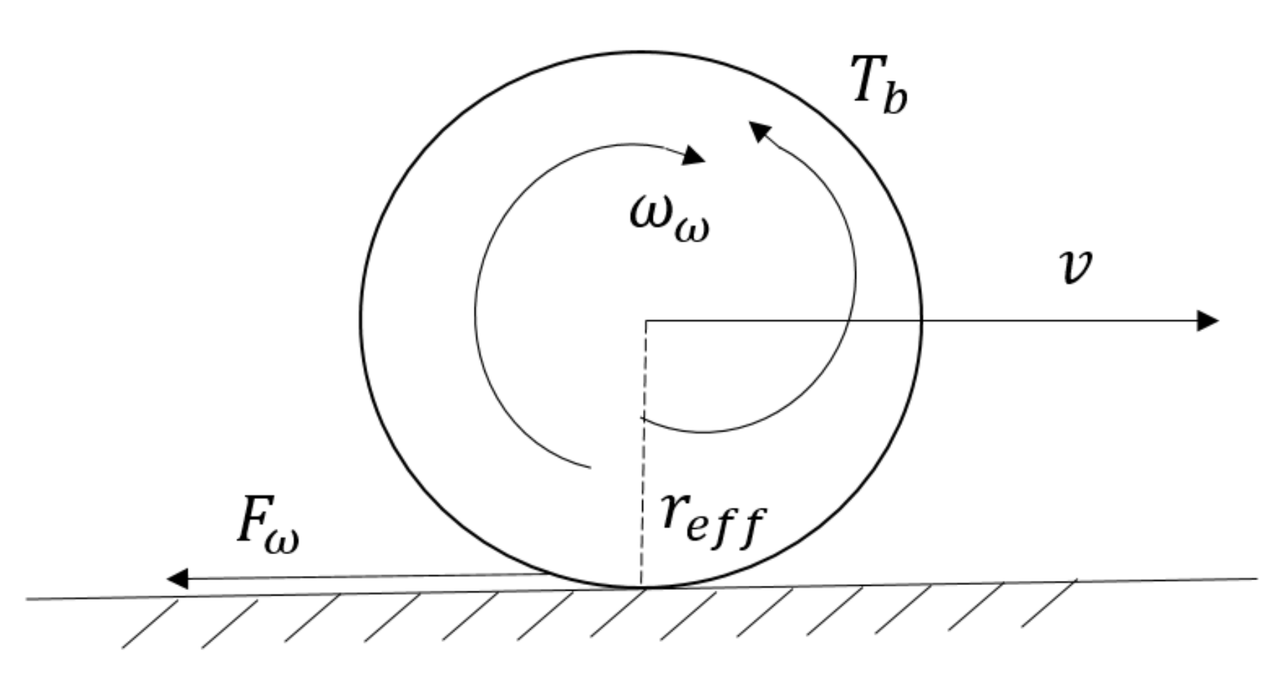
In this paper, the braking system of each independently controlled wheel is treated as a research object. For convenience, a quarter-vehicle model is adopted. The quarter-vehicle model, which is simple but effective (see Figure 1), is used, and only the longitudinal force is considered in this paper.

The quarter-vehicle blended braking system is shown in Figure 2. As shown in Figure 2, each wheel is equipped with a blended braking system: A motor braking system and a friction braking system.

In this paper, the normal braking situation is analyzed. During the normal braking process, the wheel slip is small and can be ignored. Then, the rotational speeds of the four wheels are equal, and the relationship between the wheel speed and vehicle velocity can be written as:

$$v={\omega }_{\omega }{r}_{eff}$$

(1)

where $v$ is the vehicle speed, ${\omega }_{\omega }$ is the wheel speed, and $r_{eff}$ is the wheel radius. The vehicle speed control can be converted to wheel speed control. In order to achieve vehicle speed control through wheel speed control, the motion inertia of the vehicle should be converted to that of the wheel [21]. According to the law of conservation of energy, the equivalent moment of inertia can be obtained:

$$\frac{1}{2}J{\omega }_{\omega }^2=\frac{1}{2}m{v}^2+\frac{1}{2}{J}_{\omega }{\omega }_{\omega }^2$$

(2)

where $J$ is the equivalent moment of inertia, $m$ is the mass of the quarter-vehicle, and $J_{\omega }$ is the moment of inertia of the wheel. Then, the equivalent moment of inertia can be obtained:

$$J=m{r}_{eff}^2+J_{\omega }$$

(3)

Then, the dynamics control of the quarter vehicle can be converted to the dynamics control of the wheel (as shown in Figure 2). The dynamics of the wheel can be expressed by the following equations:

$$J{\dot{\omega }}_{\omega }=-T_b-r_{eff}{F}_{\omega }$$

(4)

$$T_b=T_f+T_m$$

(5)

$$F_{\omega }=f_{v}mg{\omega }_{\omega }$$

(6)

where $T_b$ is the total braking torque acting on the wheel, $T_f$ is the output braking torque of the friction braking system, $T_m$ is the output braking torque of the motor braking system, $F_{\omega }$ is the wheel viscous friction force, $f_v$ is the wheel viscous friction coefficient, and $g$ is the gravitational acceleration. When the driver makes a braking action, the desired vehicle braking deceleration can be converted to the desired wheel braking deceleration according to the following equation:

$${\dot{\omega }}_d=\frac{{\dot{v}}_d}{r_{eff}}$$

(7)

where ${\dot{v}}_d$ is the desired vehicle deceleration speed, and ${\dot{\omega }}_d$ is the desired wheel deceleration. According to the desired vehicle deceleration speed and the initial braking speed of the vehicle, the desired vehicle speed can be obtained. Then, the desired wheel speed can be calculated.

As shown in Figure 2, the blended braking system comprises a motor braking system and friction braking system. Regarding the effect of the electric system dynamics, the motor braking system can be modeled as a first-order reaction, with a short time constant ${\tau }_m$ being taken into consideration [22]. It can be expressed as follows:

$$T_m=\frac{T_{m,comd}}{{\tau }_{m}s+1}$$

(8)

where $T_m$ is the output braking torque of the motor braking system, $T_{m,comd}$ is the command braking torque of the motor braking system, and ${\tau }_m$ is the time constant of the motor braking system. In the friction braking system, there is a gap between the brake disc and the brake actuator. When the command braking torque is released, the brake actuator has an empty stroke. The braking torque response is approximated by a first-order system with a time delay [22]:

$$T_f=\frac{T_{f,comd}}{{\tau }_{f}s+1}{e}^{-\delta s}$$

(9)

where $T_{f,comd}$ is the command braking torque of the friction braking system, $T_f$ is the output braking torque of the friction braking system, ${\tau }_f$ is the dominant time constant of the friction braking system, and $\delta$ is the pure time-delay. The relevant parameters are listed in

Table 1. System parameters.

Symbol	Property	Value
$m$	Mass of quarter-vehicle	$365 \mathrm{kg}$
$J_{\omega }$	Moment of inertia of the wheel	$1 {\mathrm{kg}*\mathrm{m}}^2$
$J$	Equivalent moment of inertia	$33.85{ \mathrm{kg}*\mathrm{m}}^2$
$r_{eff}$	Wheel radius	$0.3 \mathrm{m}$
$f_v$	Wheel viscous friction coefficient	$0.012$
${\tau }_m$	Time constant of motor	$0.01$
${\tau }_f$	Time constant of friction braking system	$0.4$
$C_1$	Positive constant	$5$
$\eta$	Positive constant	$5$
$\overline{\delta }$	Time bound	2 s
$g$	Gravitational acceleration	$9.8 \mathrm{m}/{\mathrm{s}}^2$
$\rho$	Positive constant	$1000$
$P$	PID control	2
$I$	PID control	2
$T_{m,max}$	Maximum braking torque of motor	$100 Nm$

.

3. Braking Control

The whole control structure is shown in Figure 3 and Figure 4. As shown in Figure 3, the outermost layer adopts the sliding mode control, which is used to ensure that the wheel speed tracks the desired speed. The command braking torque can be calculated through the sliding mode controller.

Each braking system has its own characteristics. Compared with the motor braking system, the friction braking system can provide a larger braking torque. The motor braking system has a faster response than the friction braking system. In order to make full use of the advantages of the respective braking system, the command braking torque is used as the input of the friction braking system, and the difference between the command braking torque and the output braking torque of the friction braking system is used as the command braking torque of the motor braking system. The friction braking system can provide the majority of the command braking torque, and the motor braking system can compensate for the slow response of the friction braking system. As a result, the blended braking system is able to obtain effective tracking performance. In order to obtain the fastest possible friction braking response, time-delay estimation-based Smith Predictor (SP) control is adopted. However, neither the output braking torque nor the input time-delay of the friction braking system can be directly measured. In order to solve this problem, an observer is designed. The observer is able to estimate the input time-delay and output braking torque of the friction braking system simultaneously. The details about the controller and observer are introduced in the next part. Since the motor has a fast response and the motor usually has a special controller, the motor torque controller design is not considered in this paper.

3.1. Wheel Speed Control

According to Equation (7), the desired vehicle deceleration speed and desired vehicle speed can be achieved through the wheel deceleration speed and speed control. In this paper, it is assumed that the wheel speed can be measured and that the wheel viscous friction coefficient is known. Due to the influence of actuator dynamics (the motor braking system is a first-order system, and the friction braking system is a first-order system with an input time-delay), the command braking torque of actuators cannot be achieved in time [23]. The difference between the command braking torque of the actuators $\left(T_{comd}\right)$ and the output braking torque of the actuators $\left(T_m+T_f\right)$ varies with the change in the command braking torque and the change in the braking torque distribution between the different braking actuators. The difference between the command braking torque and output braking torque of the actuators can be regarded as disturbance and is denoted by $\mathsf{\Delta }$. It is assumed that $\left|\mathsf{\Delta }\right|\le {\mathsf{\Delta }}_{max}$. ${\mathsf{\Delta }}_{max}$ is the boundary of disturbance. Then, the command braking torque can be represented as $T_{comd}=T_m+T_f-\mathsf{\Delta }$. Thus, Equation (4) can be rewritten as follows:

$$J{\dot{\omega }}_{\omega }=-\left(T_{comd}+\mathsf{\Delta }\right)-r_{eff}{f}_{v}mg{\omega }_{\omega }$$

(10)

Equation (10) can also be rewritten as:

$${\dot{\omega }}_{\omega }=-\frac{T_{comd}}{J}-\frac{r_{eff}{f}_{v}mg}{J}{\omega }_{\omega }-{\mathsf{\Delta }}_J$$

(11)

where ${\mathsf{\Delta }}_J=\frac{\mathsf{\Delta }}{J}$, $\left|{\mathsf{\Delta }}_J\right|\le \frac{{\mathsf{\Delta }}_{max}}{J}$. As shown in Equation (10), the influence of the actuator dynamics (there is a difference between command braking torque and the real output braking torque acting on the wheel) can be regarded as disturbance. The sliding mode control has a fast response and can effectively resist disturbance, so it is chosen as the controller. In order to design the sliding mode control, the sliding mode surface should be selected first, and it is defined as:

$$S_1={\omega }_{\omega }-{\omega }_d$$

(12)

$${\dot{S}}_1={\dot{\omega }}_{\omega }-{\dot{\omega }}_d$$

(13)

The desired wheel deceleration is related to the brake pedal travel. When the braking pedal travel and the initial braking speed are given, the desired wheel deceleration and desired wheel speed can be calculated. The braking torque control is designed according to the following equation:

$$T_{comd}=J(-\frac{r_{eff}{f}_{v}mg{\omega }_{\omega }}{J}-{\dot{\omega }}_d+C_1\left({\omega }_{\omega }-{\omega }_d\right)+\eta sgn\left(S_1\right))$$

(14)

where $C_1$ and $\eta$ are both positive constants.

The Lyapunov function is expressed as:

$${\mathrm{V}}_1=\frac{S_1^2}{2}$$

(15)

Then, (11), (12), (13), and (14) are substituted into the derivative of Equation (15). The derivative of Equation (15) can be obtained as follows:

$${\dot{\mathrm{V}}}_1=S_1{\dot{S}}_1=-C_1{S}_1^2-\eta \left|S_1\right|-{\mathsf{\Delta }}_J{S}_1$$

(16)

where $\eta \ge \frac{{\mathsf{\Delta }}_{max}}{J}$, ${\dot{\mathrm{V}}}_1\le 0$ and $\underset{t\to \infty }{\lim }{\omega }_{\omega }={\omega }_d$. Then, the wheel is able to track the desired wheel speed, and the vehicle is able to track the desired vehicle speed. This also means that the vehicle can realize the desired deceleration.

3.2. Friction Braking System Observer Design

The time constant of the motor braking system ${\tau }_m$ and the time constant of the friction braking system ${\tau }_f$ can be obtained from the technical manual or measured in advance. The output braking torque of the motor braking system can be easily calculated or measured [24]. In this paper, it is assumed that the time constants of the motor braking system and friction braking system are known.

However, the input time-delay of the friction braking system $\delta \left(t\right)$ is influenced by many factors. It may change and is hard to measure or know in advance. Thus, the output braking torque of the friction braking system is hard to measure and cannot be calculated directly. In this paper, a new observer is designed to estimate the output braking torque and input time-delay of the friction braking system. In order to design the observer, Equations (4), (8), and (9) can be rewritten as the following equations:

$${\dot{\omega }}_{\omega }=-\frac{\left(T_f+T_m\right)}{J}-\frac{r_{eff}{f}_{v}mg}{J}{\omega }_{\omega }$$

(17)

$${\dot{T}}_m=\frac{-T_m}{{\tau }_m}+\frac{u_1}{{\tau }_m}$$

(18)

$${\dot{T}}_f=\frac{-T_f}{{\tau }_f}+\frac{u_2\left(t-\delta \left(t\right)\right)}{{\tau }_f}$$

(19)

where $u_1=T_{m,comd};u_2=T_{f,comd}$. Then, the vehicle dynamic model with actuators (Equations (17)–(19)) can be rewritten as the following state equations:

$$\dot{x}=Ax+BU$$

(20)

$$y=Cx\left(t\right)=x_1$$

(21)

where $x={\left[\begin{array}{ccc}{x}_1& x_2& x_3\end{array}\right]}^{’}$ and $x_1={\omega }_{\omega };x_2=T_m;x_3=T_f$; $A=\left[\begin{array}{ccc}-\frac{r_{eff}{f}_{v}mg}{J}& -\frac{1}{J}& -\frac{1}{J}\\ 0& \frac{-1}{{\tau }_m}& 0\\ 0& 0& \frac{-1}{{\tau }_f}\end{array}\right];B=\left[\begin{array}{cc}0& 0\\ \frac{1}{{\tau }_m}& 0\\ 0& \frac{1}{{\tau }_f}\end{array}\right];C=\left[\begin{array}{ccc}1& 0& 0\end{array}\right];U=\left[\begin{array}{c}{u}_1\\ u_2\left(t-\delta \left(t\right)\right)\end{array}\right].$.

The input time-delay $\delta \left(t\right)$ is unknown and can be time-varying. It is assumed that it is modeled as a continuous and differentiable function that satisfies $\delta \left(t\right)ϵ\left[\begin{array}{cc}0& \overline{\delta }\end{array}\right]; \dot{\delta }\left(t\right)=\psi \left(t\right)$, and $\left|\psi \left(t\right)\right|\le H$ $\overline{\delta }$ and $H$ are the bounds. Taylor’s theorem is used to remove the delay from the control [19]. It is assumed that the input $u_2$ is differentiable. Then, $u_2$ can be written as:

$$u_2\left(t-\delta \left(t\right)\right)=u_2\left(t\right)-\delta \left(t\right){\dot{u}}_2\left(t\right)+\mathsf{{\rm Y}}\left(t-\delta \left(t\right)\right)$$

(22)

where $\mathsf{{\rm Y}}\left(t-h\left(t\right)\right)$ is called the remainder. From Equation (22), the first-order approximation of $u_2\left(t-\delta \left(t\right)\right)$ can be calculated by:

$$u_2\left(t-\delta \left(t\right)\right)\approx u_2\left(t\right)-\delta \left(t\right){\dot{u}}_2\left(t\right)$$

(23)

The accuracy of this calculation increases when $u_2\left(t-\delta \left(t\right)\right)$ is approximated by a higher order. However, from a practical point of view, it was arbitrarily decided to stop at the first order as a tradeoff between problems induced by numerical differentiation and approximation precision. The objective is to design an observer that is able to estimate the input time-delay and output braking torque of the friction braking system simultaneously. Thus, Equation (20) should be reconstructed. According to Equation (23), the input $U$ can be rewritten as:

$$U=\left[\begin{array}{c}{u}_1\\ u_2\left(t-\delta \left(t\right)\right)\end{array}\right]=\left[\begin{array}{c}{u}_1\\ u_2\left(t\right)-\delta \left(t\right){\dot{u}}_2\left(t\right)\end{array}\right]=\left[\begin{array}{c}{u}_1\left(t\right)\\ u_2\left(t\right)\end{array}\right]+\left[\begin{array}{c}0\\ -\delta \left(t\right){\dot{u}}_2\left(t\right)\end{array}\right]=u\left(t\right)+\left[\begin{array}{c}0\\ -\delta \left(t\right){\dot{u}}_2\left(t\right)\end{array}\right]$$

(24)

where $u\left(t\right) =\left[\begin{array}{c}{u}_1\left(t\right)\\ u_2\left(t\right)\end{array}\right]$. The input time-delay of the friction braking system needs to be included in the states in order to estimate its value. Denoting the extended vector by $X={\left[\begin{array}{cc}{x}^T& \delta \end{array}\right]}^T$, an extended system with perturbation is obtained. Then, the extended system state equation can be rewritten in the following form:

$$\dot{X}=\overline{A}X+\overline{B}u\left(t\right)+\mathsf{\Gamma }$$

(25)

$$\mathrm{y}=\overline{C}X$$

(26)

where $\overline{A}=\left[\begin{array}{cc}A& -\overleftrightarrow{B}\\ 0& 0\end{array}\right];\overline{B}=\left[\begin{array}{c}B\\ 0\end{array}\right];\mathsf{\Gamma }=\left[\begin{array}{c}B\left[\begin{array}{c}0\\ \mathsf{{\rm Y}}\left(t-h\left(t\right)\right)\end{array}\right]\\ \delta \left(t\right)\end{array}\right]\overline{C}=\left[\begin{array}{cc}C& 0\end{array}\right]; \overleftrightarrow{B}=-B*\left[\begin{array}{c}0\\ {\dot{u}}_2\left(t\right)\end{array}\right]=-\left[\begin{array}{c}0\\ 0\\ \frac{{\dot{u}}_2\left(t\right)}{{\tau }_f}\end{array}\right]$. It can be seen from (25) that the extended system is free of the input time-delay. The error of approximation $\mathsf{{\rm Y}}$ is regarded as a perturbation in the design of the observer as well as the dynamics of the input time-delay $\delta \left(t\right)$. In order to estimate the input time-delay and output braking torque of the friction braking system, the following assumption should be made: The perturbation $\mathsf{\Gamma }$ does not modify the observability of Equation (25). From Equation (20), it can be seen that the system is observable if and only if:

$${\dot{u}}_2\left(t\right) \ne 0$$

(27)

This is a logical condition since if the input is constant and the input time-delay of the friction braking system has no influence on the system, then it cannot be observed. However, this condition can be relaxed using the notion of persistence defined in [3]. Generally speaking, it allows ${\dot{u}}_2\left(t\right)$ to be eliminated at some time instants without adversely affecting the estimation. Although the input time-delay of the friction braking system will change with the use of the braking system, it can be regarded as an invariable constant in one braking process. During the initial braking stage, the pedal travel changes over time. As a result, the command braking torque changes with time. This means that ${\dot{u}}_2\left(t\right)\ne 0$ during the initial stage of braking. Once the input time-delay of the friction braking system $\delta \left(t\right)$ is estimated, the estimation is finished. The estimated $\delta \left(t\right)$ can be used as the input time-delay of this braking process and can also be transferred to the time-delay-based Smith Predictor (SP) controller. The designed observer is expressed as:

$$\dot{\widehat{X}}=\overline{A}\widehat{X}+\overline{B}u\left(t\right)-S_2^{-1}{\overline{C}}^T\overline{C}\left(\widehat{X}-X\right)$$

(28)

where $\widehat{X}$ is the estimated state. The matrix $S_2$ is the solution of:

$${\dot{S}}_2=-\rho S_2-{\overline{A}}^T{S}_2-S_2\overline{A}+{\overline{C}}^T\overline{C};S_2\left(0\right)>0$$

(29)

where $\rho$ is a positive constant. There exists a real ${\rho }_0$ such that for any symmetric positive definite matrix $S_2\left(0\right)$, for all $\rho \ge {\rho }_0$, there exists $\overline{\alpha }\ge 0, \overline{\beta }\ge 0,$ $t_0>0$ such that for all $t>t_0$:

$$\overline{\alpha }{I}_{n+1}\le S_2\left(t\right)\le \overline{\beta }{I}_{n+1}$$

(30)

The Lyapunov candidate function is expressed as:

$$V_2\left(e\right)=e^T{S}_{2}e$$

(31)

where $e=\widehat{X}-X$. Then, the derivative of $e$ can be written as:

$$\dot{e}=\dot{\widehat{X}}-\dot{X}=\overline{A}\widehat{X}+\overline{B}u\left(t\right)-S_2^{-1}{\overline{C}}^T\overline{C}\left(\widehat{X}-X\right)-\dot{X}$$

(32)

According to the assumption that the perturbation $\mathsf{\Gamma }$ does not modify the observability of Equation (25), Equation (25) can be rewritten as follows:

$$\dot{X}=\overline{A}X+\overline{B}u\left(t\right)$$

(33)

Substituting Equation (33) into (32), $\dot{e}$ can be obtained as follows:

$$\dot{e}=\dot{\widehat{X}}-\dot{X}=\overline{A}\widehat{X}-\overline{A}X-S_2^{-1}R{\overline{C}}^T\overline{C}\left(\widehat{X}-X\right)=(\overline{A}-S_2^{-1}{\overline{C}}^T\overline{C})e$$

(34)

Then, using (29) and (34), the time derivative of $V_2\left(e\right)$ can be written as:

$${\dot{V}}_2\left(e\right)=e^T(-{\overline{C}}^T\overline{C}-\rho S_2)e=-\rho e^T{S}_{2}e-e^T{\overline{C}}^T\overline{C}e$$

(35)

Since $e^T{\overline{C}}^T\overline{C}e\ge 0$,

$$\dot{V}\left(e\right)\le -\rho \overline{\alpha }{\parallel e\parallel }^2$$

(36)

According to Equations (30) and (31), V satisfies the relation:

$$∥\frac{\partial V}{\partial e}∥\le 2\overline{\beta }\parallel e\parallel$$

(37)

Equations (30), (36), and (37) hold globally. According to Lemma 9.4 in [20], positive scalars $k$, $t_0$, $r$, $\theta$ exist such that for all $t\ge t_0$, the following inequality holds:

$$\parallel e\parallel \le k\parallel e\left(t_0\right)\parallel \exp \left(-\theta \left(t-t_0\right)\right)+ r$$

(38)

Equation (38) proves that the estimated states can converge to a ball of radius $r$. The size of $r$ is closely related to the size of the perturbation [19]. Since the perturbation is very small, $\widehat{X}\approx X$.

3.3. Time-Delay Estimation-Based Smith Predictor Controller

The classical control approaches for time-delay systems include proportional–integral–derivative (PID) control and the Smith Predictor. The Smith Predictor aims to design a controller for a time-delay system that results in a delayed response of a delay-free system, as if the time-delay were shifted outside the feedback loop [23]. It is based on the assumption that the controlled object model is known. In addition, the controlled object model is divided into a delay-free part and a pure-delay part. It is assumed that the plant is:

$$G\left(s\right)=P\left(s\right)e^{-\delta s}$$

(39)

where $P\left(s\right)$ is the input time-delay-free part of the controlled object, and $e^{-\delta s}$ is the pure time-delay part of the controlled object. From Equation (9), $P\left(s\right)$ is equivalent to $\frac{1}{{\tau }_{f}s+1}$. $\mathrm{In} \mathrm{addition}, \delta$ is the input time-delay of the friction braking system. The Smith Predictor is realized by introducing local feedback to the main controller $C\left(s\right)$ using the Smith Predictor $Z\left(s\right)$. The Smith Predictor $Z\left(s\right)$ is defined as:

$$Z\left(s\right)=P\left(s\right)-P\left(s\right)e^{-\delta s}$$

(40)

As shown in Equation (40), the Smith Predictor requires the input time-delay of the friction braking system $\delta$. The input time-delay of the friction braking system $\delta$ can be obtained from the observer.

When $P\left(s\right)$ is stable and the input time-delay $\delta$ is known, the Smith Predictor-based control system is as shown in Figure 5. It can be seen from Figure 5 that the input time-delay is now outside of the feedback loop. The main controller $C\left(s\right)$ can be designed according to the input time-delay-free part $P\left(s\right)$ of the model only.

The main controller, $C\left(s\right),$ can only be designed according to the delay-free part $P\left(s\right)$ of the model. The main controller is often designed to meet specified gains and phase margins. For this purpose, a PI controller is adopted. As shown in Figure 5, the transfer function of the closed-loop system can be expressed as:

$$T_{yr}\left(s\right)=\frac{T_f}{T_{f,comd}}=\frac{C\left(s\right)P\left(s\right)e^{-\delta s}}{1+C\left(s\right)P\left(s\right)}$$

(41)

The main controller $C\left(s\right)$ is used for the delay-free part of braking system $P\left(s\right)$ control. The main controller design has to compromise between the robustness and response speed of the system. Thus, the desired delay-free part of the braking system is expressed as: $T_{dyr}\left(s\right)=\frac{1}{{\tau }_{df}s+1}$. The value of ${\tau }_{df}$ can be found in Table 1. According to Equations (9) and (41), in addition to the desired $T_{dyr}\left(s\right)=\frac{1}{0.01s+1}$, the main controller can be calculated as:

$$C\left(s\right)=\frac{0.4s+1}{0.01s}$$

(42)

4. Simulation Results

In this paper, a blended braking system comprising motor braking and friction braking is the research object, of which the related parameters are listed in Table 1.

To the best of the authors’ knowledge, there is little research on an observer that simultaneously estimates the input time-delay and output braking torque of a friction braking system. Therefore, we first tested the designed observer.

As discussed in relation to the wheel speed control, the command braking torque of the motor can be any value, and the derivative of the command braking torque of the friction braking system should not be 0: ${\dot{u}}_2\left(t\right)\ne 0$. In these tests, the command braking torque of the friction braking system is set as a ramp signal: The slope is 10, and the initial value is $0 Nm$. The command braking torque of the motor is a constant number: $10 Nm$. The initial wheel speed is set to $200 rad/s$, the initial braking torque of the friction braking system is $0 Nm$, and the initial braking torque of the motor braking system is $10 Nm$. The initial estimated states are $\widehat{X}=\left[0,0, 0,0.1\right]$, $S\left(0\right)=I_{4*4}$. To test the observer, three groups of simulation experiments were performed.

In the first group of the simulation experiments, the input time-delay is set to a constant value of $0.4 s$. The simulation results are shown in Figure 6a,b.

As shown in Figure 6a,b, the designed observer is able to accurately estimate the input time-delay and the output braking torque of the friction braking system. As shown in Figure 6a, the proposed observer is able to quickly estimate the input time-delay (it is a practical value and is reported as the real time-delay in the simulation results). The output braking torque is 0 during the initial stage (as shown in Figure 6b). This is due to the fact that the actuator has an input time-delay ($0.4 s$). 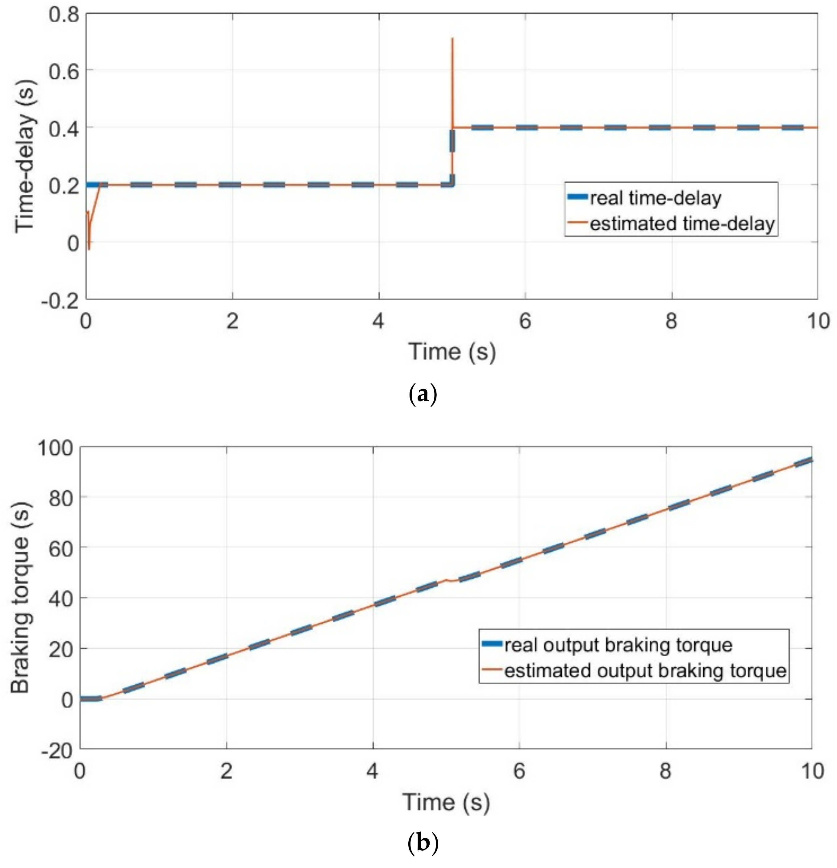This proves that the observer is able to effectively estimate the braking torque of the friction braking system. In order to further verify the effectiveness of the observer and test its estimation ability in the case of a sudden change in the input time-delay parameter, we set up an experiment in which the input time-delay signal is set to 0.2 s for the first 5 and 0.4 s for the subsequent 5 s. The simulation results are shown in Figure 7a,b.

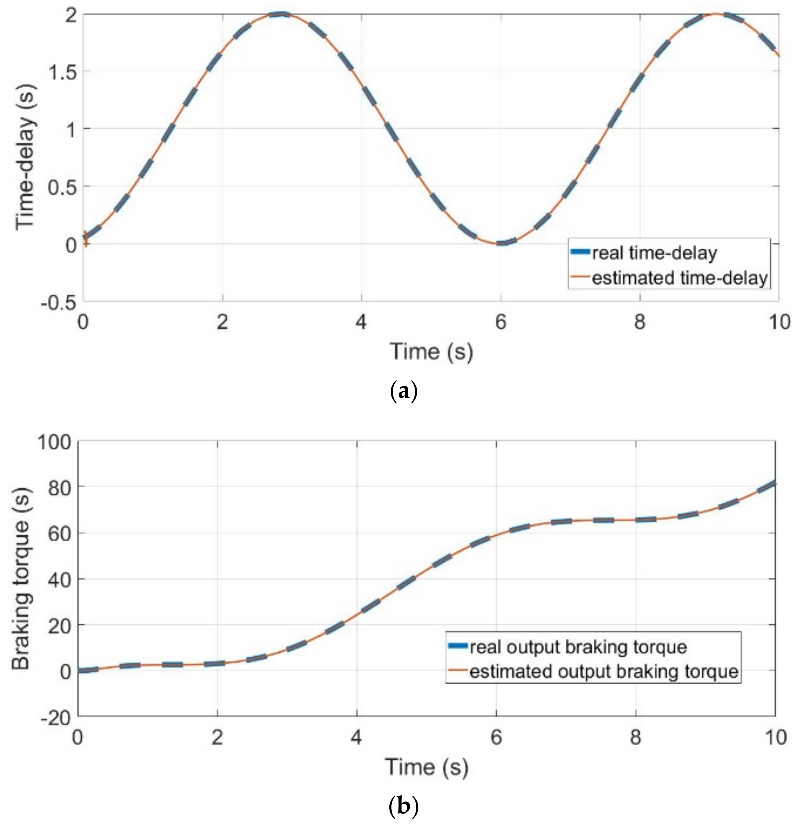
Due to the sudden change in the input time-delay signal, there is an overshoot in the estimated input time-delay at around 5 s. It can be seen from Figure 7a that the designed observer is able to estimate the input time-delay even if the input time-delay changes. Figure 7b proves that the designed observer can accurately estimate the output braking torque of the friction braking system even if the input time-delay changes during the braking process. During the initial stage and at about the fifth second, the braking torque does not change. This is due to the fact that the actuator has a time delay, and the input time-delay changes at the fifth second. To further verify the effectiveness of the observer, the input time-delay signal is set to a sinusoidal signal. The simulation results are shown in Figure 8a,b.

As shown in Figure 8a,b, the observer is able to estimate the input time-delay and output braking torque of the friction braking system, even if the input time-delay signal changes with time as a sinusoidal signal. All of these tests prove that the designed observer is able to effectively estimate the input time-delay and output braking torque of the friction braking system in many different situations.

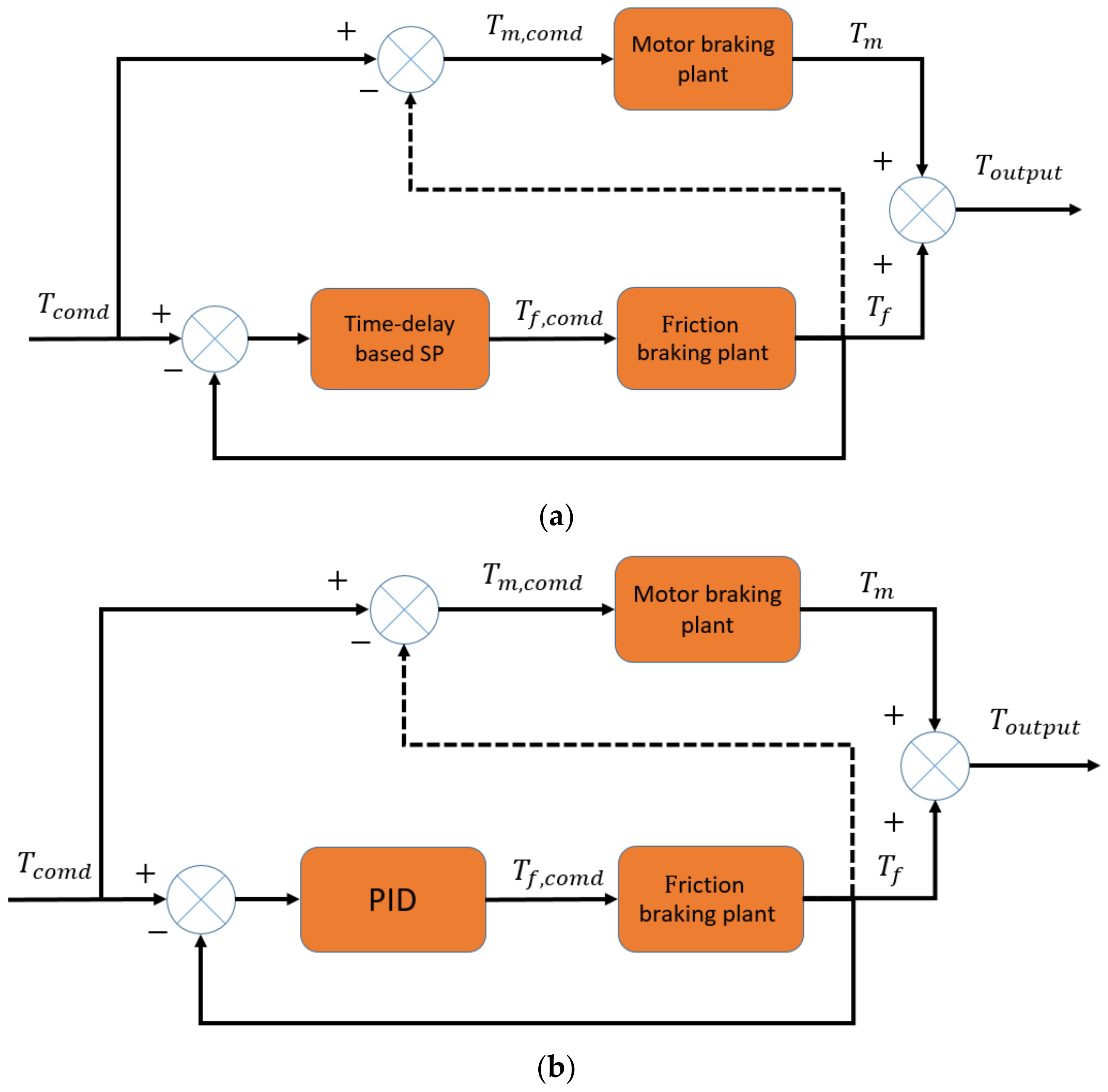
In the second set of simulation tests, the input time-delay-based Smith Predictor controller was tested, and PID control was adopted for comparison. For this test, the input time-delay is set to $0.2 s$, and other braking system parameters are shown in Table 1. The control structures are shown in Figure 9a,b. The difference between these two structures is the controller. The input time-delay-based Smith Predictor controller is shown in Figure 9a. In this test, it is assumed that the input time-delay of the friction braking system is known and is directly used in the input time-delay-based Smith Predictor controller. The PID controller is shown in Figure 9b. Since the response speed of motor braking is fast and the motor usually has a proprietary controller, the motor control is not taken into consideration. In this paper, the maximum braking torque of motor braking is set to $100 Nm$.

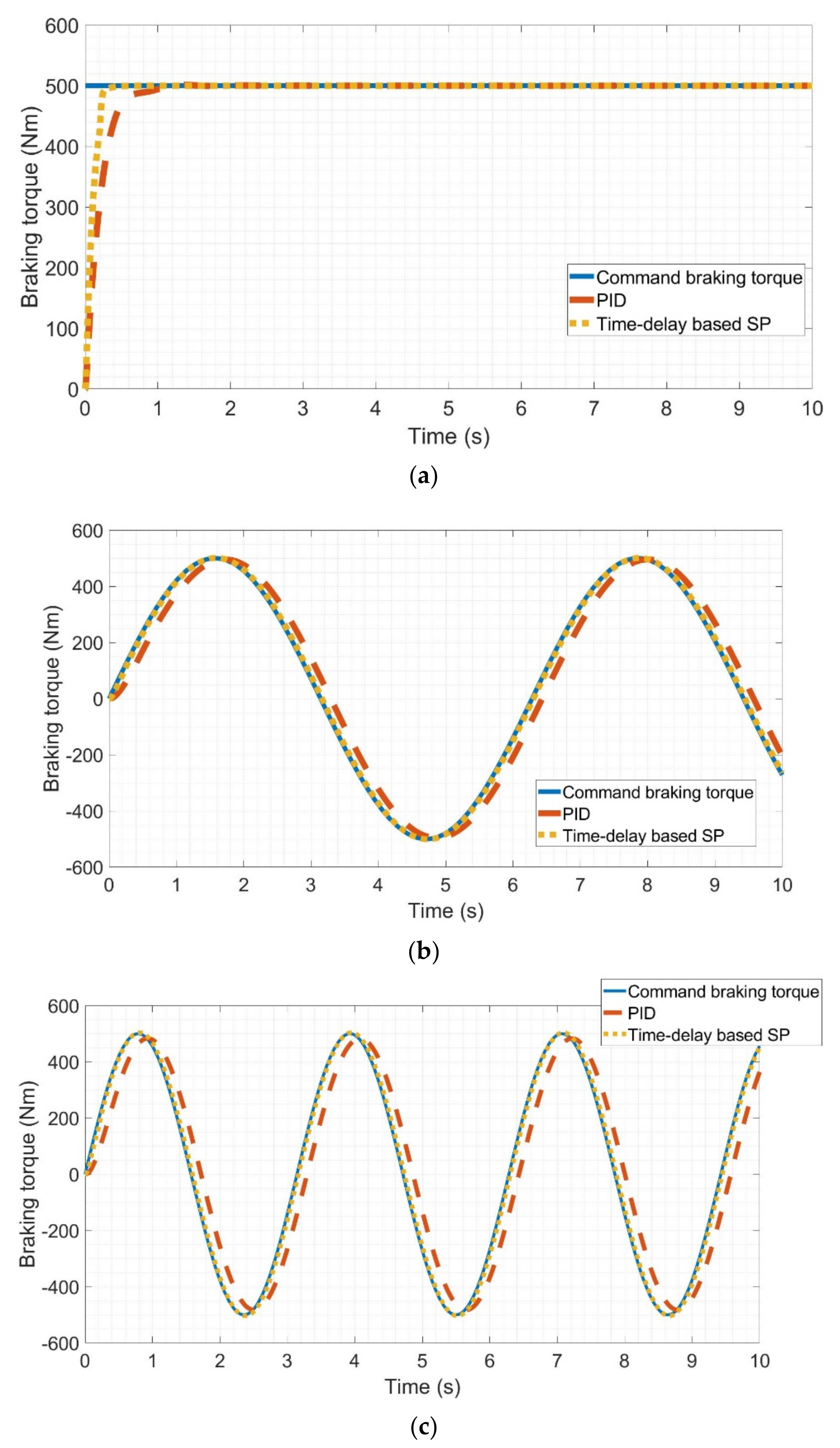
In order to compare the tracking performance of the two control algorithms in the blended braking system, two kinds of signals are used as the command signal. As shown in Figure 10a–c, the step signal and sinusoidal signals are set as the command signals. The step signal and sinusoidal signal are used to simulate emergency braking and normal braking, respectively. The step signal is used to simulate the rapid depression of the brake pedal, and the sinusoidal signal is used to simulate the process of slowly stepping on and raising the brake pedal. The step command is set to $500 Nm$. Sinusoidal command signals are set with an amplitude of $500 Nm$ and a frequency of $1 rad/s$, $500 Nm$ and a frequency of $2 rad/s$. The simulation results are shown in Figure 10a–c.

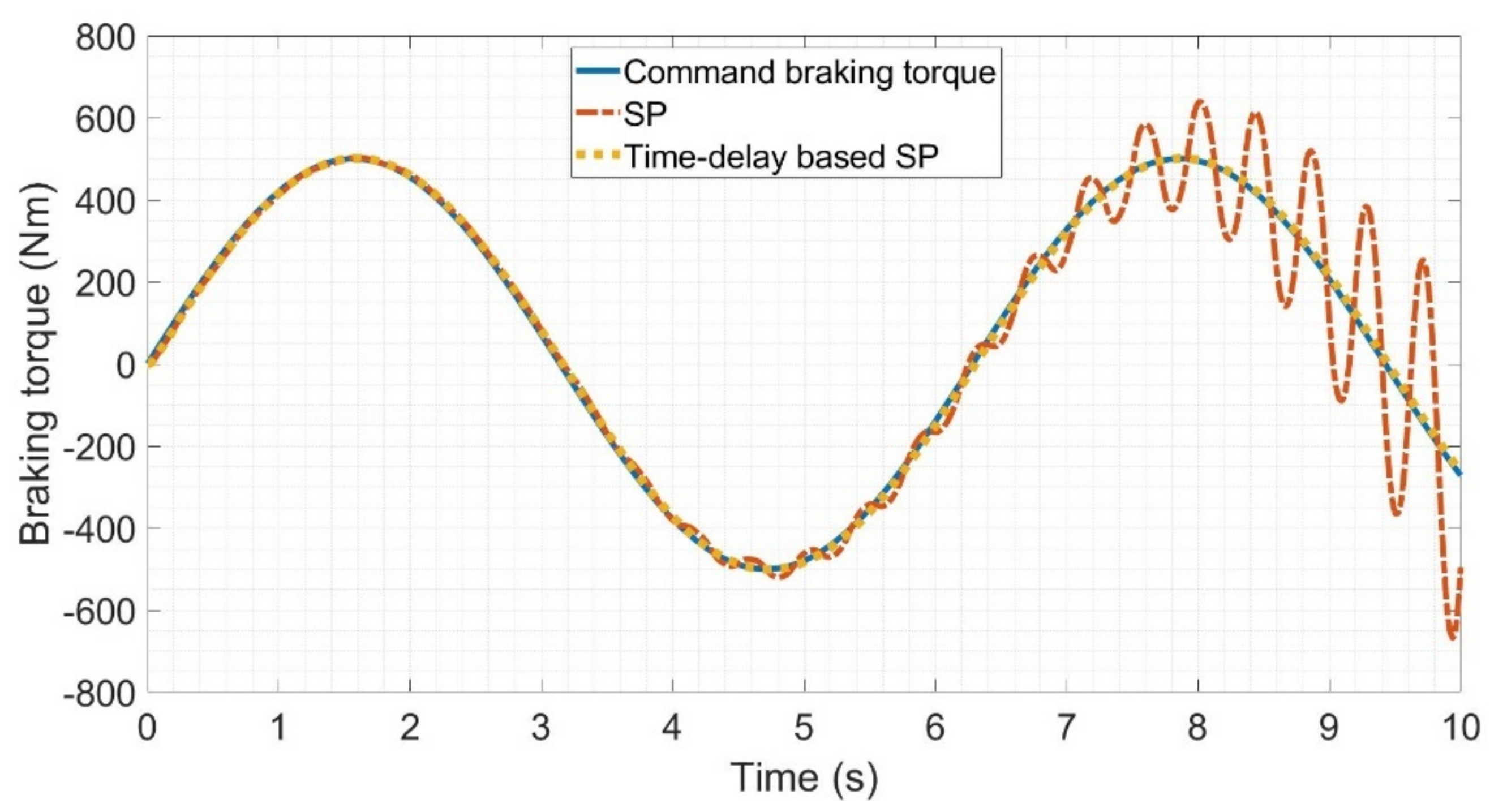
It can be seen from Figure 10a,b that the input time-delay-based SP can effectively track the command braking torque, regardless of the value of the command braking torque. Compared with the PID control for the blended braking system, the input time-delay-based SP has a faster response (as shown in Figure 10a). As shown in Figure 10b, the output signal under PID control cannot effectively track the command signal. This is due to the fact that the friction braking system under PID control has a slow response. As a result, the output braking torque of the friction braking system cannot effectively track the command braking torque. As the command braking torque increases, the difference between the command braking torque and the output braking torque increases. When this difference is larger than the maximum braking torque of the motor, the output braking torque of the motor cannot compensate for the difference between the command braking torque and the output braking torque of the friction braking torque. As a result, when the command braking torque is large, it cannot be tracked by the output braking torque of the blended braking system (as shown in Figure 10b). In contrast to the blended braking system under PID control, the blended braking system under time-delay-based SP control is able to effectively track the command braking torque. This is due to the fact that the friction braking system under the time-delay-based SP control has a faster response. This decreases the difference between the command braking torque and the friction braking system’s output braking torque. In this situation, the braking torque provided by the motor is sufficient to compensate for this difference. Thus, the blended braking system is able to effectively track the command braking system. It can also be seen from Figure 10c that the proposed control method maintains good tracking performance at a higher frequency.

In order to prove the necessity of obtaining an accurate estimation of the input time-delay, two groups of simulations were performed. In this test, the sinusoidal signal command signal has an amplitude of $500$ and a frequency of $1 rad/s$. The simulation model is the same as that in Figure 9. The input time-delay is $0.2 s$ for both the model and time-delay-based SP control. The input time-delay of SP control is $0.1 s$. The simulation results are shown in Figure 11.

As shown in Figure 11, the time-delay-based SP is able to effectively track the command braking torque when the input time-delay of the controller is the same as that of the model. It can also be seen that the system becomes unstable when the input time-delay of the controller is different from that of the model. This proves that the accurate estimation of the input time-delay is important for the time-delay-based SP control. For the friction braking system, the distance between the brake disc and the actuator changes with the braking system’s usage time and is hard to measure. Thus, the observer is necessary in this situation. This proves that the designed observer described in this paper is highly relevant.

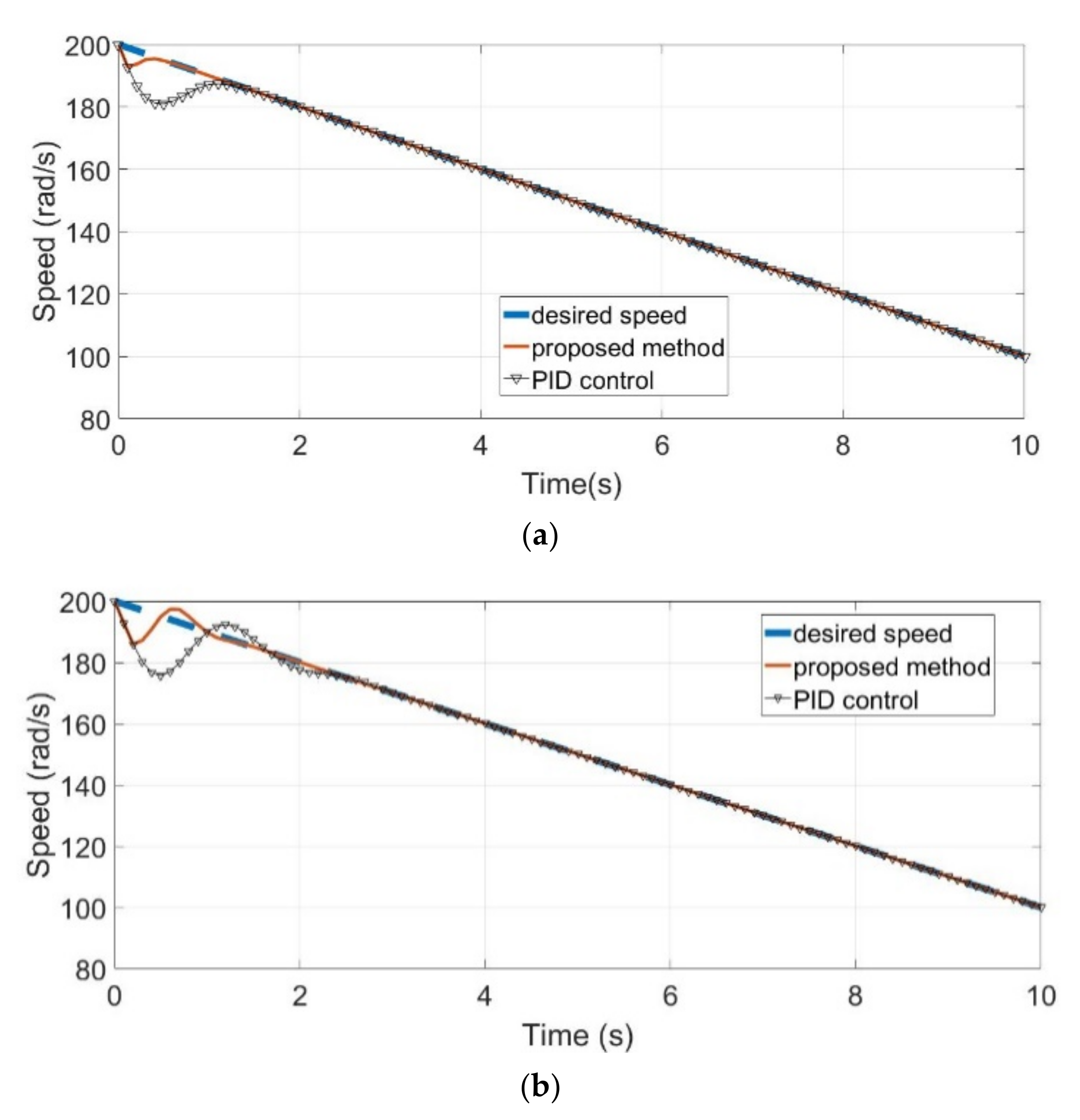
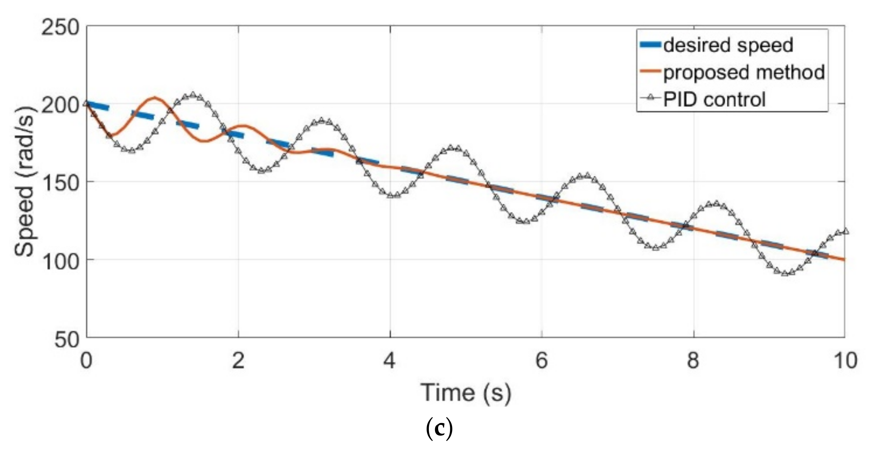
Finally, the proposed braking control method for the blended braking system (the control structure is shown in Figure 4) was tested in the case of normal braking.

In order to further verify the effectiveness of the proposed braking control method for the blended braking system (the control structure is shown in Figure 4), it was tested in a case of normal braking. In this test, vehicle braking during normal braking was tested. The initial wheel speed is $200 rad/s$, the input time-delay of the friction braking system is set to $0.1s$, $0.2 s$ or $0.3 s$ (in separate simulations), and the desired deceleration speed of the wheel is set to $10 rad/s^2$. The other relevant control parameters are listed in Table 1. For comparison, PID control is used to replace the time-delay-based SP control as the conventional blended braking systems’ controller (the control structure is shown in Figure 12). The simulation results are shown in Figure 13. Figure 13a–c shows the simulation results for time delays of $0.1$, $0.2,$ and $0.3 s$, respectively.

The controller’s parameters are adjusted when the time delay is 0.1 s. The relevant control parameters are adjusted so that the performance of the two controllers is as close as possible. As shown in Figure 13a, with both control methods, the vehicle wheel is able to effectively track the desired speed. When the adjusted control parameters remain unchanged and the input time-delay of the conventional blended braking systems is set to 0.2 s or 0.3 s, the vehicle is still able to effectively track the command signal with the proposed method (as shown in Figure 13b,c). However, under PID control, the braking command tracking performance becomes worse with the increasing input time-delay of conventional blended braking systems (as shown in Figure 13b,c). This proves that the proposed method has better tracking performance than the conventional PID control.

As shown in Figure 13, the proposed method has better tracking performance than the PID control. During the initial stage, there is a tracking error and chattering for the proposed method. This is due to the fact that the observer estimation error exists and the sign function exists in sliding mode control at the initial stage. When the observer obtains the accurate input time-delay and the tracking error of the wheel speed to the desired wheel speed becomes smaller, the proposed method is able to effectively track the command signal (as shown in Figure 13 after about $2 s$). However, the PID control consistently has a lower tracking performance. All of these simulation results prove that the proposed braking control method for the blended braking system is effective and important.

5. Discussion and Conclusions

In this study, an observer for a blended braking system comprising a motor braking system and friction braking system was designed. The simulation results prove that the designed observer is able to effectively estimate the input time-delay and the output braking torque of the friction braking system simultaneously. In addition, the sliding mode control is used to ensure that the wheel tracks the command wheel speed. The input time-delay-based Smith Predictor is adopted for the friction braking system control. The simulation results show that the input time-delay-based Smith Predictor has better tracking performance than the conventional PID control. In addition, the input time-delay parameter provided by the observer helps the Smith Predictor overcome the problem of an unknown input time-delay. The simulation results also show that the proposed control structure for the blended braking system has better braking performance than the traditional braking control method.

In the future, the braking torque distribution between the motor braking system and the friction braking system will be addressed. By coordinating the braking torque ratio between these two braking systems, the brake system can not only meet the braking requirements but also maximize the recovery of braking energy.