Design and Characterization of an Electrostatic Constant-Force Actuator Based on a Non-Linear Spring System

Abstract

In recent years, tissue engineering with mechanical stimulation has received considerable attention. In order to manipulate tissue samples, there is a need for electromechanical devices, such as constant-force actuators, with integrated deflection measurement. In this paper, we present an electrostatic constant-force actuator allowing the generation of a constant force and a simultaneous displacement measurement intended for tissue characterization. The system combines a comb drive structure and a constant-force spring system. A theoretical overview of both subsystems, as well as actual measurements of a demonstrator system, are provided. Based on the silicon-on-insulator technology, the fabrication process of a moveable system with an extending measurement tip is shown. Additionally, we compare measurement results with simulations. Our demonstrator reaches a constant-force of 79 ± 2 $\mathsf{\mu }$N at an operating voltage of 25 V over a displacement range of approximately 40 $\mathsf{\mu }$m, and the possibility of adjusting the constant-force by changing the voltage is demonstrated.

1. Introduction

This paper introduces an electrostatic constant-force actuator for an application in the analysis of viscoelastic materials [1] or the mechanical stimulation in tissue engineering [2]. This moveable microsystem is fabricated on a silicon-on-insulator (SOI) substrate and consists of an electrostatic comb drive and a non-linear spring system. A non-linear spring system generates a constant restoring force, which enables a constant-force reaction along a specific displacement. Recent research of restoring forces on microstructures, such as Timoshenko curved nanobeams or nonlocal gradient elastic beams, can be found in References [3,4,5]. Additionally, the comb drive generates also a constant voltage-controlled actuation force. Due to the linear dependency between the capacitance and the displacement, the actuator position can be measured in real-time.

Yang et al. [6] establish a passive-type constant-force microgripper. In their system, the constant force is realized using a combination of inclined bi-stable beams and straight leaf flexures. The microgripper is designed using two separate parts of actuation and constant force modules. The actuation part is driven by six pairs of electrothermal Z-shaped beams that offer a large displacement at low voltage. The resulting constant force is achieved by a combination of positive- and negative-stiffness mechanisms. Zhang et al. [7] propose a similar design in a macroscopic actuation system. Nevertheless, the actuation force is generated with an external linear actuator. Previous research tends to focus on the constant-force actuation rather than the integrated simultaneous measurement of the actual system displacement, as established in the system presented in this work.

The arrangement of the electrostatic comb drives of the presented constant-force actuator is used to enable the constant actuation force on a large travel range, which is introduced by Legtenberg et al. [8]. Comb drives allow for a simultaneous constant force actuation and capacitance measurement. In this paper, the measurement of the capacitance is used to calculate the actual position of the constant-force actuator.

This work focuses on the design and characterization of a new constant-force actuator. The first section of this paper examines the analytical description of the comb drive and the non-linear spring system. Then, a numerical simulation results in the constant-force chip design.

Noteworthy is the extending and moveable measurement tip, that is necessary to reach a sample with the constant-force system. The free tip is fabricated on the silicon-on-insulator using a dicing free process [9] and a predetermined breaking point [10]. Finally, the experimental setup is described, and the characterization of the different components on the microchip is discussed.

2. Materials and Methods

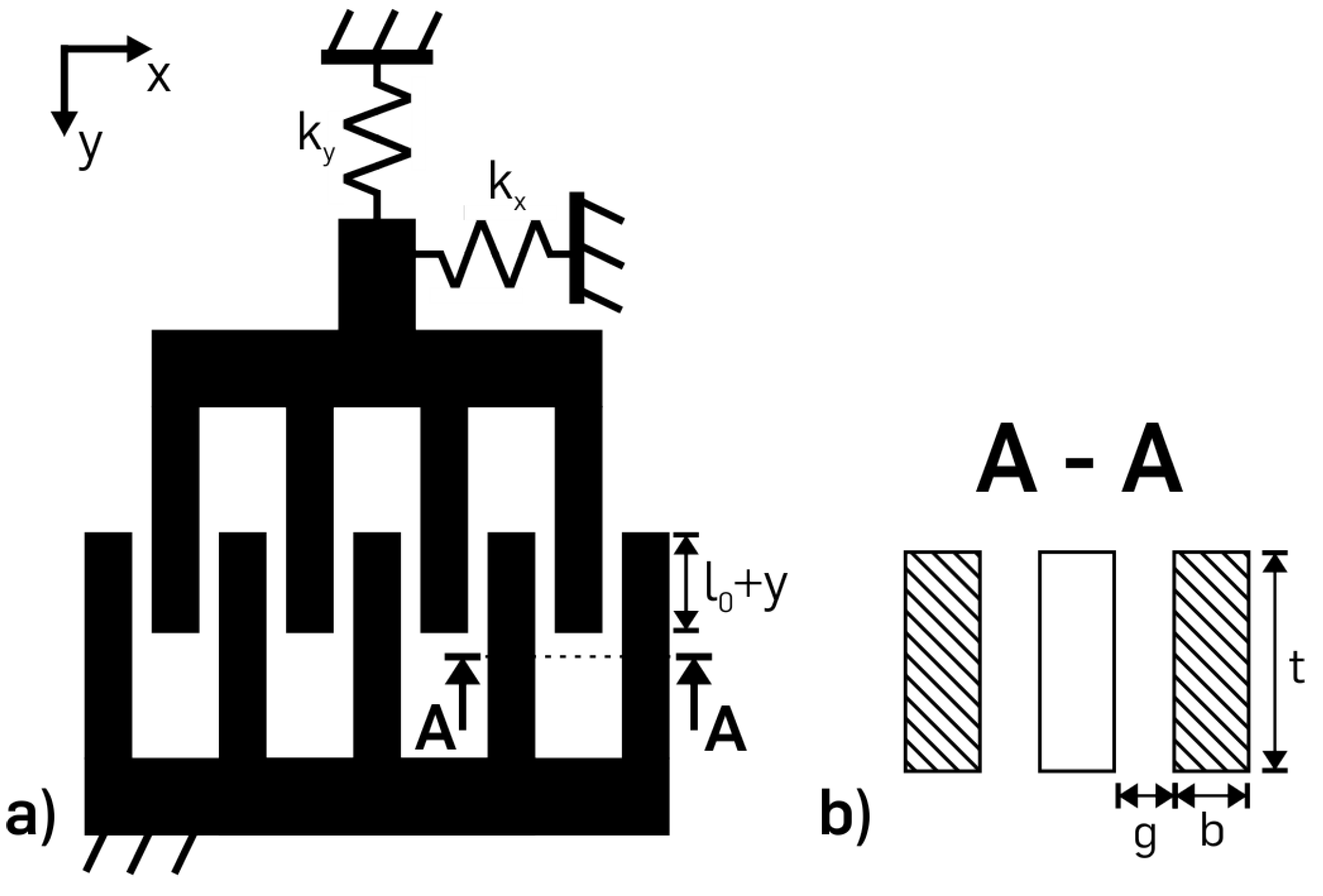
2.1. Electrostatic Comb Drive Actuator

As Figure 1 demonstrates, the actuator consists of two electrically conductive combs. One comb is mechanically fixed while the other is suspended on an elastic suspension spring. Detailed analytical descriptions of comb drives can be found in References [8,11]. The design of the suspension spring is essential in order to eliminate unwarranted angular motion of the rotor [12]. It is designed to have a low stiffness $k_{\mathrm{y}}$ parallel to the comb fingers and a much higher stiffness $k_{\mathrm{x}}$ in the transverse direction. The formula for the capacitance of the comb drive is given by

$$C=\frac{2n{\mathsf{ϵ}}_0{\mathsf{ϵ}}_{\mathrm{r}}t}{g}(l_0+y),$$

(1)

where n is the number of the fingers of the movable comb, ${\mathsf{ϵ}}_0$ is the dielectric constant, ${\mathsf{ϵ}}_{\mathrm{r}}$ is the relative permittivity, t is the depth of the fingers, g is the gap spacing between the fingers, and $A=t(l_0+y)$ is the overlapping area with $l_0$ as the initial comb finger overlap and y as the displacement in y-direction.

Equation (1) indicates that the capacitance is linear to the comb drive displacement in y-direction. The differential measurement method $\Delta C=|C_1-C_2|$, where the capacitance $C_1$ increases and $C_2$ decreases during the system displacement in y-direction, is commonly used to reduce the influence of temperature and environmental changes over time.

In case of voltage control, the lateral electrostatic force for the comb drive in the y-direction $F_{\mathrm{el},\mathrm{y}}$ can be calculated by

$$F_{\mathrm{el},\mathrm{y}}=-\frac{\mathrm{d}{W}_{\mathrm{el}}}{\mathrm{d}y}=-\frac{n{\mathsf{ϵ}}_0{\mathsf{ϵ}}_{\mathrm{r}}t}{g}·U^2,$$

(2)

with U as the applied voltage. From this calculation, it is clear that the electrostatic comb drive force is independent of y and the finger overlap $l_0$. Because of that, the electrostatic comb drive actuator can generate a constant force that is proportional to $U^2$.

Ideally, the vertical electrostatic force for comb drive actuators in the x-direction $F_{\mathrm{el},\mathrm{x}}=F_{\mathrm{el},{\mathrm{x}}^{+}}-F_{\mathrm{el},{\mathrm{x}}^{-}}$ is almost zero with

$$F_{\mathrm{el},{\mathrm{x}}^{+}}=F_{\mathrm{el},{\mathrm{x}}^{-}}=\frac{n{\mathsf{ϵ}}_0{\mathsf{ϵ}}_{\mathrm{r}}t(l_0+y)}{2{(g\pm x)}^2}{U}^2.$$

(3)

However, this ideal theoretical situation does not translate into reality, and large suspension springs are required to suppress the corresponding forces within the mechanical structure. Especially in comb drive actuators, the vertical force causes side instability as a limiting condition. Above a certain voltage, the comb drive operates as a parallel-plate actuator perpendicular to the common movement direction. This unwanted effect requires a careful optimization of the actuator and the mechanical spring for a large displacement [13].

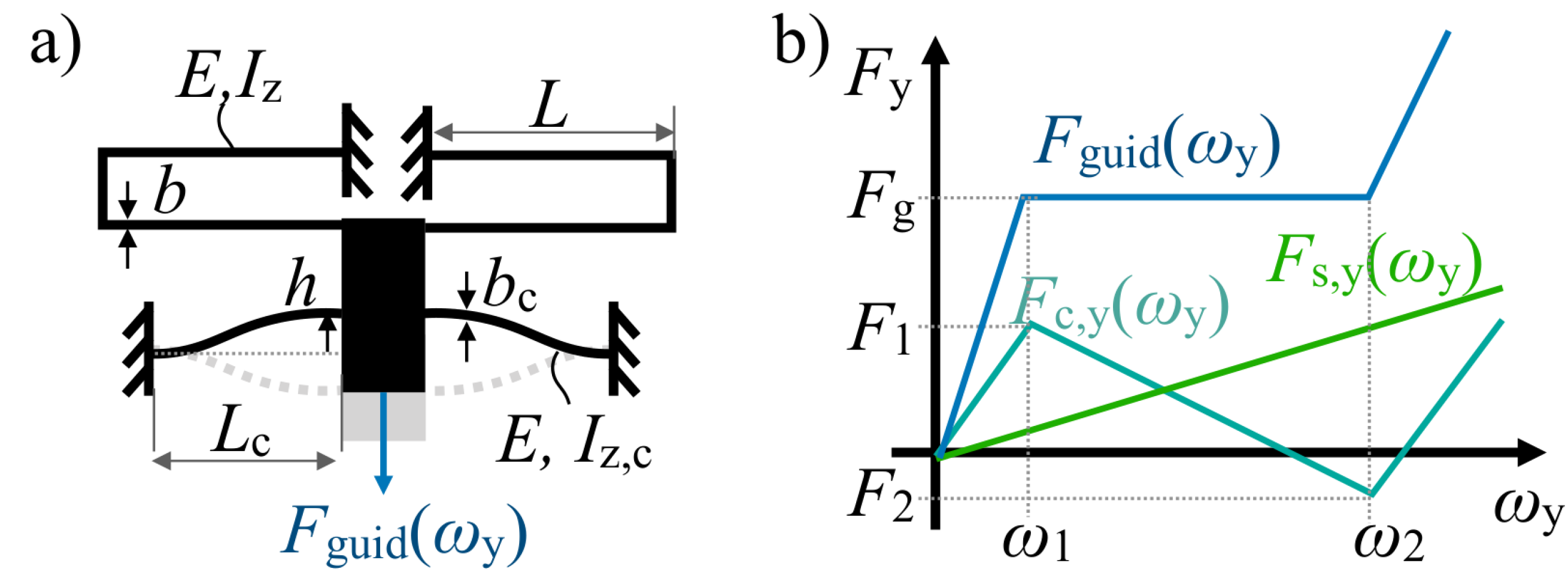
2.2. Non-Linear Spring System

Although the electrostatic actuator generates a constant force, which is independent of the position, the actuator still requires guiding springs, allowing a translational displacement. Serpentine springs [8,14] are commonly used. Considering the ratio of the spring rate in axial and off-axial direction, triangular springs [15] are also well suited. However, by implementing linear springs, the constant force characteristic of the actuator system can be affected, since the restoring force is usually an almost linear function of displacement. For a constant-force system, the force-displacement characteristic of the guiding springs should be constant, as well. A constant force-displacement characteristic can be tailored by combining a mechanical anti-spring featuring a negative spring rate with a linear spring, as indicated in Figure 2.

Since the restoring force of the combined spring system is the superposition of both springs, the negative and positive spring rate compensate each other, resulting in a constant and position-independent force reaction. Considering a serpentine spring as shown in Figure 2 and regarding small displacements in relation to spring size, the restoring force of the spring is known to be:

$$F_{\mathrm{s},\mathrm{y}}\left({\omega }_{\mathrm{y}}\right)=k_{\mathrm{s},\mathrm{y}}{\omega }_{\mathrm{y}}=\frac{12E{I}_{\mathrm{z}}}{L^3}{\omega }_{\mathrm{y}}$$

(4)

The expression is based on Euler-Bernoulli beam theory, which also shows high validity for beams realized in monocrystalline silicon. For the design of an anti-spring, a cosine-shaped beam is used, which is described by:

$$\omega \left(x\right)=\frac{h}{2}\left(1-\cos \left(\frac{2\pi x}{L_{\mathrm{c}}}\right)\right).$$

(5)

The force-displacement characteristic of the mechanical anti-spring can be calculated by buckling beam analysis. For curved beams, which fulfill the condition of $h/b\ge 6$, Qiu et al. [16] propose an approximation for the calculation of the characteristic positions ${\omega }_1,{\omega }_2$ and $F_1,F_2$ of the force-displacement characteristic. Based on these approximations, the force can be written as follows:

$$F_{\mathrm{c},\mathrm{y}}\left({\omega }_{\mathrm{y}}\right)\approx \{\begin{array}{cc}578.1\frac{E{I}_{\mathrm{c},\mathrm{z}}}{L_{\mathrm{c}}^3}{\omega }_{\mathrm{y}}\hfill & 0<{\omega }_{\mathrm{y}}<0.16h\\ \frac{E{I}_{\mathrm{c},\mathrm{z}}}{L_{\mathrm{c}}^3}(\frac{185}{2}h-78.84{\omega }_{\mathrm{y}})\hfill & 0.16h\le {\omega }_{\mathrm{y}}<1.92h\end{array}.$$

(6)

The force-displacement characteristic of the combined spring system finally results in:

$$F_{\mathrm{guid},\mathrm{y}}\left({\omega }_{\mathrm{y}}\right)\approx \{\begin{array}{cc}\left(\frac{12E{I}_{\mathrm{z}}}{L^3}+578.1\frac{E{I}_{\mathrm{c},\mathrm{z}}}{L_{\mathrm{c}}^3}\right){\omega }_{\mathrm{y}}\hfill & 0<{\omega }_{\mathrm{y}}<0.16h\\ \left(1+\frac{12E{I}_{\mathrm{z}}}{L^3}\right)\left(\frac{185}{2}\frac{E{I}_{\mathrm{c},\mathrm{z}}}{L_{\mathrm{c}}^3}h-78.84\frac{E{I}_{\mathrm{c},\mathrm{z}}}{8L_{\mathrm{c}}^3}{\omega }_{\mathrm{y}}\right)\hfill & 0.16h\le {\omega }_{\mathrm{y}}<1.92h\end{array}.$$

(7)

The width of both segments in the force-displacement characteristic can only be controlled through the design of the initial deflection of the curved beam. Additionally, a compensation of the positive and negative spring rate is valid for displacements $0.16h\le {\omega }_{\mathrm{y}}$. For an ideal compensation, the constant restoring force yields:

$$F_{\mathrm{g}}=0.16hE\left(\frac{12I_{\mathrm{z}}}{L^3}+578.1\frac{I_{\mathrm{c},\mathrm{z}}}{L_{\mathrm{c}}^3}\right).$$

(8)

The force-displacement characteristic is simulated by FEM simulations carried out in COMSOL Multiphysics. A 2D geometry of the non-linear spring system is used for this linear elastic simulation (see Figure 3).

In the solid mechanics interface, the depth of the 2D component is set to 20 $\mathsf{\mu }$m. The six rounded shoulder fillets are tied to fixed constraints, and a prescribed displacement parameter in y-direction is set. The fine mesh comprises a minimal element size of 0.5 $\mathsf{\mu }$m, which is more than sufficient for the simulation. In the stationary study, the prescribed displacement parameter varies from 0 to 70 $\mathsf{\mu }$m by the step size of 1 $\mathsf{\mu }$m. Taking non-linearities in consideration, the reaction force in y-direction can be simulated. Figure 3 shows the simulation results of a spring system compared to the theoretical results. Both models are performed on the basis of the Young’s modulus in [110] direction of monocrystalline silicon and the Poisson’s ratio is neglected for simplicity. The chart shows that there are differences between the numerical and analytical constant-force of approximately $10\%$. This factor may partly be explained by the rounded shoulder fillets of the simulated non-linear spring system to protect the beams from breaking at the clamping. However, the final design of the springs is manually optimized by varying the parameters of the component geometry. In further work, the Nelder-Mead algorithm or the multilevel coordinate search [17] can be used for systematic non-linear optimization.

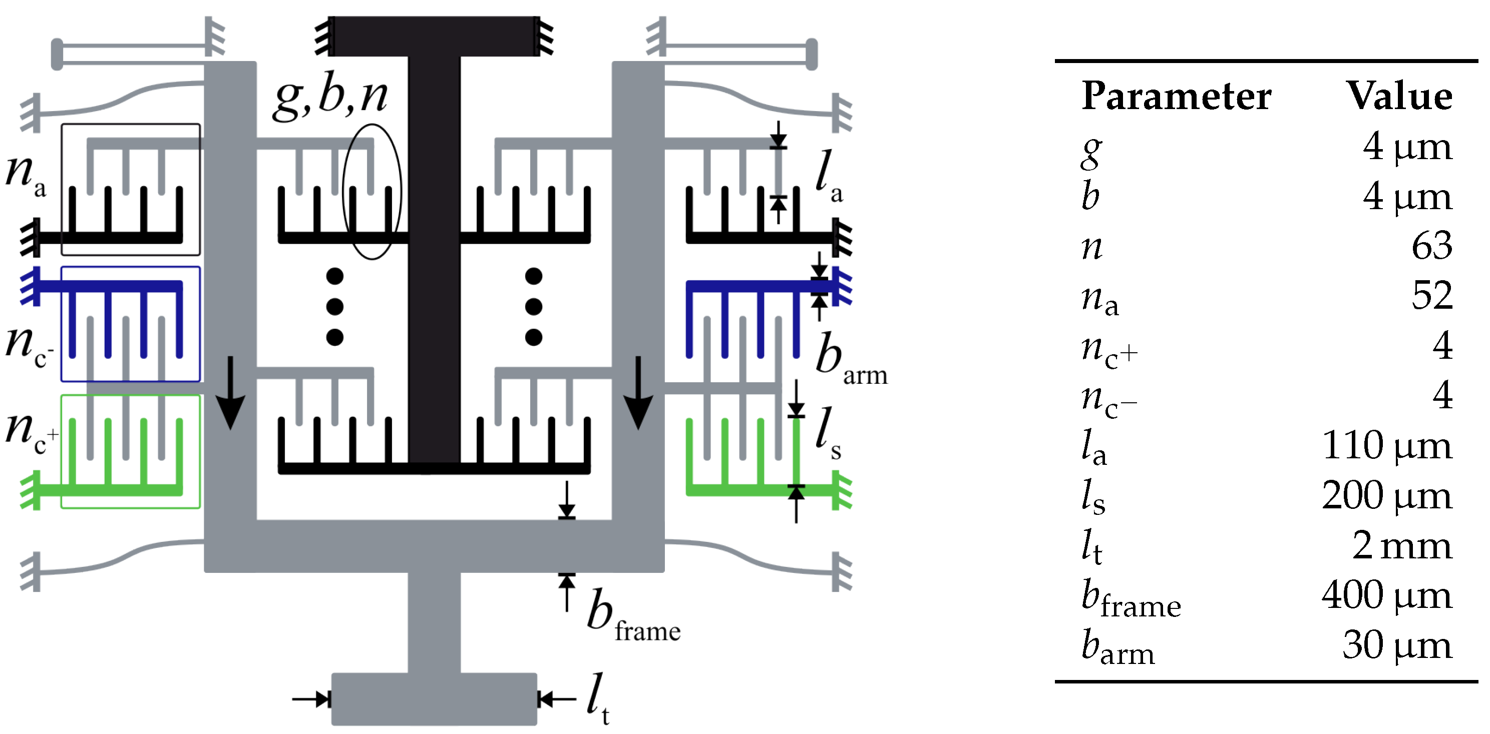
2.3. Design of the Constant-Force Generator

The proposed constant-force microchip combines an electrostatic actuation and a non-linear spring system (Figure 4). For the electrostatic force generation, the actuator consists of $n_{\mathrm{a}}=52$ moving combs featuring $n=62$ fingers each. For the differential capacitance measurement method, there are four differential capacitors on each side of the frame. The gap between the finger electrodes, as well as the width of the fingers themselves, is 4 $\mathsf{\mu }$m. A mechanical barrier stops any undue displacements of the system as a precaution against overextension of the springs. A patterned honeycomb structure of the moveable parts reduces the mass load by approximately $80\%$. Therefore, the weight force of $F_{\mathrm{m}}\approx 0.58$ $\mathsf{\mu }$N is negligible. For this reason, the constant-force $F_{\mathrm{y}}$ results only from the electrostatic force $F_{\mathrm{el}},\mathrm{y}$ and the non-linear spring system force $F_{\mathrm{guid}}$:

$$F_{\mathrm{y}}=F_{\mathrm{el}},\mathrm{y}-F_{\mathrm{guid}}.$$

(9)

Therefore, the non-linear spring force needs to be surpassed by the electrostatic actuation ($F_{\mathrm{el}},\mathrm{y}>F_{\mathrm{guid}}$) to move the measurement tip. The dimensions of a single chip design are 6.5 × 7.5 ${\mathrm{mm}}^2$, and the measurement tip has a length of $l_{\mathrm{t}}=2$ mm. This dimension can be adapted individually for every application by slightly changing the mask design.

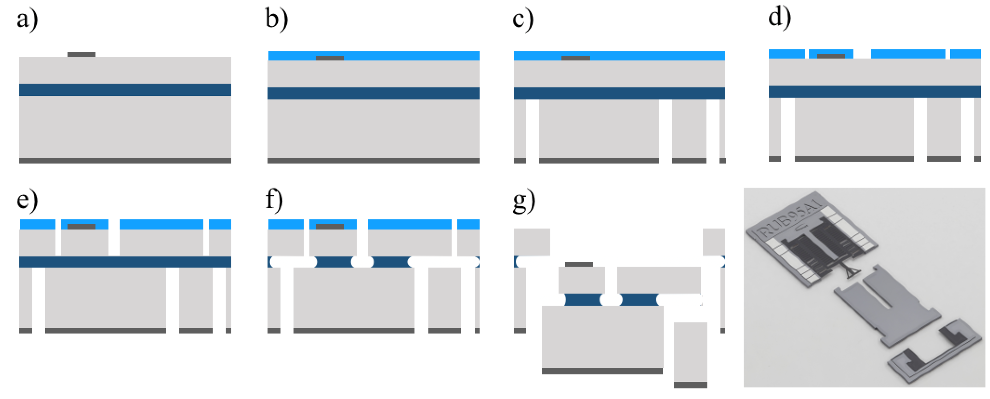
2.4. Fabrication Process

The demonstrators are fabricated using a SOI-based dicing free process known from, e.g., References [9,18]. The main processing steps are shown in Figure 5. A (100)-oriented SOI substrate with 20 $\mathsf{\mu }$m thick device layer and handle layer of 400 $\mathsf{\mu }$m thickness is used. First, a 100 nm thick aluminium layer is deposited on the handle and device layer by evaporation. On the device layer, the aluminium serves as electrode material and is patterned by wet chemical etching (a). In a second step, a ${\mathrm{SiO}}_2$ hard mask is deposited by PECVD (b). For the release of the chips from the substrate, the aluminium on the handle layer is patterned by wet etching and then etched using deep reactive ion etching (c). In a second deep etching step (e), the mechanical structures on the device layer are etched subsequently after the patterning of the ${\mathrm{SiO}}_2$ hard mask (d). Next, an HF-vapor process is used to release the mechanical structures by etching the ${\mathrm{SiO}}_2$ underneath the moveable structures (f). In this processing step, the chips, as well as the backside, are also released from the wafer without dicing (g). Finally, the protection structure for the measurement tip is severed at the predetermined breaking point.

2.5. Electronical Voltage Control

For the robust and reproducible deflection of the microsystem, an control circuit is developed based on a microcontroller. In addition to the provision of a minimum current amplitude, this circuit has to also provide a reliable and stable voltage supply. To achieve this, the pulse width modulation (PWM) feature of an Arduino Mega 2560 microcontroller is used in combination with a lowpass transistor circuit as shown in Figure 6.

The microcontroller provides an 8-Bit PWM resolution, which results in 256 output voltage values between 0 V and 5 V. This PWM output is then transferred to the base of a NPN transistor that switches a supply voltage $U_{\mathrm{dd}}$ between 0 V and 140 V (1). In its conducting state, triggered by a base-emitter voltage $U_{\mathrm{BE}}$ of 5 V, the supply voltage is attenuated by the voltage divider consisting of the resistors $R_3$ and $R_4$. A base-emitter voltage $U_{\mathrm{BE}}$ of 0 V leads to the isolation of the transistor and, thus, to a transfer of the entire supply voltage to the next circuit stage. After lowpass filtering, the resulting output voltage $U_{\mathrm{o}}$ (2) is given by

$$U_{\mathrm{o}}=U_{\mathrm{dd}}-U_{\mathrm{BE}}·\frac{R_3}{R_4}·\frac{n_{\mathrm{bit}}}{255},$$

(10)

where $n_{\mathrm{bit}}$ represents the bit value of the microcontroller.

Due to the difference of the spring constants in the x- and y-direction, an overlaid alternating voltage is needed to compensate the lateral displacement of the microactuator elements [19,20]. This voltage is generated by an additional transistor whose base is connected to the clock signal with a variable frequency between 144 Hz and 8 MHz (3). The high lowpass resistance leads to a very low collector current into this second transistor, which is in the range of 10 $\mathsf{\mu }$A to 50 $\mathsf{\mu }$A. Parasitic effects start to affect the collector-emitter voltage $u_{\mathrm{CE}}$ whose usual linear dependency to the base-emitter voltage $u_{\mathrm{BE}}$ is disrupted [21]. For a known collector-emitter capacitance $C_{\mathrm{CE}}$ in combination with the base-collector resistance $r_{\mathrm{BC}}$ and the base-collector capacitance $C_{\mathrm{BC}}$, the relation between those two voltages can be described by

$$\frac{u_{\mathrm{CE}}}{u_{\mathrm{BE}}}=\frac{1-{\left(\omega r_{\mathrm{BC}}{C}_{\mathrm{BC}}\right)}^2}{1+4\omega r_{\mathrm{BC}}{C}_{\mathrm{BC}}-{\left(\omega r_{\mathrm{BC}}{C}_{\mathrm{BC}}\right)}^2}·\frac{1}{\sqrt{1+\left(\omega C_{\mathrm{CE}}\right)}},$$

(11)

which corresponds to the product of the transfer functions of a band-stop-filter and a lowpass-filter at $\omega$ [22]. The resistances and capacities represent transistor parameters that cannot be modified by external wiring.

To ensure the reproducible deflection of the microsystem, it is necessary to charge the capacitor plates in a shorter time than one period of the systems cutoff frequency. This requires an electrical current amplification of the output signal (4) as the limited lowpass output current is unable to deliver a sufficiently large current to the electrodes in time. The current amplification is realized in a buffer amplifier circuit, that provides a maximum current of 1.4 mA, a sufficient amount to charge the capacitor electrodes within nanoseconds. An electromechanical relay provides the required steep voltage rise that leads to the abrupt force generation within the microsystem. In the Appendix A,

Table A1. Values and types of used electrical components.

Component	Value	Type
$R_1$	47 k$\Omega$	-
$R_2$	1 k$\Omega$	-
$R_3$	4.7 k$\Omega$	-
$R_4$	1 k$\Omega$	-
NPN transistor	-	ON 2N5551 160 V bipolar junction transistor
$R_{\mathrm{Lowpass}1}$	1 M$\Omega$	-
$C_{\mathrm{Lowpass}1}$	10 nF	-
$R_{\mathrm{Lowpass}2}$	1 M$\Omega$	-
$C_{\mathrm{Lowpass}2}$	10 nF	-
Relay	-	KY-019 5V magnetic relay
$R_6$	100 k$\Omega$	-
$R_7$	470 $\Omega$	-
$R_8$	1 M$\Omega$	-

displays the values and types of the electrical components used within the described circuit.

2.6. Experimental Setup for the Force Measurement

The completed microchip is glued onto a printed circuit board (PCB) with a carbon conductive paste for the electrical connection of the microsystem. The aluminium bondpads on the chip in Figure 7a were connected to the contacts on the PCB by bonding with aluminium wire. The handle layer and the moveable parts on the chip are connected to ground for the electric protection of the measured sample. The non-moveable electrostatic combs of the actuation comb drive ($C_{\mathrm{a}}$) are connected to the input voltage on the PCB. For the differential capacitance measurement, the four sensor pads $C_{\mathrm{s}1}$, $C_{\mathrm{s}2}$, $C_{\mathrm{s}3}$, and $C_{\mathrm{s}4}$ were connected separately onto the PCB. The PCB includes pin headers for the electrical connection to voltage control and the capacitive sensing chip on a separate board. This allows for an easy exchange of the constant-force actuators, since all actuators can be controlled with the same electronics.

The capacitance measurement is realized by the FDC1004Q capacitance-to-digital converter of Texas Instruments. This sensing chip has a measurement resolution of 0.5 fF for an input range of ±15 pF [23]. Its ${\mathsf{I}}^2$C interface allows the programmable connection with the Arduino Mega 2560 microcontroller. The power supply for the FDC1004Q of 3.3 V is also provided by the microcontroller. The FDC1004Q can measure the capacitance between the channel inputs and ground. With its functional mode for differential measurement by

$$\Delta C_1=C_{\mathrm{s}1}-C_{\mathrm{s}3}$$

(12)

and

$$\Delta C_2=C_{\mathrm{s}2}-C_{\mathrm{s}4},$$

(13)

the returned data is almost independent of environmental influences. For the FDC1004Q, it is necessary that the capacities $C_{\mathrm{s}1},C_{\mathrm{s}2}$ increase and $C_{\mathrm{s}3},C_{\mathrm{s}4}$ decrease while the system is moving in y-direction. At all times, these assertions should be fulfilled: $C_{\mathrm{s}1}>C_{\mathrm{s}3}\mathrm{and}{C}_{\mathrm{s}2}>C_{\mathrm{s}4}$. For best results, the sensing-chip is located as close as possible to the capacitive sensors. Constant parasitic capacities of the PCB connection can be regarded as a constant capacitive offset.

The experimental setup for force measurement makes use of a high precision balance (Sartorius WZA 224-N) and a piezo linear stage (PI Q-545). The control of these components is realized in a LabVIEW program that calculates the force from the measured weight with $F=m·g$ and $g=9.81{\mathrm{m}/\mathrm{s}}^2$. The standard deviation of the balance is given by $\pm 0.1$ mg, which equals approximately 1 $\mathsf{\mu }$N, and the minimum time to stabilize the measurement is 0.6 s [24]. The time between two measurements is set to 1.5 s. The piezo linear stage has a maximal displacement of 13 mm, a minimal increment of 6 nm and a resolution of 1 nm with a repeatability of 100 nm [25]. As described in Figure 7b, the microchip is fixed to the linear stage that can displace the system in y-direction, positioned vertically to the balance measurement surface. The correct alignment can be controlled optically by a microscope.

This setup allows for two different experimental methods: the first method comprises the force measurement of the non-linear spring system without electrical actuation. A needle on the balance is attached to the moveable structure of the chip. When the linear stage moves the PCB upwards step by step, the mass of the needle on the balance is getting lower and the force of the spring system can be measured. The second method is used for the constant-force measurement with electrical actuation. In this case, the needle is directly placed under the measurement tip. Then, the power supply for the comb drive actuation is activated and the resulting constant-force can be measured at the balance. When the stage ascends, the measurement tip exerts pressure on the needle and the resulting force can be measured until the contact to the needle is lost. Simultaneously to the actuation, the deflection can be measured using the capacitance and the sensing-chip.

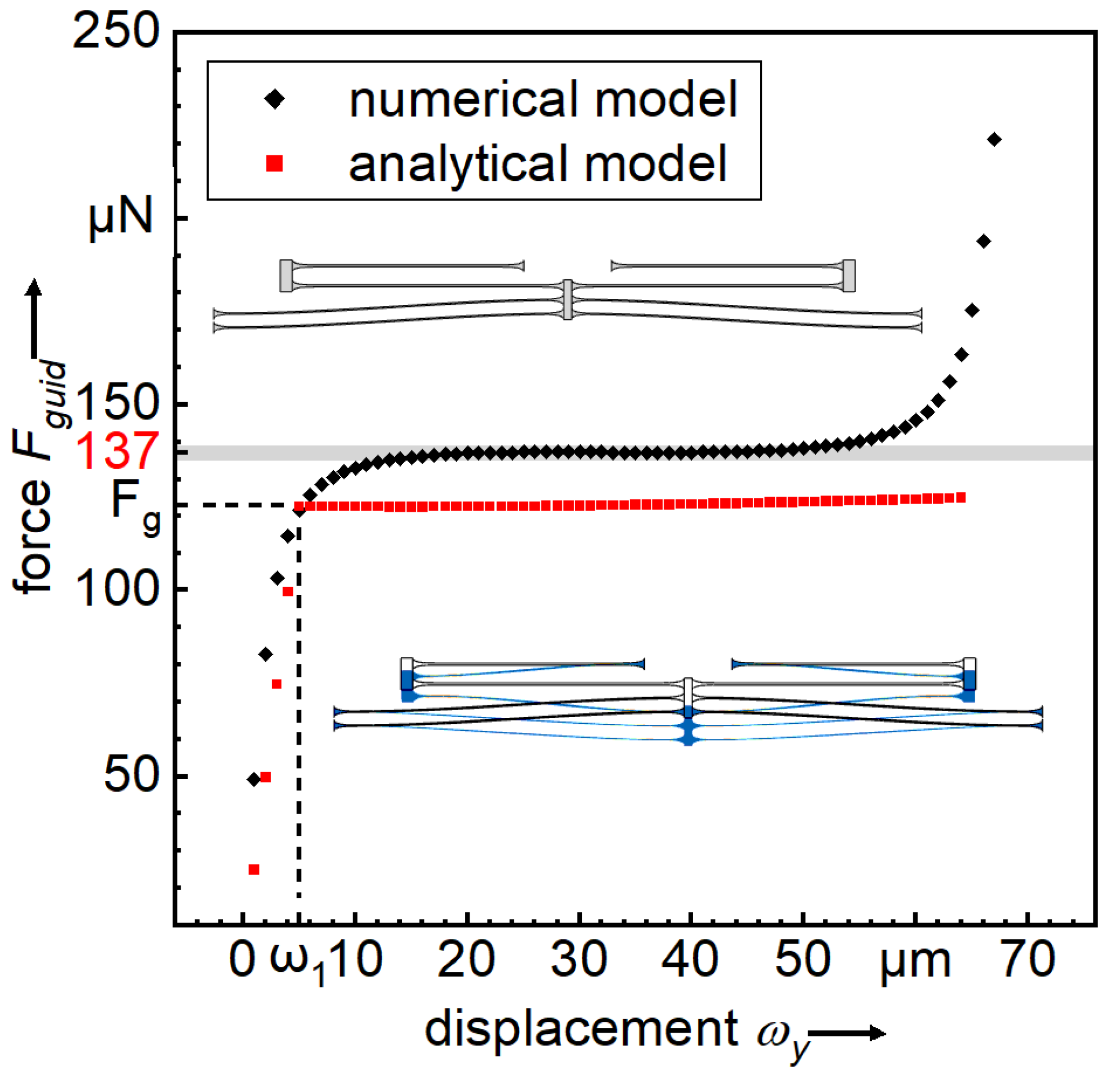
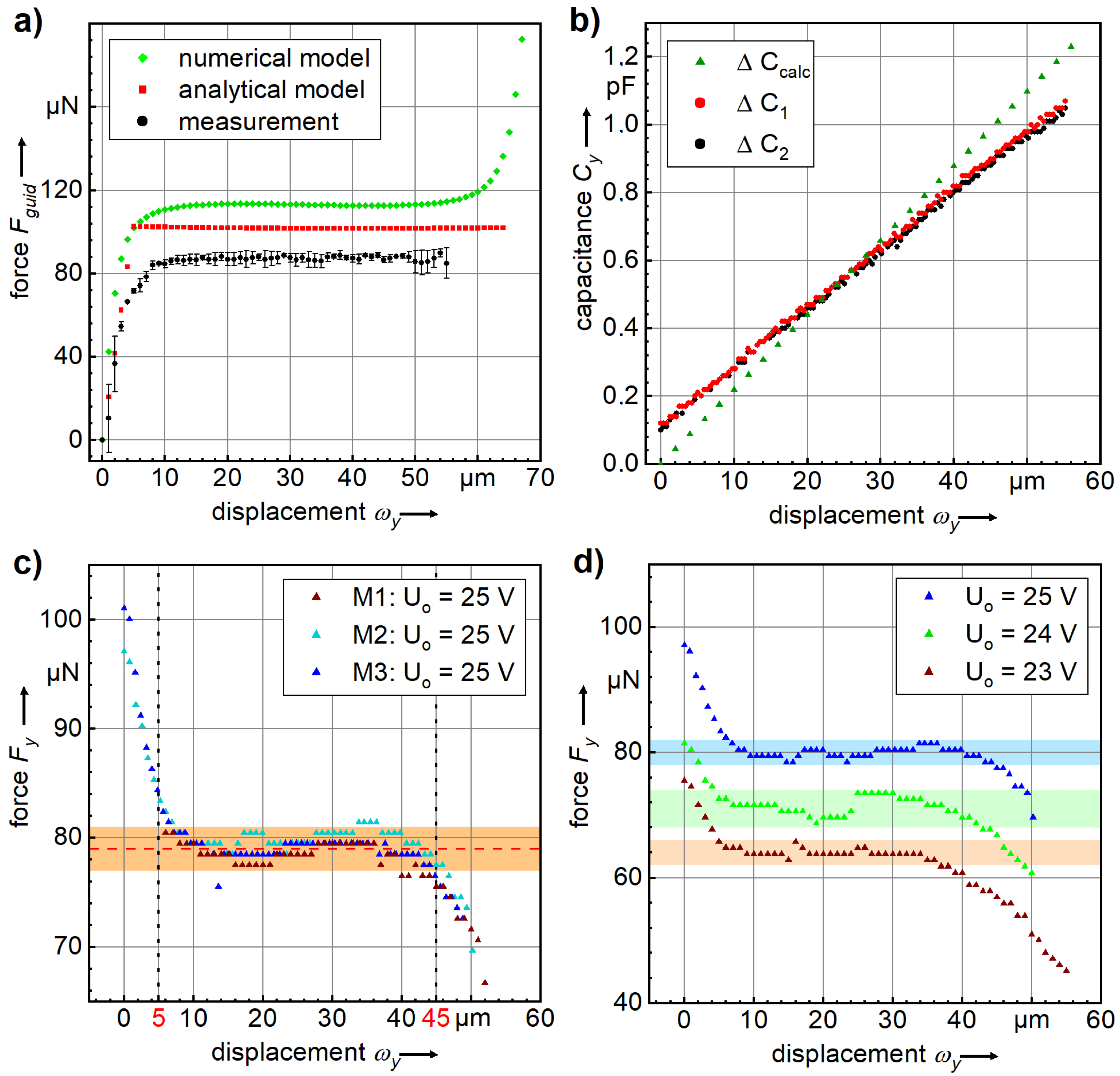
3. Experiments and Characterization

The constant-force characteristic of the non-linear spring system is shown in Figure 8a (black dots). This measurement graph depicts the average of three force measurements and the standard deviation. When reaching a displacement of 55 $\mathsf{\mu }$m, a mechanical barrier stops the deflection to protect the non-linear springs. After an initial movement of 8 $\mathsf{\mu }$m, a constant-force plateau of $F_{\mathrm{g}}=86\pm 2$ $\mathsf{\mu }$N is reached, up to a displacement of 50 $\mathsf{\mu }$m. For comparison, the analytical and numerical values are depicted in the same graph. The calculated constant-force (red squares) begins at position ${\omega }_y=5$$\mathsf{\mu }$m, with approximately 102 $\mathsf{\mu }$N, and the numerical constant-force range (blue diamonds) can be found between ${\omega }_y=11$ $\mathsf{\mu }$m and 56 $\mathsf{\mu }$m with a constant-force of $F_{\mathrm{g}}=113\pm 2$ $\mathsf{\mu }$N. This results in a measured deviation of approximately 25 % compared to the numerical model and approximately 15% compared to the analytical model. The differences are related to an additional undercut that is generated during the BOSCH-process [26].

The capacitance-displacement dependency in comparison to the theoretical calculation is shown in Figure 8b. The graph verifies the linear characteristics of the differential capacitance measurement (Equations (12) and (13)). The right and left capacitances are almost identical, i.e., there is no unwanted twisting of the measurement tip. The maximal displacement of 55 $\mathsf{\mu }$m implies a measured capacitance of about 1 pF. In theory (Equation (1)) a slope of about 0.022 pF/$\mathsf{\mu }$m should occur; however, the measured slope is only about 0.017 pF/$\mathsf{\mu }$m, a difference of approximately 23 %. This can be explained by parameter variations in the fabrication process and additional contact capacities at the PCB board connectors.

Figure 8c shows the results of three measurements of the constant-force system with electrostatic actuation. For the operating voltage $U_{\mathrm{o}}$, the arduino program was set to $n_{\mathrm{bit}}=0$, which leads to a voltage drop of 0.6 V due to the high low pass resistors of 2 M$\Omega$. The constant-force range can be found between ${\omega }_y=5$$\mathsf{\mu }$m and 45 $\mathsf{\mu }$m with a force of $F_{\mathrm{const}}=79\pm 2$$\mathsf{\mu }$N. The corresponding simulated constant-force range of 40 $\mathsf{\mu }$m (Figure 3) is confirmed in Figure 8c. Finally, Figure 8d illustrates the force measurement at different operating voltages, and

Table 1. Results of the constant-force measurement at different operating voltages.

Operating Voltage [V]	Constant-Force [$\mathsf{\mu }$N]	Displacement Range [$\mathsf{\mu }$m]
23	$64\pm 2$	35
24	$71\pm 3$	37
25	$79\pm 2$	40

includes the measurement results.

As visible in the graph, the constant-force range is shrinking only slightly with decreasing voltage. This allows to adjust the constant-force by changing the operating voltage. The minimum biasing voltage is given by the electrostatic force required to overcome the non-linear spring force. In the case of the presented constant-force actuator, the minimum biasing voltage limit is between 15 and 20 V, depending on the non-linear spring system and the parameter variations in the fabrication process. The maximum biasing voltage is currently limited by the specifications of the transistors and the operational amplifier. In this case, the transistors tolerate voltages up to 140 V, while the op-amp has a maximum input voltage of 35 V.

To summarize, these measurements demonstrate the generation of a static constant-force with the presented microsystem. To generate a dynamic force, an alternating voltage needs to be applied to the constant-force actuator. The maximum frequency of this dynamic force is limited by the resonance frequency of the microsystem, which is located around 50 Hz.

4. Conclusions

This paper presents an electrostatic constant-force actuator with a large displacement, as well as a mathematical model for the optimization of the required non-linear spring system. Furthermore, we demonstrate a comb drive structure, which does not only move the extended measurement tip, but is also capable of determining its actual displacement.

The final design of the constant-force microchip results from the optimization with COMSOL simulations. The chips are fabricated on a SOI substrate in common microsystem fabrication technology. Our demonstrator achieves a constant-force between approximately 64 and 79 $\mathsf{\mu }$N at a operating voltage from 23 to 25 V and a displacement range of 35 to 40 $\mathsf{\mu }$m. Additionally, we demonstrate the possibility of adjusting the constant-force by changing the operating voltage.

In future research, the fabrication processes should be optimized to compensate the deviation from theory caused by undercut. Some of our tested constant-force microchip designs exhibit problematic side instability, which could be improved by using more than two curved cosine-shaped buckling beams at different parts of the frame. Furthermore, we will focus on experiments with cells or viscoelastic materials and also optimize our system performance.

References

1. Bueche, F. The Viscoelastic Properties of Plastics. J. Chem. Phys. 1954, 22, 603–609. [Google Scholar] [CrossRef]
2. Fahy, N.; Alini, M.; Stoddart, M.J. Mechanical stimulation of mesenchymal stem cells: Implications for cartilage tissue engineering. J. Orthop. Res. 2017. [Google Scholar] [CrossRef] [PubMed] [Green Version]
3. Zhang, P.; Qing, H.; Gao, C.F. Exact solutions for bending of Timoshenko curved nanobeams made of functionally graded materials based on stress-driven nonlocal integral model. Compos. Struct. 2020, 245, 112362. [Google Scholar] [CrossRef]
4. Pinnola, F.; Faghidian, S.A.; Barretta, R.; de Sciarra, F.M. Variationally consistent dynamics of nonlocal gradient elastic beams. Int. J. Eng. Sci. 2020, 149, 103220. [Google Scholar] [CrossRef]
5. Apuzzo, A.; Barretta, R.; Faghidian, S.; Luciano, R.; de Sciarra, F.M. Nonlocal strain gradient exact solutions for functionally graded inflected nano-beams. Compos. Part B Eng. 2019, 164, 667–674. [Google Scholar] [CrossRef]
6. Yang, S.; Xu, Q. Design and simulation of a passive-type constant-force MEMS microgripper. In Proceedings of the 2017 IEEE International Conference on Robotics and Biomimetics (ROBIO), Macao, China, 5–8 December 2017; pp. 1100–1105. [Google Scholar]
7. Zhang, X.; Wang, G.; Xu, Q. Design, Analysis and Testing of a New Compliant Compound Constant-Force Mechanism. Actuators 2018, 7, 65. [Google Scholar] [CrossRef] [Green Version]
8. Legtenberg, R.; Groeneveld, A.W.; Elwenspoek, M. Comb-drive actuators for large displacements. J. Micromech. Microeng. 1996, 6, 320–329. [Google Scholar] [CrossRef] [Green Version]
9. Sari, I.; Zeimpekis, I.; Kraft, M. A dicing free SOI process for MEMS devices. Microelectron. Eng. 2012, 95, 121–129. [Google Scholar] [CrossRef] [Green Version]
10. Goj, B. Entwicklung Eines Dreiachsigen Taktilen Mikromesssystems in Siliicum-Technologie. Ph.D. Thesis, Technische Universität Ilmenau, Ilmenau, Germany, 2014. [Google Scholar]
11. Lehner, G. Die Grundlagen der Elektrostatik. In Elektromagnetische Feldtheorie; Springer: Berlin/Heidelberg, Germany, 2010; pp. 43–117. [Google Scholar] [CrossRef]
12. Leondes, C.T. MEMS/NEMS: Handbook Techniques and Applications; Springer: Berlin/Heidelberg, Germany, 2006. [Google Scholar]
13. Chen, Y.C.; Chang, I.C.M.; Chen, R.; Hou, M.T.K. On the side instability of comb-fingers in MEMS electrostatic devices. Sensors Actuators A Phys. 2008, 148, 201–210. [Google Scholar] [CrossRef]
14. Schomburg, W.K. Introduction to Microsystem Design; Springer: Berlin/Heidelberg, Germany, 2015. [Google Scholar] [CrossRef]
15. Schmitt, P.; Schmitt, L.; Tsivin, N.; Hoffmann, M. Highly Selective Guiding Springs for Large Displacements in Surface MEMS. J. Microelectromech. Syst. 2021, 1–15. [Google Scholar] [CrossRef]
16. Qiu, J.; Lang, J.; Slocum, A. A Curved-Beam Bistable Mechanism. J. Microelectromech. Syst. 2004, 13, 137–146. [Google Scholar] [CrossRef]
17. Nanthakumar, S.; Lahmer, T.; Rabczuk, T. Detection of flaws in piezoelectric structures using extended (FEM). Int. J. Numer. Methods Eng. 2013, 96, 373–389. [Google Scholar] [CrossRef]
18. Schmitt, L.; Schmitt, P.; Barowski, J.; Hoffmann, M. Stepwise Electrostatic Actuator System for THz Reflect Arrays. In Proceedings of the ACTUATOR; International Conference and Exhibition on New Actuator Systems and Applications, Online, 17–19 February 2021. [Google Scholar]
19. Huang, W.; Lu, G. Analysis of lateral instability of in-plane comb drive MEMS actuators based on a two-dimensional model. Sensors Actuators A Phys. 2004, 113, 78–85. [Google Scholar] [CrossRef]
20. Wickramasinghe, I.P.M.; Berg, J.M. Lateral stability of a periodically forced electrostatic comb drive. In Proceedings of the 2012 American Control Conference (ACC), Montréal, QC, Canada, 27–29 June 2012. [Google Scholar] [CrossRef]
21. Tietze, U.; Schenk, C.; Gamm, E. Halbleiter-Schaltungstechnik, 16th ed.; Springer: Berlin/Heidelberg, Germany, 2019. [Google Scholar]
22. Göbel, H. Einführung in die Halbleiter-Schaltungstechnik; Springer: Berlin/Heidelberg, Germany, 2019. [Google Scholar] [CrossRef]
23. Texas Instruments. FDC1004Q 4-Channel Capacitance-to-Digital Converter for Capacitive Sensing Solutions; Texas Instruments: Dallas, TX, USA, 2015. [Google Scholar]
24. Sartorius Mechatronics. Die WZA-N Serie—OEM Wägezellen; Sartorius Weighing Technology GmbH: Göttingen, Germany, 2011. [Google Scholar]
25. Physik Instrumente (PI). Q-Motion Präzisions-Lineartisch; Physik Instrumente (PI) GmbH & Co. KG: Karlsruhe, Germany, 2020. [Google Scholar]
26. Schmitt, P.; Hoffmann, M. Engineering a Compliant Mechanical Amplifier for MEMS Sensor Applications. J. Microelectromech. Syst. 2020, 29, 214–227. [Google Scholar] [CrossRef]
Figure 1. (a) Schematic view of a single-sided electrostatic comb drive actuator in y-direction with the finger overlap l 0 and the spring stiffness in x- and y-direction k x and k y . (b) A to A cross-section of the finger electrodes with finger gap g, width b and depth t.
Actuators 10 00192 g001
Figure 2. (a) Schematic of the combined spring system featuring a linear serpentine spring and a curved cosine-shaped buckling beam. (b) The individual and combined force-displacement characteristics of the serpentine and the curved spring.
Actuators 10 00192 g002
Figure 3. Simulation result of the constant force spring system consisting of one linear serpentine spring and two curved cosine-shaped buckling beams (shown above the graphs). The simulated maximal displaced spring system is pictured under the graphs. The following parameters were used for the analytical model: E [ 110 ] = 169 GPa, k s , y 3 N m , L c = 860   μ m, b c = 3.5   μ m, h 35 μ m, t = 20   μ m, I z , c 71.5   μ m 4 . The simulated constant-force is F guid 137 ± 2   μ N between ω y = 13   μ m and 53 μ m, and the analytical force F g 123   μ N starts at ω 1 = 5   μ m.
Actuators 10 00192 g003
Figure 4. Schematic view of the constant-force actuator design that includes fixed combs for the electrostatic actuation and voltage supply (black), moveable combs on a frame with the free standing measurement tip that are suspended by the non-linear spring system on the four corners (grey) and the fixed combs for differential capacitance measurement (blue and green). The parameters g , b , and n are described in Section 2.1.
Actuators 10 00192 g004
Figure 5. Main fabrication steps of the constant-force chip with free moveable measurement tip: (a) aluminium electrodes (b) SiO 2 hard mask (c) DRIE handle layer (d) patterning of the SiO 2 hard mask (e) DRIE device layer (f) HF-vapor etching (g) dicing free.
Actuators 10 00192 g005
Figure 6. Excitation circuit for the reliable deflection of an electrostatic constant-force microsystem with PWM generation (1), PWM filtering (2), AC generation (3), the charge control components (4), and the constant-force microsystem (5) displayed by its capacitance.
Actuators 10 00192 g006
Figure 7. (a) Final processed constant-force microchip with electronic connections. (b) Experimental setup for the force measurement consists of a piezo linear stage to displace the system in y-direction and a high precision balance.
Actuators 10 00192 g007
Figure 8. (a) Force-displacement characteristic of the non-linear spring system without electrostatic actuation. (b) Capacitance-displacement curve measured by the FDC1004Q chip and calculated by Formula (1) with l 0 = 100   μ m, n c + = n c = 62 , g = 4   μ m, and t = 20   μ m. (c) Three constant-force measurements with an electrostatic operating voltage U o = 25 V with optimized non-linear spring system parameters k s , y 3 N m and b c = 3.5   μ m comparable to Figure 3. (d) Constant-force measurement with different operating voltages. For the analytical model, the following parameters were used: E [ 110 ] = 169 GPa, k s , y 2.47 N m , L c = 860   μ m, b c = 3.3   μ m, h 35 μ m, t = 20   μ m, I z , c 59.9   μ m 4 .
Actuators 10 00192 g008