1. Introduction
Cooperative adaptive cruise control (CACC) contributes to an efficient, higher-density traffic flow, especially on highways. Furthermore, since human errors are a major reason for traffic accidents, removing the driver from the driving task by using CACC in specific cases improves traffic safety [
1]. In addition, the aerodynamic drag is reduced when driving in a vehicle platoon, therefore CACC-enabled platooning is an effective way to reduce fuel consumption [
2].
CACC is an extension of adaptive cruise control (ACC). The basic cruise control (CC) enables the driver to define a certain velocity set point, which is then automatically tracked by the vehicle. ACC extends this approach by detecting obstacles in front of the vehicle and adjusting the velocity accordingly. CACC is a further extension using car-to-car (C2C) communication. With the exchange of information between the vehicles, the motion of the other vehicles can be anticipated. This allows a reduction in distance to the preceding vehicle, while maintaining driving comfort and safety. For full autonomous platooning, CACC must be extended by a lateral control that enables lane changing and lane keeping [
3].
To allow safe operation, string stability is one of the most important control requirements for CACC [
1]. If the platoon is string stable, fast deceleration of a preceding vehicle and a diminished distance to the following vehicle do not amplify downstream [
4]. If this is not the case, the amplification may cause a following vehicle further downstream to stop entirely or crash into the preceding vehicle.
In the past years, there have been great advances in the development of artificial intelligence, especially regarding deep reinforcement learning (deep RL, DRL) [
5]. In RL, an agent is trained by interaction with an environment such that a given goal is achieved. In DRL, this agent is approximated with a neural network. Many of these recent advances rely on model-free approaches, in which the agent does not have access to the environment’s mathematical model.
The application of DRL to highly complex games (Atari [
6], Go [
7], Dota 2 [
8]) has especially sped up the research, but DRL is also applied to control problems ranging from lateral and longitudinal path following control [
9] to power grid control [
10], to active flow control [
11], and to traffic signal control [
12].
Classical control methods can already tackle multiple aspects of CACC. Model predictive control (MPC) was used to create energy-efficient acceleration profiles for platoon vehicles that also consider the string stability of the platoon [
13]. Communication losses were considered for CACC control by using, e.g., a Kalman filter to estimate the preceding vehicle’s acceleration during short intervehicle communication outages [
14].
However, the incorporation of a string stability condition may lead to higher complexity when tuning the MPC controller [
15]. In addition, larger prediction horizons lead to an increased computational effort, which lowers the usability of MPC controllers for real-world applications [
16].
Compared to classical control methods, the model-free DRL’s robustness may be difficult to guarantee [
17], but there are also multiple advantages, including:
There is no need to create a (simplified) mathematical system model, as the DRL agent can directly learn from a real system or a simulated high-fidelity model [
18];
All relevant information can be directly fed into the agent’s state vector, and the system’s constraints are learned by the agent’s neural network [
6,
19], both without necessarily creating preprocessing structures, and;
The deployment of the trained agent’s neural network is computationally efficient [
16].
For CACC, this means that DRL has the potential to outperform classical methods regarding the sim-to-real-gap, the application complexity for the control engineer, as well as the required performance of the deployment hardware.
DRL has already been assessed for some aspects of CACC. In [
16], the authors investigated DRL for CC and compared it to MPC regarding predictive velocity tracking. It was shown to achieve similar performance with a computational effort up to 70-fold lower. The authors of [
20] compared DRL to MPC for ACC and also found it to be comparable in performance. DRL provided lower costs (combined penalized error, control signal amplitude, and vehicle jerk) than MPC when facing model uncertainties (in the context of sim-to-real-gap) due to its generalization capabilities.
Reference [
21] applied DRL on the ACC as well as the CACC problem, and studied the effect of discrete control outputs on a set point distance. However, the discrete control outputs led to intense oscillations in the velocity and acceleration trajectory. The authors of [
22] augmented the approach by using continuous actions. To cope with possible issues regarding safety and robustness, they also investigated the possibility to replace a DRL agent that directly controlled the vehicle with a model-based DRL agent that only controlled the headway parameter of a model-based controller. They concluded that the model-based DRL agent was safer and more robust.
In [
23], a supervisor network was used to augment a RL agent to increase its performance. The combined output of the supervisor and the agent was applied to the CACC system, which led to a reduced distance error compared to a linear controller.
In addition, a multiagent RL (MARL) can be used to consider the dynamics of a whole vehicle platoon already during training [
24].
The main contribution of this work is the application of DRL to CACC with continuous action and state space, while also considering
Energy minimization;
A string stability constraint;
Preview information in the communication, and;
The effect of burst errors on the communication.
Previous research examined some of these aspects (e.g., energy minimization was considered in [
19], preview information in [
16], and communication errors in [
24]), but not the combination of all four. To the authors’ best knowledge, this is one of the first works to apply a string stability constraint in the presented way to DRL-based CACC. Additionally, a high model-complexity was incorporated: a high-fidelity model was used to model energy losses in the powertrain, and the platoon leader vehicle’s motion was modeled according to a real-world dataset. This work was based on one of the author’s unpublished master’s thesis [
25].
The remainder of this work is organized as follows: in
Section 2, the CACC problem and the platoon model are introduced.
Section 3 explains the basics of DRL and the application to the CACC problem. In
Section 4, the training of the DRL agents is described, and the comparison to a model-based controller is carried out.
Section 5 summarizes the findings and gives an outlook.
2. Problem Formulation
The aim of CACC control is to ensure that the vehicles that form a platoon:
Stay at a safe distance from each other to prevent collisions, but;
Drive close enough to the preceding vehicle such that the air drag is decreased (thereby decreasing energy consumption) and highway capacity is increased;
Consider passenger comfort by reducing vehicle jerk, and;
Drive in a string-stable way.
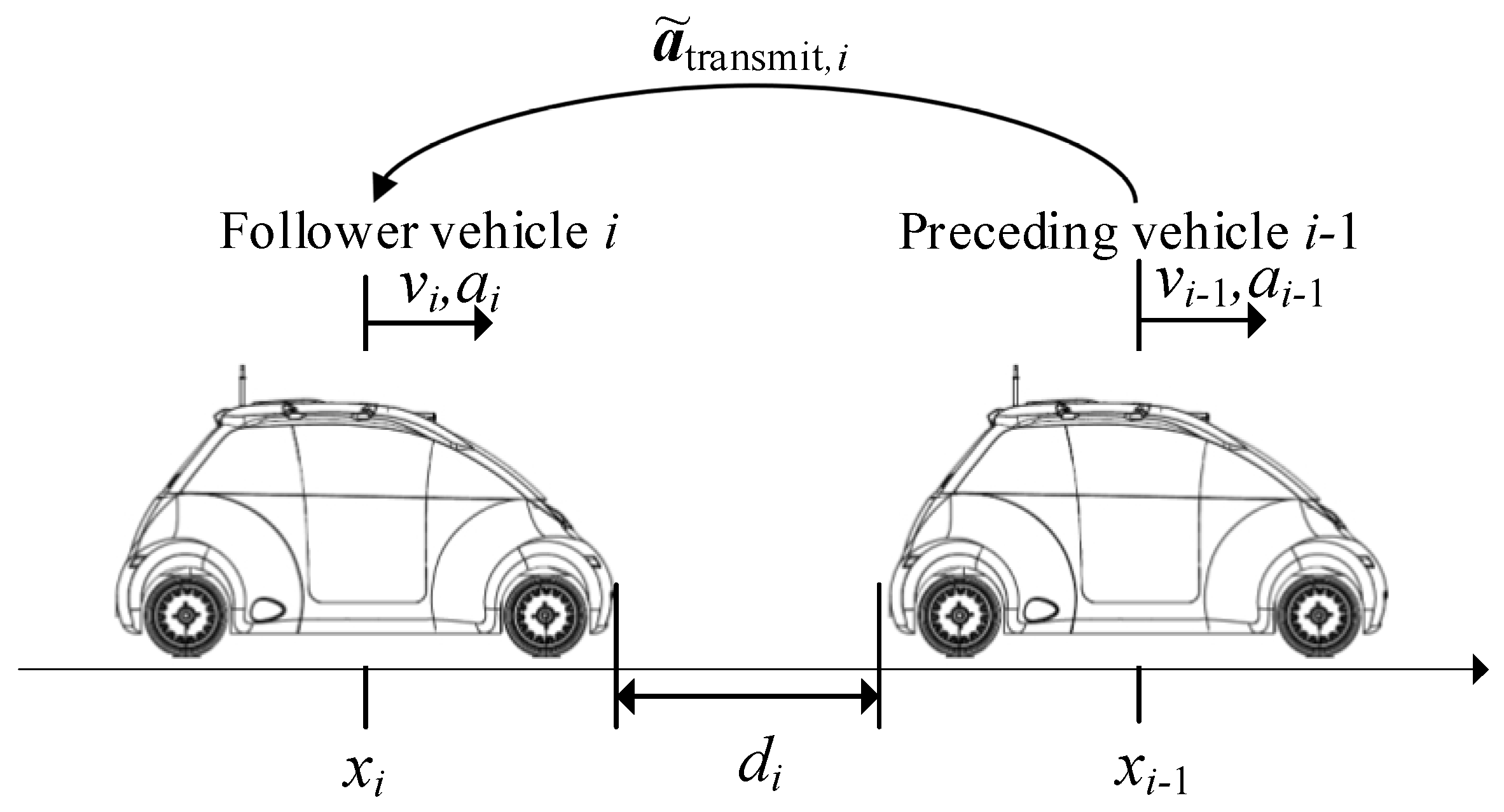
Figure 1 shows the follower vehicle with index
i driving behind the preceding vehicle with index
i − 1, separated by the bumper-to-bumper distance
. Both feature their corresponding position
, velocity
and acceleration
. The entire platoon is composed of
vehicles.
The target distance
to the preceding vehicle may be decribed via a constant spacing or constant time-headway [
1], with constant time-headway being defined as [
26]:
where
denotes the distance at standstill and
denotes the variable distance, adjusted by the time-headway
. The deviation from the target distance is described by the distance error:
Analyzing string stability is more difficult in DRL than in a model-based approach, because the DRL problem is not typically designed in a frequency domain, where string stability usually is easier to analyze [
26,
27]. In [
28], it was shown that string stability can be guaranteed as follows:
where
is the acceleration of the respective vehicle in frequency domain.
2.1. Communication Model
Regarding the platooning C2C information flow, a predecessor-following topology (cf. [
3]) was adopted: in such a topology, information is sent one way from the preceding vehicle to the following vehicle (cf.
Figure 1).
For modeling the communication, an appropriate distance for transmitting data and a sufficient signal bandwidth was assumed. For a specific prediction horizon
, the preceding vehicle
transmits its current acceleration and its predicted accelerations over a
-window
. For
, only the current acceleration is transmitted. The follower vehicle receives the delayed acceleration
with an assumed delay of
for vehicle
(cf.
Table 1).
In this communication, burst errors due to noise may occur, and a sequence of successive transmissions
is not received. The burst errors are modeled with a Markov chain according to the Gilbert–Elliot model [
29] (cf. [
30],
Figure 2). The Markov chain consists of a state
, which can receive transmissions, and a state
, in which transmissions are unavailable. According to the Markov property, the transition to the next state only depends on the present state. This means that for state
, it remains in state
with probability
and
or leaves it with
. The same holds true for state
with
and
. The Markov chain was implemented as an automaton, starting in the receiving state. The probabilities used for the automaton in case of the occurrence of burst errors were taken from [
30]. They parametrized a low communication quality, and can be found in
Table 2. A parametrization for perfect communication quality is also given.
Reference [
30] suggested the use of a buffer when a sequence of prediction values is transmitted. The buffer is referred to as
. For each time step
, the received transmitted acceleration
is saved in the buffer:
. If a burst error occurs, no
is received. In this case, the first element of the buffer no longer contains valid information and the resulting gap in the buffer is filled with a placeholder
(cf.
Table 1).
is an invalid acceleration value that was chosen to be large enough not to be attainable in our scenario, such that it could not occur in regular communication, and was interpretable as a communication error by the DRL agent.
2.2. Vehicle Model
The single vehicle was created as a two-track model in Modelica [
31] using Dymola [
32] and the planar mechanics library [
33]. Modelica is an object-oriented open source modeling language for multiphysical (e.g., mechanical and electrical) systems. The vehicle model represented the properties of the ROboMObil (ROMO) [
34], which is the robotic full x-by-wire research vehicle of the German Aerospace Center (cf.
Figure 1 for two ROMOs forming a platoon). The center of gravity (used to calculate the vehicle’s position
; cf.
Figure 1) was assumed to be at the geometric center of the rectangle spanned by the track width and the wheelbase.
As wheel models, four dry-friction slip-based wheels of the planar mechanics library [
33] were used and connected to fixed translation elements. The slip-based wheels limited the amount of propulsion force dependent on the normal force and the friction coefficient.
The energy consumption of the single vehicle mainly depended on the variable air drag and the electric powertrain.
ROMO’s surface front
, air drag coefficient
and the air density
were chosen according to [
35] (cf.
Table 1). Reference [
36] stated that the air drag coefficient is dependent on the distance
to the preceding vehicle: When driving close to the preceding vehicle, the air drag coefficient is reduced. This reduced air drag leads to less power being necessary for driving. To model the variable air drag, a nonlinear approximation was used, as suggested by [
37]:
where
and
are variable air drag function coefficients. The parameters were obtained by performing a linear regression on the experimental data given in [
38]. The variable air drag force can then be calculated as:
The battery of one single vehicle [
39] consist of
cells connected in series (cf.
Table 1). The total pack voltage
and total pack resistance
were assumed to be constant during experiments (at 100% state-of-charge). To account for battery losses, we considered Ohmic heat losses in each cell (each cell with respective voltage
and resistance
).
Each of the four wheels was powered by an in-wheel motor, which was modeled as an open-loop controlled permanent magnet synchronous machine [
35,
39,
40]. This allowed us to calculate the vehicle’s power consumption
as:
where
is the summed mechanical power of all electric motors. For each
-th motor (
),
, with motor torque
and mechanical rotor angular velocity
.
also considered the powertrain losses
, which consisted of the Ohmic heat losses in the battery and the losses in the electric motors (i.e., inverter losses, copper losses, iron losses, and mechanical friction losses).
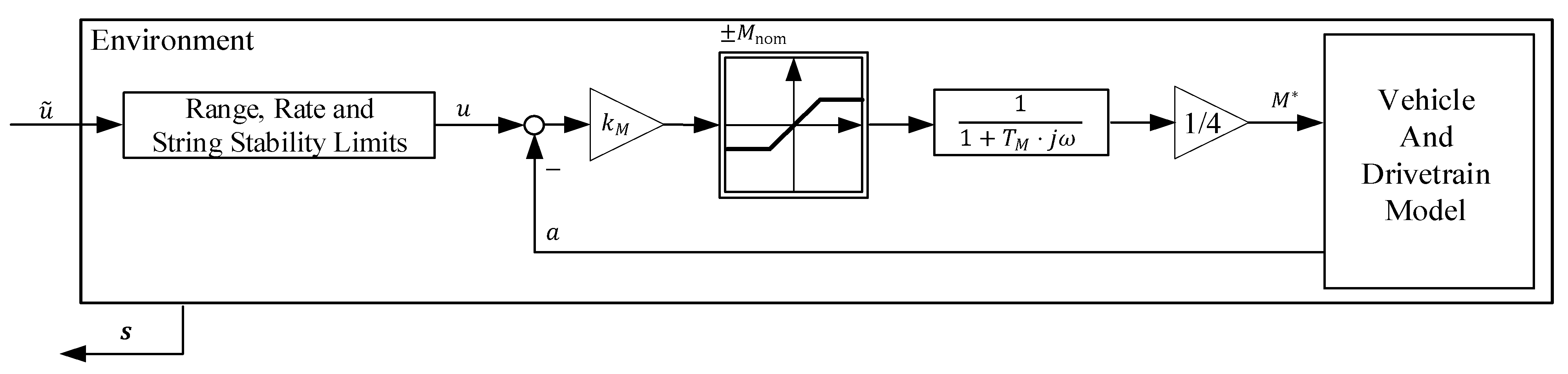
A proportional controller was used as the low-level acceleration control (with a high gain
), which controlled the torque set point
for the electric motors. The torque was limited to
(nominal torque, cf.
Table 1), so that the physical constraints of the system were not violated. Additionally, a first-order low pass filter was applied to the acceleration control’s output with a time constant
to achieve an actuator lag.
The block diagram in
Figure 2 gives an overview of the used vehicle model with respect to the RL framework discussed in
Section 3 (cf.
Section 3.2 for more information on action
, denormalized neural network output
and the respective range, rate and string stability limits; cf.
Section 3.3 for more information on feedback state
).
2.3. Leader Vehicle Motion Model
For modeling the platoon’s leader vehicle motion, trajectory data from the Next Generation Simulation (NGSIM) dataset was used [
41]. In this dataset, positions of vehicles were measured with multiple synchronized cameras at different locations in the USA (Emeryville’s Interstate 80; Los Angeles’ Route 101; and Lankershim Boulevard, Atlanta’s Peachtree Street) at two to three specific times of the day. In doing so, it was aimed at portraying different amounts of traffic and thereby different vehicle trajectories during the buildup of congestion, during transition between congested and uncongested traffic, as well as during full congestion.
The NGSIM data must be postprocessed due to measurement errors [
42] to create consistency between velocity and acceleration signals. In this work, this was done in a multistep approach by:
Removing acceleration outliers () by applying a natural cubic spline interpolation on the velocity profile;
Reducing the velocity profile noise by applying a first-order low-pass Butterworth filter (cutoff frequency of 0.5 Hz); and
Removing implausible accelerations ( or ) also by applying a natural cubic spline interpolation on the velocity profile.
Finally, if implausible accelerations were still present or if velocities higher than ROMO’s nominal velocity limit occurred, the trajectory was removed from the set of valid trajectories. After doing so, the resulting set consisted of 312 trajectories. It was permutated and then split into training (70%) and validation (30%) sets.
3. Reinforcement-Learning-Based Cooperative Adaptive Cruise Control
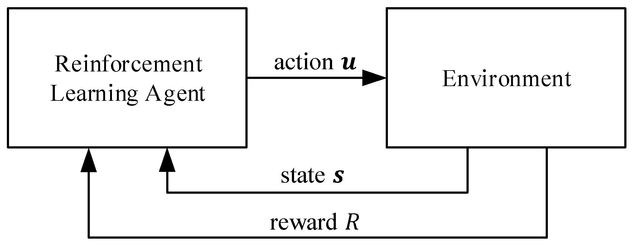
In this work, we used reinforcement learning to solve the control problem. A Markov decision process (MDP) described the probabilistic basis of RL, and was used to derive the algorithms to find the optimal action in each time step. An MDP consists of an agent and the environment, as shown in
Figure 3. In each discrete time step
, the agent perceives the current state
(
being the set of all valid states) of the environment and performs the corresponding action
(
being the set of all valid actions) [
5]. If a reward
is assigned according to the action
and the resulting state
, the MDP can be called a Markov reward process (MRP) [
43]. The MRP is defined to begin with state
and action
, but without an initial reward. The first reward
is assigned after the transition to the state
. From a control theory’s perspective, the agent can be seen as controller, the environment as plant, and the action as control signal.
A sequence beginning with
and ending with a terminal state
is called an episode
[
5]. After reaching
, no further action can be taken and a reset to a starting state occurs. In this work, a fixed interval between action and new state
(cf.
Table 1) was assumed, yielding the time
with
.
For the MDP, the Markov property also held true (cf.
Section 2.1).
3.1. Policy Optimization
The policy
describes which action an agent takes given a certain state. This can be described with a stochastic policy
as in [
43]:
The agent tries to maximize the discounted return
which is the sum of rewards that are received until the terminal state is reached, each multiplied by a discount factor
[
5]:
In the case of
, the discounted return was just referred to as return in this work. The state-value function is defined as the expected discounted return for a state
when a given policy
is applied:
The goal of RL is to find the optimal policy
that optimizes the expected discounted return for a specific episode
(with the actions of
being taken according to
):
Regarding DRL, this work used the proximal policy optimization (PPO) algorithm with clipping [
44,
45] to calculate neural-network-based approximations of
and
. The weights of the neural network [
46]
are referred to as
,
and
.
PPO uses gradient ascent to optimize
, such that the obtained discounted returns following a state-action tuple (
) are more probable. These obtained discounted returns are described with the estimated advantage
[
5,
44,
47]. PPO does not directly optimize the policy, but it uses an objective function
[
44]:
with:
where
is the probability ratio
and
is the clipping function. The clipping function limits the changes of
to [
]. Thereby, the objective function
creates an incentive for only small changes of
, which increases training stability compared to a basic DRL algorithm (in this work, training stability meant a monotonic increase of the obtained average returns during training).
The basic principle of operation of PPO is shown in Algorithm 1. As for the policy, the update of the value function
(step 11) can be performed via gradient descent, such that the objective function
is optimized. Policy and value function updates are repeated in multiple passes until the trained policy’s behavior converges, which means until the obtained returns can approximately no longer be increased.
| Algorithm 1. Basic PPO principle of operation [44,45,47]. |
| 1: | Input: initial policy parameters , initial state-value parameters |
| 2: | repeat: |
| 3: | for each process i with i = 1, …, n: |
| 4: | Generate |
| 5: | for each transition with k = 1, …, T: |
| 6: | Compute |
| 7: | 1 |
| 8: | end for |
| 9: | end for |
| 10: | Update the policy by maximizing the objective function L |
| | in training epochs, sampling a minibatch (with |
| | n·T/nmini transitions) in each epoch |
| 11: | Update the value function |
| 12: | until convergence |
| 13: | Output: trained policy , trained state-value function |
| 1 Different advantage term calculations are possible. |
The computational time of the training is decreased by using multiprocessing with n processes. For this, each process i is used to generate T transitions with a shared policy .
The policy is updated in passes (called training epochs) for each pass of the PPO algorithm. For each update of in an epoch, a minibatch consisting of multiple transitions is sampled. The minibatch is a subset of the batch of n·T transitions that is available in each pass of the PPO algorithm. The size of the minibatch is defined by dividing the size of the batch by the minibatch scaling factor . The number of passes until the algorithm converges is estimated by defining a fixed training length, which means the total number of generated transitions after which the training is ended.
3.2. Actions
The agent controls a follower vehicle (i.e., it acts with the environment) by setting a target acceleration
. To improve passenger comfort, a jerk limit is introduced to enforce action smoothness:
with
= 0.5 m/s
2 and
. The action
is the denormalized output of the policy
. Furthermore, only accelerations that are within the physical limits of the car are allowed to be set:
In this work, the following two assumptions were made:
To satisfy assumption 1, the low-level acceleration controller was assumed to provide an accurate tracking performance. To satisfy assumption 2, the acceleration of the preceding vehicle
was assumed to be approximately equal to the delayed acceleration
that was received by the follower vehicle (cf.
Section 2.1). When we transferred the string stability concept of (3) to time domain with:
this allowed us to represent the string stability condition as:
In (15), the acceleration of the follower vehicle
must be smaller than
times the maximum acceleration of the preceding vehicle within a string stability time window
for every time step
. Thus, the follower vehicle is assumed to mimic the driving behavior of the preceding vehicle. If it does so and the accelerations are mostly attenuated downstream, string stability is guaranteed to a given extent. The transfer of the string stability concept (3) to time domain (15) was proposed in a similar way in [
28].
Equation (16) makes the implementation of a string-stability condition easier, as it is not necessary to abort the episode due to a state constraint violation: only an additional control limit must be added. The resulting maximum from (16) is referred to as string-stability limit . Furthermore, only valid values of are taken into consideration, and cannot be below = 0.1 m/s2. gives the agent the possibility to counteract slight perturbations.
In this work,
= 20 and
= 0.999 were chosen. With the fixed time interval
(cf.
Table 1) between two steps
and
, this meant that the current acceleration and the received accelerations from the past two seconds were taken into consideration.
3.3. Feedback State
The design of the CACC DRL environment considers a two-vehicle platoon. The motion of the first vehicle—the leader—followed a reference trajectory obtained from the NGSIM dataset (cf.
Section 2.3). The motion of the second vehicle—the follower—was controlled by the DRL agent. The follower vehicle was referred to with index
, the leader vehicle with index
. The agent state vector
of the follower vehicle for time step
was chosen as
The states were partially chosen with respect to (1), with
being the velocity of the vehicle and
being the acceleration of the vehicle.
is the distance to the preceding vehicle:
with
being the position of the respective vehicle and
its respective vehicle length.
is the discrete approximation of the distance dynamics
at time
.
is the distance error (cf. (2)) and
the power consumption at time step
(cf. (6)). Even though we did not investigate if this state selection fulfilled the Markov property, assembling the feedback state this way provided the agent with rich information about the environment.
The state
was augmented with the history of past control values (as suggested by [
48]) for learning a smooth control action. For this purpose, the actions from the prior two time steps
and
were provided.
The state was normalized before it was fed into the policy to ensure the agent considered each state component equally.
3.4. Reward Function
The control goal of string stability is targeted by the action limit (16), while the jerk limit (13) ensures at least a certain degree of passenger comfort. The control objective of maintaining a safe distance while reducing air drag is incorporated into the CACC environment through the reward function.
To enhance the passenger comfort besides the already constrained change in control value (cf. (13)), was also penalized in the reward function.
The reward function was defined in such a way that it was always negative:
If the episode was not aborted, the weighted () and normalized ( error , power consumption and action change created the achieved reward. The normalized state components and actions were used.
Several conditions led to a premature end of an episode and were related to safety and error constraints. To not crash into the preceding vehicle, the distance must always be larger than 0 m. Additionally, we chose an upper distance limit of 50 m:
At the same time, this limited the maximum platoon length, thereby increasing the road capacity. To increase safety, the relative velocity also was limited:
If the episode was aborted, a negative reward
was assigned. The trained state-value function
contained the information on whether specific states most likely were going to lead to a premature end of an episode (leading to a low return). Via the estimated advantage
, this was learned by the agent during training (cf. (11)). This meant that for example the agent already attempted to avoid distances
larger yet close to
.
Maximizing the reward function yielded the desired behavior: error minimization, minimization of the power consumption, and an enhanced ride comfort by providing a smooth target acceleration signal. Two different sets of reward weights were heuristically determined and are listed in
Table 3. The error-minimizing weight set (EM-RL) focused on minimizing the error
, while the power-minimizing weight set (PM-RL) also explicitly considered the minimization of the absolute power consumption
. The minimization of
aimed at reducing the consumed energy
at the end of the episode
:
. Even though recuperation was possible, every acceleration and deceleration led to additional losses. Therefore, the less acceleration and deceleration was performed, the less powertrain losses occurred (smaller
), which yielded a smaller energy consumption
.
In case of PM-RL, the weight for the error penalization was reduced to enable the agent to focus less on the error and thereby to deliberately deviate from the set point distance to reduce . In the case of EM-RL, the weight was set to zero, which was why the power was not explicitly considered.
4. Simulative Assessment
PPO was deployed with a policy network of two hidden layers with 64 neurons, each with the
activation function and using the Adam optimizer [
49]. The default hyperparameters [
45] were used, and
n = 4 parallel processes
were utilized to achieve a lower computational time of the training. The minibatch scaling factor was increased from the default value
to
to create smaller minibatches and thereby further reduce the computational time (cf. Algorithm 1 and its description in
Section 3.1). Since the default hyperparameters provided good training results, no further effort to optimize the hyperparameters was spent.
Training with the EM-RL reward function was performed with a batch size of 4⋅128 steps (
T = 128 steps per process were used as defined as default in [
45]) and a training length of 2 × 10
6 time steps. Training with the PM-RL reward function was more complicated due to the added control goal of power minimization. This is why the batch size is increased to 4⋅256 steps (
T = 256) to stabilize the training. On the one hand, this led to a lowered sample efficiency, as more samples needed to be assessed before the policy is updated. On the other hand, the information from more samples was averaged before an update, leading to the policy being less prone to converge to local optima. As this also slowed the training process, the training length was increased to 4
10
6 time steps. See
Appendix C for information on average run times.
The training outcome changed based on the initial random seeds (i.e., numbers used to initialize pseudorandom number generators), which affected the randomly assigned initial neural network weights, as well as the environment initialization. A reproducible training setup is a known issue in DRL [
50]; to this end, several seeds should be used in each training. The authors of [
50] suggested the use of at least five seeds; in this work, nine differently seeded runs were performed for each reward parametrization and communication parametrization. For analyzing the training, the mean return and the standard error were calculated in bins of 50,000 time steps for all training runs.
The DRL environment was created in the Python-based DRL framework OpenAI Gym [
51], which provided standardized interfaces to connect DRL environments with DRL algorithms. The Modelica model of the vehicle was exported as a functional-mock-up unit (FMU) [
52]. The software package PySimulator [
53,
54] was used to connect to the FMU and to create a Python-based interface, which could then be directly addressed by the DRL environment. This toolchain was first applied by our group in [
9].
4.1. Training
Each CACC environment was initialized with a processed NGSIM velocity and acceleration trajectory. The trajectories were sampled from the NGSIM training set. A training episode had a length of
(cf.
Table 4), if it was not aborted earlier.
The initial velocity of the follower vehicle was selected as
where
was limited to be not below 0 m/s.
With
,
can be calculated according to (1). The initial distance
is defined to be equal to
plus a value
:
was limited to be not below
. The initial values, as well as the sampling intervals (sampling performed with continuous uniform distribution) of
and
can be found in
Table 4.
The random initialization of and as well as the random sampling of a leader vehicle trajectory, aimed at forcing the agent to cope with a wide variety of initial states and the avoidance of overfitting. Randomly initializing the environment helped the agent to explore the state space, which was inherently considered by the algorithm by using a stochastic policy during training.
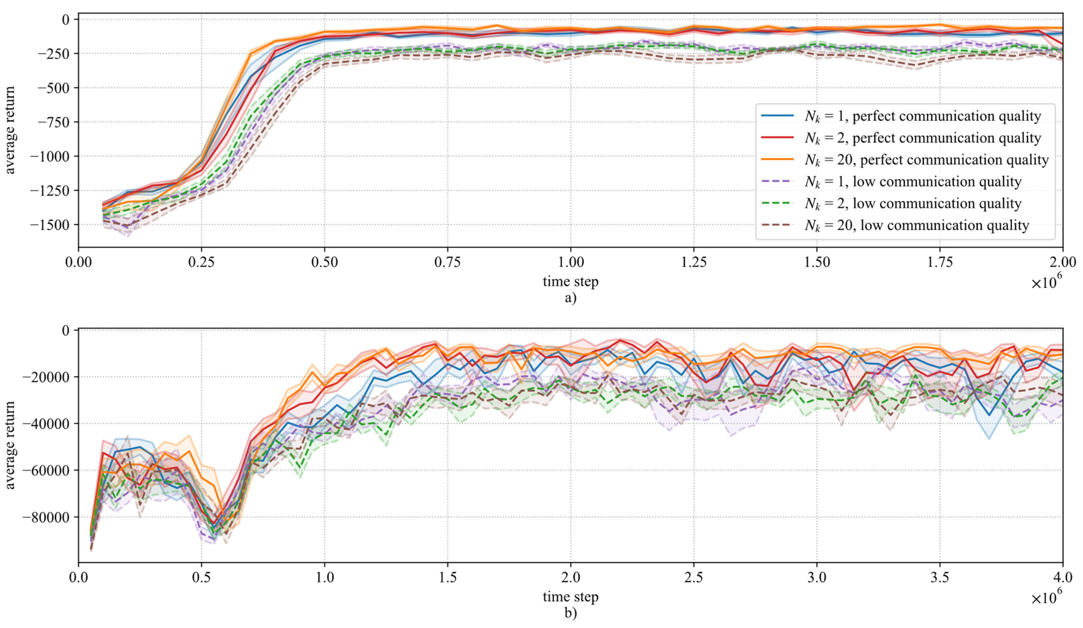
The training results for different prediction horizons
, training communication qualities, and reward functions are shown in
Figure 4.
The training evolution with the EM-RL reward function is depicted in
Figure 4a. One can see a stable training behavior, with a low standard error for all trainings. The average return converged at approximately 0.5 × 10
6 time steps. Initially, the average return was below
= −1000, because the agents explored different policies, and many lead to an episode being aborted. Comparing the curves for perfect communication quality with prediction horizons
= 1, 2 and 20, one can see that there was a slight increase in sample efficiency (i.e., convergence speed w.r.t. time steps) for higher prediction horizons, and all prediction horizons showed good training stability. This suggested that the agent could make use of the additional information provided by an increased preview.
The training with low communication quality showed a drop in average return, and the training performance was worse regarding the achieved final average return. Since the agent only had access to less reliable information, the achievable performance was reduced. This could also be observed for PM-RL.
The PM-RL weight set led to higher absolute rewards due to the nonzero weight
compared to the EM-RL weight set, as can be seen in
Figure 4b. Additionally, it showed a less stable training behavior. Therefore,
was increased (cf.
Table 3) to ensure that the agent focused on the safety and error constraint (cf. (20) and (21)).
The average return rose during the first 0.2 × 10⁶ to 0.5 × 10⁶ time steps. After reaching a peak, the return dropped and rose again shortly after until convergence. This can be explained by the opponent reward terms regarding the error and the power consumption : by following the leader vehicle but accelerating with lower absolute amplitude than it, the agent could easily decrease . However, at the same time, this increased . Only by exploration and considering the possible air drag reduction could a policy be found that reduced both and .
The general occurrence of training instability of PM-RL compared to EM-RL might have been created by including both the power consumption and the change in control value in the reward function: The penalized power consumption could also reward control value smoothness, even though this was not its actual aim. Therefore, this created an ambiguous goal for the optimization.
When comparing the PM-RL curves for perfect training communication quality with prediction horizons = 1, = 2, and = 20, one can see that there was an increase in sample efficiency after 0.7 × 10⁶ time steps for = 2 and = 20. This showed that the additional information acquired through the prediction horizon increased the training performance.
4.2. Test Set Evaluation
For validating the performance of the EM-RL and the PM-RL agents, they were compared to a model-based proportional-derivative (PD) controller, extended with a feedforward (FF) element to incorporate transmitted acceleration information [
26] (cf.
Appendix A for more information). This controller was referred to as a model-based PDFF (mb-PDFF) controller, and was applied to the test set with both reward function parametrizations. It was also implemented in Modelica/Dymola, like the vehicle model.
Because the design of the mb-PDFF from [
26] did not consider any preview; i.e., only the present acceleration was transmitted, the mb-PDFF was exclusively compared with DRL results with a prediction horizon of
= 1.
For evaluating the performance of the trained policies, they were deterministically applied on the test set. For this, the random initialization was turned off; i.e., and (cf. (22) and (23)).
It was necessary to select a specific agent out of the set of trained agents to make a direct comparison, as only a single agent could be used as controller in the follower vehicle. The policies with the least amount of crashes in the test set were selected. For training with perfect communication quality, only the test set results with perfect communication quality were considered. For training with low communication quality, the test set results with both perfect and low communication were considered, because the trained agent was expected to perform well in both situations. In case of the same number of crashes, the agent with a higher mean return in the test set was selected. is defined as , with being the number of episodes that were not aborted in the evaluation of the test.
Table 5 shows the policies corresponding to the best performing runs for each of the reward function parametrizations and communication qualities. The shown DRL evaluation results were obtained with perfect communication quality. In addition to the number of test set aborts, the mean energy consumption:
and the root mean squared error:
were evaluated. The
was calculated with respect to the episode steps
that corresponded to
.
First, mb-PDFF was compared with EM-RL and PM-RL, each trained with perfect communication quality (P-EM-RL, P-PM-RL).
The P-EM-RL agent showed the best performance with respect to the minimization of . The P-EM-RL showed a much smaller than mb-PDFF (−78.7%). This can be explained by model uncertainties being considered in the design of the mb-PDFF, which made the mb-PDFF less aggressive in order to be capable of adjusting to parameter deviations. Additionally, the P-EM-RL had a lower (−9.9%) than mb-PDFF, because the P-EM-RL was trained to minimize the change in control value.
P-PM-RL was able to reduce by 17.9% compared to mb-PDFF and 8.9% compared to P-EM-RL. One can see that the deliberate deviation from the set point distance was used to decrease the power consumption, and thereby decrease the energy consumption. This also led to a significant increase in the distance error: P-PM-RL’s was 3.6-fold larger than mb-PDFF’s, and 17.1-fold larger than P-EM-RL’s.
Subsequently, EM-RL and PM-RL trained with low communication quality (L-EM-RL, L-PM-RL) were considered. Both L-EM-RL and L-PM-RL performed similarly to their counterparts P-EM-RL and P-PM-RL, but slightly worse (L-PM-RL had a lower than P-PM-RL, but a higher ). This can be explained by the occurrences of burst errors during training, which made the agents rely less on the transmitted acceleration information.
This led to L-EM-RL being less capable of reaching the set point distance than P-EM-RL, while simultaneously having an increased . Similarly, this led to L-PM-RL being more careful with deliberately deviating from than P-PM-RL, and therefore also having an increased .
For all DRL agents, one test set abort occurred out of the 93 tested trajectories. This was related to the strict string-stability implementation of the DRL agents (as opposed to only considering string stability during the tuning of the mb-PDFF’s parameters, cf.
Appendix A) even in emergency breaking situations.
The evaluation results for higher prediction horizons (
and
) are summarized in
Appendix B (cf.
Table A2; the DRL results in
Table 5 are an extract from
Table A2).
Larger prediction horizons only partially yielded a better performance of the agents. Only yielded a lower for P-EM-RL, while neither nor improved L-EM-RL’s performance. This can be explained by the set point distance tracking problem to be sufficiently solvable with . At the same time, an increased prediction horizon meant for the agent to identify the superfluous information, and therefore increased the difficulty. This was especially true for low communication quality, for which correct acceleration information was partially not available.
For P-PM-RL, a prediction horizon increase from to led to a lower , while stayed approximately the same. A further horizon increase from to led to a lower and (w.r.t. perfect communication quality during evaluation). For L-PM-RL, an increased prediction horizon led to a lower , but a higher . This showed that even for low communication quality, the energy minimization objective benefited from a larger prediction horizon.
Overall, training with low communication quality resulted in a policy that was more robust regarding and during low communication quality. However, the agents trained with low communication quality also showed multiple test set aborts during evaluation with low communication quality.
4.3. Controller Analysis
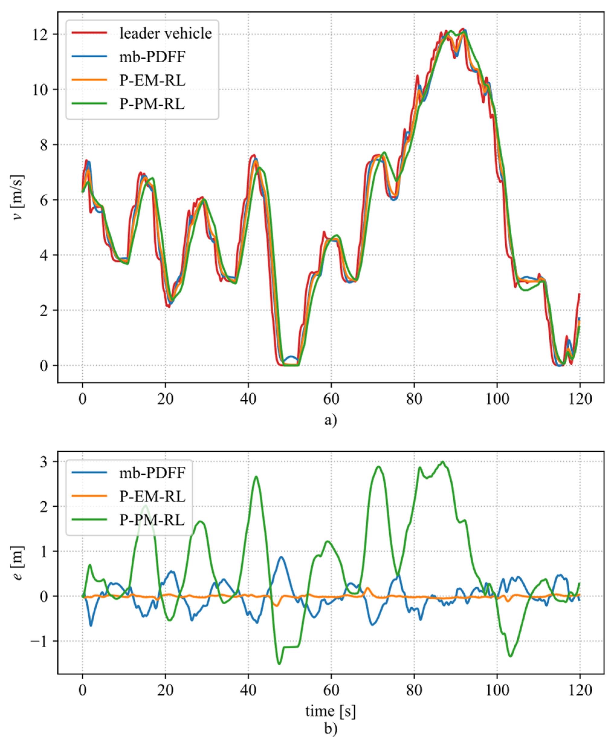
In the following section, the mb-PDFF, P-EM-RL, and P-PM-RL (the latter two with a prediction horizon of = 1) are analyzed in time domain with one trajectory chosen for the leader vehicle.
Figure 5a shows the velocity of the leader vehicle, as well as the velocity of the follower vehicle, as it was created by the mb-PDFF, the P-EM-RL agent, and the P-PM-RL agent. The good performance regarding the distance error minimization of P-EM-RL is clearly visible in
Figure 5b.
It can be seen in
Figure 5a that the follower vehicle mimicked the driving behavior of the leader vehicle. P-PM-RL showed undershoots after longer periods of deceleration (e.g., at 105 s), which resulted from deliberately deviating from the target distance
(cf.
Figure 5b). Before the undershoot, P-PM-RL drove faster than the leader vehicle. At the end of the deceleration phase, the follower vehicle drove closer to the preceding vehicle to benefit from the reduced air drag. Afterwards, the reduced distance was compensated by driving slower than the leader vehicle, which meant by performing an undershoot. It should be noted that these undershoots resulted in negative velocity in the case of the preceding vehicle’s velocity approaching 0 m/s (e.g.,
Figure 5a at 50 s). This behavior was possible during training and driving cycle set evaluation, but was forbidden here in the time domain analysis.
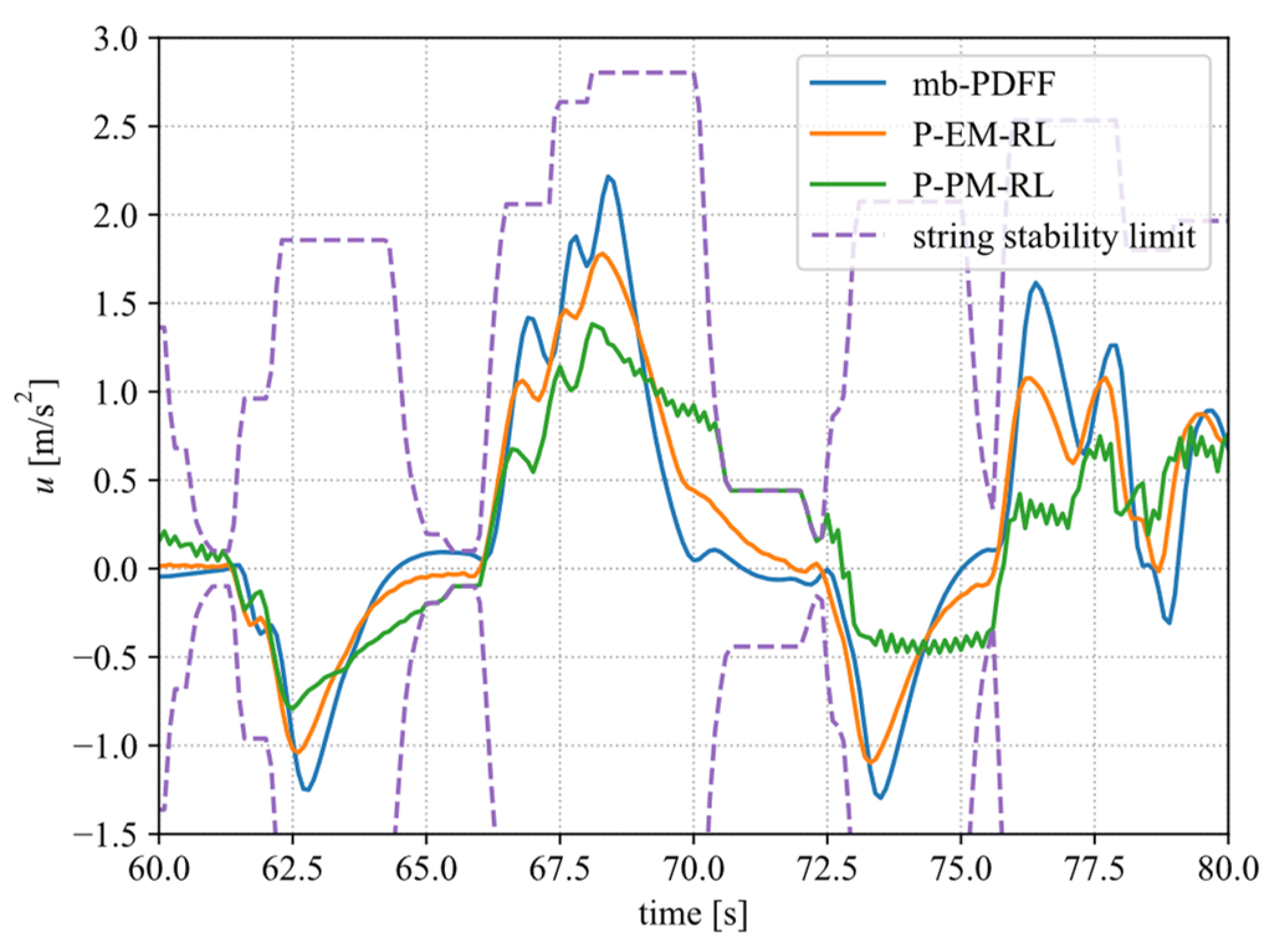
Figure 6 shows the control value
for mb-PDFF, P-EM-RL, and P-PM-RL for the time interval of 60 s to 80 s of the episode (the time interval was well suited to show the characteristic controllers’ behavior and the effect of the string-stability limit). It can be seen that the amplitude of P-EM-RL was lower than that of the mb-PDFF, which most likely was caused by the penalization of the change in control value
in its reward function. This showed that the P-EM-RL was less aggressive in general than the mb-PDFF (leading to a lower energy consumption), while having a better error-minimizing performance (cf.
Table 5 and
Figure 5b).
Regarding the constraints, the figure shows that the control value of the mb-PDFF and both agents remained within a modest range (cf. (14)), that the DRL agents respected the string stability limit, and that, usually, the mb-PDFF also was compatible with the DRL agents’ string-stability limit.
The P-PM-RL agent still shows a nonsmooth signal due to the ambiguity created by penalizing both the power consumption and the change in control value. During periods of acceleration and braking, it showed lower maximum absolute accelerations, but higher absolute accelerations at the end of the periods than mb-PDFF and P-EM-RL. This allowed it to deviate from the target distance .
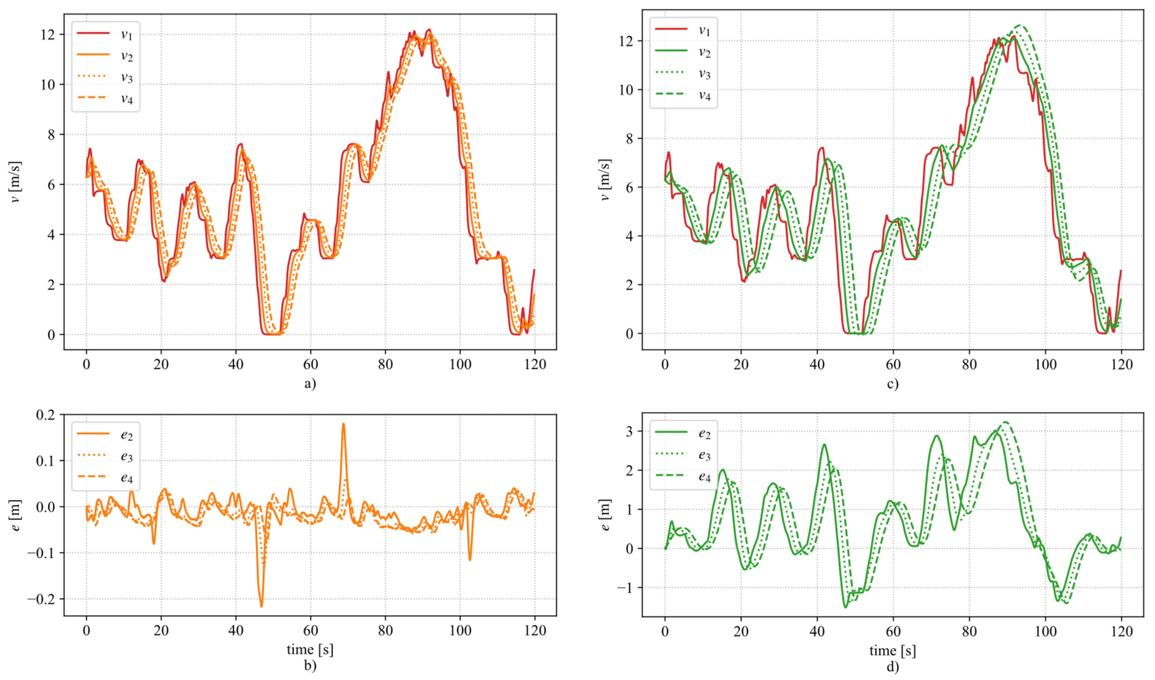
For analyzing the trained agents’ string-stability property, a platoon with three P-EM-RL-controlled follower vehicles was simulated (
Figure 7a,b) and three P-PM-RL-controlled follower vehicles (
Figure 7c,d) (P-EM-RL and P-PM-RL both with prediction horizon of
).
The P-EM-RL-controlled follower vehicles behaved as string stable: each follower vehicle followed the preceding vehicle without an acceleration amplification downstream. This also led to a reduction of the maximum absolute distance error values, as can be seen in
Figure 7b at 50 s, 70 s, and 105 s.
The P-PM-RL-controlled vehicles mostly behaved as string stable, but also showed instabilities. The velocity over- and undershoots with respect to the preceding vehicle were amplified downstream at 90 s and 105 s, such that the absolute distance error also was amplified. For negative distance errors, this may lead to a crash. This was not fully prevented by the string stability limit (cf. (16)), because it only referred to the maximum absolute acceleration value of the preceding vehicle within the string stability time window , but not the duration of this maximum acceleration. Thus, in future work, the string-stability limit also needs to restrict the acceleration duration of the follower vehicle. Additionally, this reduction of possible acceleration amplitude would increase the passenger comfort.
The string stability behavior of the P-EM-RL-controlled vehicles also suggested the assessment of P-EM-RL-controllers in platoons with more than three agent-controlled vehicles, whereas the P-PM-RL-controllers first required a stricter string-stability limit.
5. Discussion and Outlook
This work assessed the use of deep reinforcement learning for CACC.
A buffer was used in the C2C communication to store the predicted acceleration information. This enabled the use of a prediction horizon of multiple future time steps. The occurrence of burst errors was modeled with a Markov chain, and burst errors were marked as invalid information in the buffer. Furthermore, a string-stability condition was incorporated by limiting the acceleration set point of the follower vehicle with respect to future accelerations of the preceding vehicle. Thereby, accelerations could not be amplified downstream in the platoon without limit.
If the training and application of deep reinforcement learning is not properly designed, robustness and overfitting problems might occur; i.e., the learning-based algorithm is highly optimized for the data synthetically generated during simulation, failing to cope with data generated by the real system. This is particularly worrisome when transferring the algorithm from a simulation environment to the real world, leading to potential loss of performance (best scenario) and safety (worst case). To mitigate these issues in our work, model randomization techniques were incorporated into the learning process. The key idea was to inject parameter variability in the simulation model, exposing the agent to model inaccuracies during the learning phase, yielding robust control policies. In our work, particular attention was dedicated to exposing the control algorithm to different levels of communication delays and errors, one of the main sources of uncertainty in the platooning applications.
Multiple agents were trained and evaluated on an extra test set that was not used for training. The best performing agents were validated by comparison with a model-based PD controller with feedforward. Here, the distance error minimizing CACC agent was able to outperform the model-based controller by reducing the by up to 78.7% on the test set.
In comparison with the model-based controller, the energy minimizing CACC agent reduced the mean energy consumption by 17.9% on the test set. For the error-minimizing agents, it was shown that only small increases of the prediction horizon length yielded a better error minimization, whereas the energy consumption could also be improved by large increases of the prediction horizon length. Moreover, it was shown that considering burst errors during training created an agent that was robust against them and performed well regarding distance errors and energy minimization.
All in all, it was possible to train agents that could: (1) minimize their energy consumption; (2) provide string stability to a given extent; (3) exploit preview information available in the communication; and (4) minimize the effect of burst errors.
However, to guarantee string stability more generally, the string stability limit should be able to change depending on the driving situation. Most of the time, it should be stricter, and also should consider the acceleration duration of the preceding vehicle instead of only the maximum acceleration. During test set evaluation of the DRL agents, some test set aborts occurred due to the string-stability limit in emergency breaking situations. Thus, the string-stability limit should also be less restrictive when the distance to the preceding vehicle is very low.
The experienced predisposition of DRL towards unsmooth control signals is a disadvantage, and must be considered when transferring the controller to real-world applications. Unsmooth acceleration control signals lead to high jerks and reduce driving comfort. In addition, they increase energy consumption.
In the future, we plan to validate the obtained results with experiments on real-word vehicles.


