Trajectory Optimization Algorithm for a 4-DOF Redundant Parallel Robot Based on 12-Phase Sine Jerk Motion Profile

Abstract

To improve high motion accuracy and efficiency in the high-speed operation of a 4-DOF (4 degrees of freedom) redundant parallel robot, this paper introduces a trajectory planning of the parallel robot in joint space based on the twelve-phase sine jerk motion profile. The 12-phase sine jerk motion profile utilizes the characteristics of a sine function. Furthermore, the penalty function is used to optimize the trajectory energy consumption under the constraint condition. The simulation and experimental results show that the energy consumption of joint space is slightly higher than that of the three-phase sine jerk motion profile, but the overall operation is more accurate and stable. Specifically, the sudden change of force and velocity in each joint is eliminated, which is the cause of mechanism oscillation. Moreover, the force of each joint is more average. The results indicate that each movement is closer to the maximum allowable limit and the running efficiency is higher.

1. Introduction

The 4-DOF redundant parallel robot is widely used in industrial production lines. It has the advantages of good rigidity, high movement precision, and compact structure [1,2,3,4,5,6]. Thus, it is especially suitable for the operation of lightweight objects, sorting and packing in high-speed handling, etc. [7,8]. The inertia of the robot arm, however, causes vibration and jerk when the robot moves at high speed, leading to the low accuracy and stability of the robot. Scholars have carried out in-depth research from the point of trajectory planning. For example, in Reference [9], the three-phase sine jerk motion profile was used as trajectory planning to reduce the jerk caused by the high-speed point-to-point motion of the robot. Fang et al. [10] proposed a method of expanding the three-phase sine jerk motion profile into a fifteen-phase sine jerk motion profile. Based on the research of Li and Fang, with the limit of each joint of the robot motion, Valente et al. [11] proposed a multivariable time optimization method to plan the optimal trajectory of joint space on the three-phase sine jerk motion profile and made the running time of the trajectory shortest. To reduce the computation load of trajectory planning for online calculation of trajectory planning, some researchers adopt the method of piecewise interpolation. Wang et al. [12], based on the three-phase sine jerk motion profile, constructed a new compound sine trajectory to realize the online fast interpolation feature of joint space motion trajectory, through using polynomial transition interpolation at the beginning and end of joint motion.

However, with the acceleration of the speed of the robot, the energy loss in the running process has become a non-ignorable problem. Therefore, some scholars began to discuss the possibility of robot trajectory optimization from the point of energy and to obtain many valuable research results on the optimization algorithm of robot energy consumption. Ruiz et al. [13] evaluated the motion redundancy and added some energy-efficient parallel manipulators; they also used genetic algorithms to optimize them, to reduce energy consumption. Paes et al. [14] saved energy by “intelligently” programming robot trajectories, and they generated energy and time-optimal paths in consideration of all physical constraints within consideration. Ho et al. [15] proposed a method to determine these parameters to reduce energy consumption, and also proposed a method for identifying the dynamic parameters of industrial machinery for pre-consuming energy consumption. Carabin et al. [16], aiming at the point-to-point trajectory, based on the design of the dynamic and electromechanical modeling degrees of freedom system and the derivation of the standard energy formula, proposed a method of minimum energy trajectory planning. To reduce the energy consumption of the robot, Gadaleta et al. [17] proposed an optimal algorithm to calculate the motion energy of the robot automatically, which did not consider the jerk of the robot motion. However, by calculating the best motion parameters of the robot’s energy, the code of the robot’s motion with the best energy can be automatically generated.

To optimize the motion time and energy consumption of the robot, Xu et al. [18] proposed a cost function algorithm based on the environmental double evolutionary immune clone, with the constraints of the motion time of the robot. Gasparetto et al. [19] presented an optimal trajectory planning algorithm based on an improved gravity search algorithm, which combined time and energy consumption into a new objective function by using weight coefficient. Though convergence speed and the quality of solution are improved effectively, the internal relation between time and energy consumption is separated in the energy model. Therefore, it is difficult to take both into account in practical control. The above methods can be further optimized into not only high smoothness but also high precision, high efficiency, and low energy consumption in general.

With the development of modern manufacturing technology and the widespread use of parallel robots in medical technology, the mentioned above trajectory planning algorithm and the References [20,21,22,23,24,25], which simply pursue high speed or low energy consumption, cannot meet the new situation of the stability and accuracy of the robot requirements. Therefore, after solving the aforementioned issues, how to explore a stable and accurate new trajectory planning algorithm has become a new research topic.

The 4-DOF redundant parallel robot has a small working space. It means that shorter trajectory movement, acceleration, and velocity peaks are constrained by displacement, and there is no need for a constant acceleration phase or a constant velocity phase in the trajectory. Considering the internal jerk of the 4-DOF redundant parallel robot generated by the sudden change of joint force/torque or velocity, the trajectory planning of the 12-phase sine jerk motion profile is established. Firstly, utilizing the characteristics of the sine function, which is still a sine function after multiple integrals and has no sudden change, can improve the point-to-point running accuracy of the robot, with the constraints of the robotic stability and rapidity. Moreover, the penalty function is used to optimize the trajectory energy consumption. Finally, a high-precision trajectory planning algorithm with multi-objective constraints is obtained, which provides the basis of theory and algorithm for trajectory control.

Section 2 describes some kinematics equations of the 4-DOF redundant parallel robot, which is the fundament of trajectory planning. Section 3 introduces the construction principle of the 12-phase sine jerk motion profile. Furthermore, the trajectory planning construction in joint space is developed based on the 12-phase sine jerk motion profile. Section 4 establishes a total mechanical energy consumption model to control the energy consumption of the 12-phase sine jerk motion profile. Section 5 analyzes the simulation and experiment results. Section 5 gives a concise conclusion.

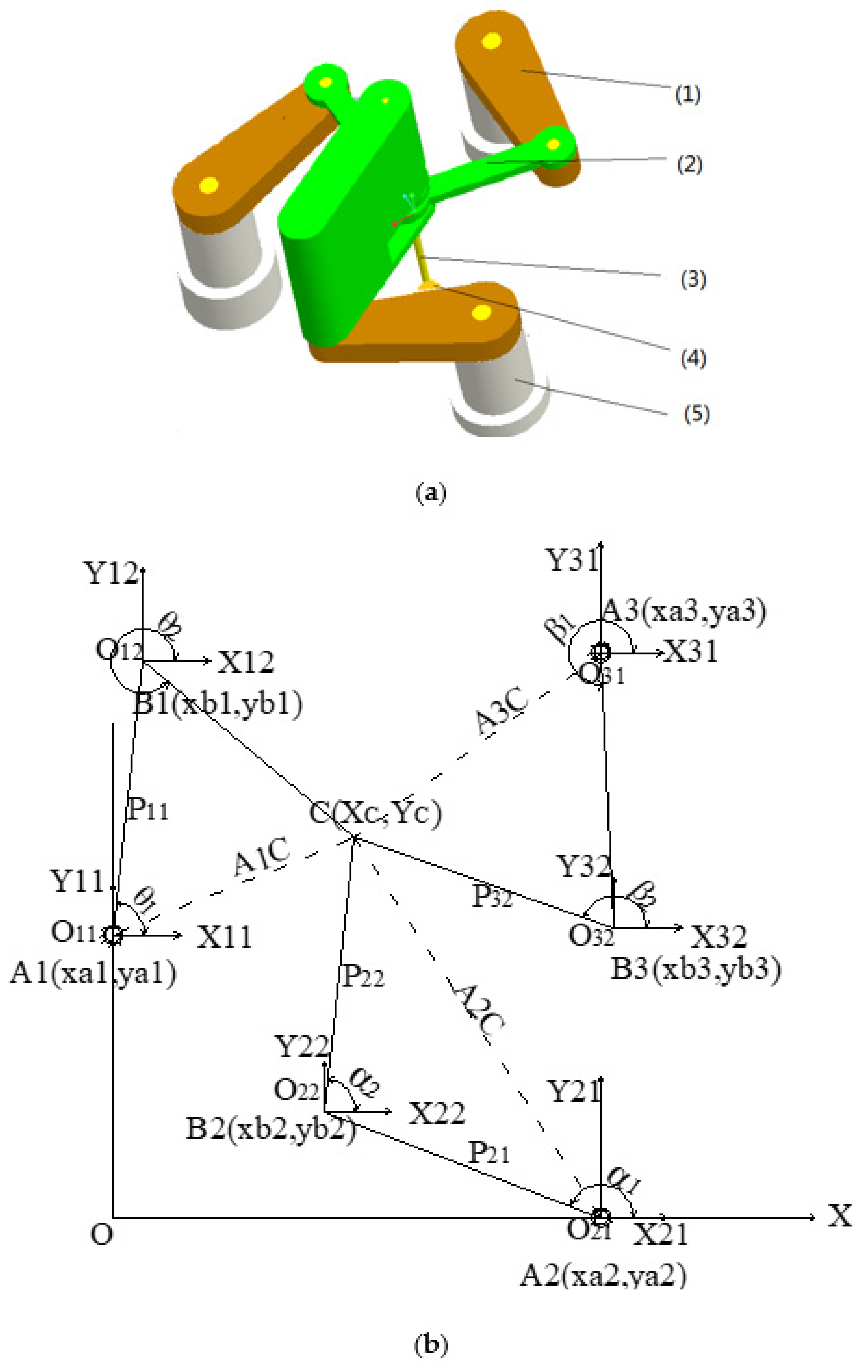
2. Establishment of Kinematics Equation of 4-DOF Redundant Parallel Robot

The 4-DOF redundant parallel robot is composed of three plinths (5), 3 driving arms (1), 3 driven arms (2), an end-effector (3), and a pneumatic claw (4). The driver and speed reducer are installed on the plinth, and the end-effector is composed of a 2-DOF mechanism. The whole mechanism has the characteristics of avoiding singularity, increasing rigidity, and improving performance. The end-effector consists of two joints and a terminal pneumatic claw. The first joint moves in the Z direction, and the second joint rotates around the Z-axis, as shown in Figure 1a.

For obtaining the trajectory equation of each joint in joint space in Figure 1a, the coordinate system as shown in Figure 1b is established. In Figure 1b, the base coordinate is xoy, and the coordinates of the joints are $x_i{o}_i{y}_i$(i = 1, 2, 3). Three plinths A1 (Xa1, Ya1), A2 (Xa2, Ya2), and A3 (Xa3, Ya3) are used to connect the 3 driving manipulators. The driving and driven angle is $q_1\left({\theta }_1,{\alpha }_1,{\beta }_1\right)$ and $q_2\left({\theta }_2,{\alpha }_2,{\beta }_2\right)$, respectively. The length of the 3 driving arms and the 3 driven arms is L. The end-effector is $C\left(X,Y\right)$. The distance $\mathrm{Aic}$ from the base to the end-effector is as follows:

$$\mathrm{Aic}=\sqrt{{\left(X_C-xai\right)}^2+{\left(Y_C-\mathrm{yai}\right)}^2},\mathrm{i}=1,2,3$$

(1)

Using geometry and the Law of Cosines, the driving angle$q_1$ can be denoted as follows:

$$q_1=\left[\arctan \left(\right(Y_C-\mathrm{yai})/(X_C-\mathrm{xai}\left)\right)+\arccos (\mathrm{Aic}/(2\mathrm{L}\left)\right)\right]180/\pi$$

(2)

The follower angle $q_2$ is as follows:

$$q_2=a\mathrm{rccos}\left(\right(X_C-\mathrm{xai}-\mathrm{Lcos}{q}_1)/\mathrm{L})$$

(3)

where the $q$, $q_1$, and $q_2$ represent each driving joint variable, driven joint variable, and each joint variable, respectively. The coordinate vector of the end-effector is $q_C={\left[\begin{array}{cc}{X}_C& Y_C\end{array}\right]}^T$. From the kinematic equation, the velocity of the end-effector output terminal point C can be expressed as follows:

$$\{\begin{array}{c}{\dot{X}}_C=-L\sin (q_1){\dot{q}}_1-L\sin (q_2){\dot{q}}_2\\ {\dot{Y}}_C=L\cos (q_1){\dot{q}}_1+L\cos (q_2){\dot{q}}_2\end{array}i=1,2,3$$

(4)

$${\dot{q}}_C=J\dot{q}$$

(5)

In Equation (5), $J$ is the velocity Jacobian Matrix, which maps the joint space onto the operating space. The generalized velocity of the end-effector is$V\left(t\right)={\left[\begin{array}{cc}{\dot{X}}_C& {\dot{Y}}_C\end{array}\right]}^T$. Acceleration is $a\left(t\right)={\left[\begin{array}{cc}{\ddot{X}}_C& {\ddot{Y}}_C\end{array}\right]}^T$. The acceleration rate is $u\left(t\right)={\left[\begin{array}{cc}{\stackrel{⃛}{X}}_C& {\stackrel{⃛}{Y}}_C\end{array}\right]}^T$. Then, we have the following:

$$V\left(t\right)=J\dot{q}\left(t\right)$$

(6)

$$a\left(t\right)=\dot{J}\dot{q}\left(t\right)+J\ddot{q}\left(t\right)$$

(7)

$$u\left(t\right)=\ddot{J}\dot{q}\left(t\right)+2\dot{J}\ddot{q}\left(t\right)+J\stackrel{⃛}{q}\left(t\right)$$

(8)

From Equations (1)–(8), we can see that the velocity, acceleration, and acceleration rate in the joint space and the operating space are all sine functions of time. They are obtained by integrating the acceleration rate curve in joint space several times. These sine functions can reduce the calculation and improve the stability of the system. The trajectory optimization equation of system joint space is constructed according to the motion requirement of joint space, the indices of time, and the stability of system operation.

3. Construction Principle of 12-Phase Sine Jerk Motion Profile

During the process from initial status to final status, the robot component has to go through several stages, such as acceleration, constant speed, and deceleration, which form a typical jerk curve. To prevent the jerk caused by acceleration and deceleration of the mechanism, the sine curve is used to describe the acceleration rate in the acceleration and deceleration phase in Reference [7]. The three-phase sine jerk motion profile, a previous method to the 12-phase sine jerk motion profile, is shown in Figure 2.

In Figure 2, $jerk\left(t\right)$, the function of the jerk curve to time, can be expressed as follows:

$$jerk\left(t\right)=\{\begin{array}{c}{j}^{peak}\sin \left[\frac{2\pi }{T_a}\left(t-t_0\right)\right]t_0\in \left[t_0,t_1\right]\\ 0t_1\in \left[t_1,t_2\right]\\ -j^{peak}\sin \left[\frac{2\pi }{T_a}\left(t-t_2\right)\right]t_2\in \left[t_2,t_3\right]\end{array}$$

According to Figure 2 and the $jerk\left(t\right)$ function, the three-phase sine jerk motion profile, though the machine can move smoothly, fails to move with the highest speed or efficiency, causing each part cannot reach the movement limit of all key quantities, which can result in low running efficiency. Therefore, for reducing the running time of the component, the method, adding the middle constant velocity section, is adopted to make the component reach the peak value quickly and then gradually reduce to zero. Meanwhile, to ensure the component is in the motion saturated state as long as possible and to reduce the jerk frequency, the acceleration rate of the three-phase sine jerk motion profile is revised to the 12-phase sine jerk motion profile, as shown in Figure 3.

As is shown in Figure 3a, the angular acceleration rate curve $\stackrel{⃛}{q}\left(t\right)$ of the 12-phase sine jerk motion profile is a piecewise function of constant $j^{peak}$ motion at each positive and negative peak of a continuous sine curve. The analytical expression can be described as follows:

$$\ddot{q}\left(t\right)=\{\begin{array}{c}{j}^{peak}\sin \left[\frac{\pi }{2T_1}{\tau }_{\mathrm{i}}\right]{\tau }_1\in \left[t_0,t_1\right],{\tau }_{10}\in \left[t_9,t_{10}\right]\\ j^{peak}{\tau }_2\in \left[t_1,t_2\right],{\tau }_{11}\in \left[t_{10},t_{11}\right]\\ j^{peak}\sin \left[\frac{\pi }{2T_1}\left(\frac{{\tau }_i}{T_1}+1\right)\right]{\tau }_3\in \left[t_2,t_3\right],{\tau }_{12}\in \left[t_{11},t_{12}\right]\\ -j^{peak}\sin \left[\frac{\pi }{2T_1}{\tau }_{\mathrm{i}}\right]{\tau }_4\in \left[t_3,t_4\right],{\tau }_7\in \left[t_6,t_7\right]\\ -j^{peak}{\tau }_5\in \left[t_4,t_5\right],{\tau }_8\in \left[t_7,t_8\right]\\ -j^{peak}\sin \left[\frac{\pi }{2T_1}\left(\frac{{\tau }_i}{T_1}+1\right)\right]{\tau }_6\in \left[t_5,t_6\right],{\tau }_9\in \left[t_8,t_9\right]\end{array}$$

Furthermore, the angular acceleration function $\ddot{q}\left(t\right)$, the angular velocity curve function $\dot{q}\left(t\right)$, and the angular displacement curve function $q\left(t\right)$ are derived as follows, respectively:

$$\ddot{q}\left(t\right)=\ddot{q}\left(t_i\right)+{{\displaystyle \int }}_{t_i}^t\stackrel{⃛}{q}\left(t\right)dt$$

(9)

$$\dot{q}\left(t\right)=\dot{q}\left(t_i\right)+{{\displaystyle \int }}_{t_i}^t\ddot{q}\left(t\right)dt$$

(10)

$$q\left(t\right)=q\left(t_i\right)+{{\displaystyle \int }}_{t_i}^t\dot{q}\left(t\right)dt$$

(11)

According to the time interval shown in Figure 3, the piecewise function of the angular velocity $\dot{q}\left(t\right)$ of the 12-phase sine jerk motion profile function in each time interval can be expressed as

Table 1. Piecewise function of the angular velocity, $\dot{q}\left(t\right)$, of phase 12-phase sine jerk motion profile.

Time Interval	$\dot{\mathit{q}}\left(\mathit{t}\right)$ of Phase 12-Phase Sine Jerk Motion Profile
${\tau }_1\in \left[t_0,t_1\right]$	$\frac{2j^{peak}{T}_1}{\pi }{\tau }_1-j^{peak}{\left(\frac{2T_1}{\pi }\right)}^2\sin \left(\frac{\pi }{2T_1}{\tau }_1\right)$
${\tau }_2\in \left[t_1,t_2\right]$	$V_1+\frac{2j^{peak}{T}_1}{\pi }{\tau }_2+\frac{1}{2}{j}^{peak}{\tau }_2{}^2 ,V_1=j^{peak}\left[\frac{2T_1{}^2}{\pi }-{\left(\frac{2T_1}{\pi }\right)}^2\right]$
${\tau }_3\in \left[t_2,t_3\right]$	$V_2+j^{peak}\left[\left(\frac{2T_1}{\pi }+T_2\right){\tau }_3\right]-j^{peak}{(\frac{2T_1}{\pi })}^2\cos \left(\frac{\pi }{2T_1}{\tau }_3\right),V_2=j^{peak}\left(\frac{2T_1{}^2}{\pi }+\frac{2T_1{T}_2}{\pi }+\frac{T_2{}^2}{2}\right)$
${\tau }_4\in \left[t_3,t_4\right]$	$V_3+\left(A^{peak}-\frac{2T_1}{\pi }{j}^{peak}\right){\tau }_4+j^{peak}{(\frac{2T_1}{\pi })}^2\sin \left(\frac{\pi }{2T_1}{\tau }_4\right),V_3=A^{peak}\left(T_1+\frac{T_2}{2}\right)$
${\tau }_5\in \left[t_4,t_5\right]$	$V_4+\left(A^{peak}-\frac{2T_1}{\pi }{j}^{peak}\right){\tau }_5-\frac{1}{2}{j}^{peak} {\tau }_5{}^2,V_4=A^{peak}\left(2T_1+\frac{T_2}{2}\right)+j^{peak}[{\left(\frac{2T_1}{\pi }\right)}^2-\frac{2T_1{}^2}{\pi }]$
${\tau }_6\in \left[t_5,t_6\right]$	$V_5+\frac{2j^{peak}{T}_1}{\pi }{\tau }_6+j^{peak}{(\frac{2T_1}{\pi })}^2\cos \left(\frac{\pi }{2T_1}{\tau }_6\right),V_5=A^{peak}\left(2T_1+\frac{3T_2}{2}\right)-j^{peak}\left(\frac{2T_1{}^2}{\pi }+\frac{2T_1{T}_2}{\pi }+\frac{T_2{}^2}{2}\right)$
${\tau }_7\in \left[t_6,t_7\right]$	$V_6-\frac{2j^{peak}{T}_1}{\pi }{\tau }_7+j^{peak}{\left(\frac{2T_1}{\pi }\right)}^2 \sin \left(\frac{\pi }{2T_1}{\tau }_7\right),V_6=V^{peak}$
${\tau }_8\in \left[t_7,t_8\right]$	$V_7+\frac{2j^{peak}{T}_1}{\pi }{\tau }_8+\frac{1}{2}{j}^{peak}{\tau }_8{}^2$,$V_7=V^{peak}-j^{peak}\left[\frac{2T_1{}^2}{\pi }-{\left(\frac{2T_1}{\pi }\right)}^2\right]$
${\tau }_9\in \left[t_9,t_{10}\right]$	$V_8-j^{peak}\left[\left(\frac{2T_1}{\pi }+T_2\right){\tau }_9\right]+j^{peak}{(\frac{2T_1}{\pi })}^2\cos \left(\frac{\pi }{2T_1}{\tau }_9\right),V_8=V^{peak}-j^{peak}\frac{2T_1{}^2}{\pi }+\frac{2T_1{T}_2}{\pi }+\frac{T_2{}^2}{2}$
${\tau }_{10}\in \left[t_9,t_{10}\right]$	$V_9-\left(A^{peak}-\frac{2T_1}{\pi }{j}^{peak}\right){\tau }_{10}-j^{peak}{(\frac{2T_1}{\pi })}^2\sin \left(\frac{\pi }{2T_1}{\tau }_{10}\right),V_9=V^{peak}-A^{peak}\left(T_1+\frac{T_2}{2}\right)$
${\tau }_{11}\in \left[t_{10},t_{11}\right]$	$V_{10}-\left(A^{peak}-\frac{2T_1}{\pi }{j}^{peak}\right){\tau }_{11}+\frac{1}{2}{j}^{peak} {\tau }_{11}{}^2,V_{10}=V^{peak}-A^{peak}\left(2T_1+\frac{T_2}{2}\right)$
${\tau }_{12}\in \left[t_{11},t_{12}\right]$	$V_{11}-\frac{2j^{peak}{T}_1}{\pi }{\tau }_{12}-j^{peak}{(\frac{2T_1}{\pi })}^2\cos \left(\frac{\pi }{2T_1}{\tau }_{12}\right),V_{11}=V^{peak}-A^{peak}\left(2T_1+\frac{3T_2}{2}\right)$ $+j^{peak}\left(\frac{2T_1{}^2}{\pi }+\frac{2T_1{T}_2}{\pi }+\frac{T_2{}^2}{2}\right)$

Note: $\stackrel{⃛}{q}\left(t\right)$ is triple-integrated to obtain the angular displacement $q\left(t\right)$ curve. Similarly, the angular acceleration function and the angular displacement function can be treated by Equations (9) and (11).

.

4. Total Mechanical Energy Consumption Model

According to the interval segment of the 12-phase sine jerk motion trajectory, considering the time of the robot in each interval, the maximum torque, and rotational speed, the energy consumption of the mechanism will be reflected. Therefore, to minimize energy consumption, the 12-phase sine jerk motion profile is optimized, and the interval time is determined accordingly, which provides the basis for the follow-up control of the system.

4.1. Establishment of Total Mechanical Energy Consumption Model

According to Figure 1, the potential energy of a 4-DOF redundant parallel robot is zero due to its planar motion, and the effect of friction in each joint is ignored. It is supposed that the energy of the system is converted to kinetic energy completely under ideal conditions.

The angular velocity of the driving arm is ${\dot{q}}_1\left(t\right)=\left\{{\dot{\theta }}_1\left(t\right),{\dot{\alpha }}_1\left(t\right),{\dot{\beta }}_1\left(t\right)\right\}$. The driven angular velocity is ${\dot{q}}_2\left(t\right)=\left\{{\dot{\theta }}_2\left(t\right),{\dot{\alpha }}_2\left(t\right),{\dot{\beta }}_2\left(t\right)\right\}$. The mechanical energy consumption $E\left(t\right)$ of the whole robot is as follows:

$$E\left(t\right)=K_{11}\left(t\right)+K_{12}\left(t\right)+K_{21}\left(t\right)+K_{22}\left(t\right)+K_{31}\left(t\right)+K_{32}\left(t\right)$$

(12)

In Equation (12), $K_{i1}$ is the mechanical energy consumption of the driving arm Aibi. $K_{i2}$ is the mechanical energy consumption of the driven arm BiC$\left(i=1,2,3\right)$.$K_{i1}$ and $K_{i2}$ correspond to the kinetic energies in the parallel robot.

Thus, the mechanical energy consumption of the drive shaft is:

$$K_{i1}=\frac{1}{2}{m}_{i1}{p}_{i1}^2{\dot{q}}_1^2\left(t\right), i=\left(1,2,3\right)$$

(13)

The mechanical energy consumption of the driven shaft is:

$$\begin{gathered} K_{i2}=\frac{1}{2}{m}_{i2}{V}_2^2=\frac{1}{2}{m}_{i2}{L}^2{\dot{q}}_1^2\left(t\right)+\frac{1}{2}{m}_{i2}{p}_{2i}^2\left({\dot{q}}_1^2\left(t\right)+{\dot{q}}_2^2\left(t\right)+2{\dot{q}}_1\left(t\right){\dot{q}}_2\left(t\right)\right) \\ +m_{i2}{Lp}_{i2}{\mathrm{Cos}q}_2\left(t\right)\left({\dot{q}}_1^2\left(t\right)+{\dot{q}}_1\left(t\right){\dot{q}}_2\left(t\right)\right) \\ i=\left(1,2,3\right) \end{gathered}$$

(14)

In Equation (13), $p_{i1}$ is the distance from the centroid of the driving shaft to the center of the base. In Equation (14), $p_{i2}$ is the distance from the center of mass of the driven shaft to the center of the joint, as shown in Figure 1b.

According to Equation (3), $q_2\left(t\right)$ is a function of $q_1\left(t\right)$. $q_1\left(t\right)$ is obtained by integration of ${\dot{q}}_1\left(t\right)$. The Equation (12) is substituted into the Equations (13) and (14), to obtain the total mechanical energy consumption function, $E\left(t\right)$, in joint space.

4.2. Time–Energy Optimal Solution

In order to find the minimum value of $E\left(t\right)$, the total mechanical energy consumption function, and to determine the time of each interval, $E\left(t\right)$ is taken as the objective function. The energy and the time of each interval are solved by subdivisional calculation method under the constraint of kinematics and dynamics equations, for achieving a comprehensive optimization. Therefore, according to Equation (10), the angular velocity expression $\dot{q}\left(t\right)$ of the robot driving arm is obtained. The rotational speed, $n$, of the driving arm input is found to be as follows:

$$n=\frac{60}{2\pi i}\dot{q}\left(t\right)$$

(15)

According to the principle of electromechanics0, the motor maximum output power is $P_{max}$, and the minimal speed is $n_{min}$. The transmission ratio between the motor is $i$, and the maximum working efficiency of the driving arm is $\eta$. Then, the maximum input torque, $M_{max}$, of the driving arm can be obtained:

$$M_{max}=\frac{9550P_{max}}{n_{min}}*i*\eta$$

(16)

Finally, the torque relationship between the driving torque and the joints on the arm is obtained by utilizing the Lagrange dynamic Equation (17) as follows:

$$M=D\left(q\left(t\right)\right)\ddot{q}+H\left(q\left(t\right)\right){\dot{q}}^2\left(t\right)+C\left(q\left(t\right)\right)Q$$

(17)

In Equation (17), $M$ is the joint input torque:$M={\left(\begin{array}{cc}{M}_{i1}& M_{i2}\end{array}\right)}^T$. $D\left(q\left(\mathrm{t}\right)\right)$ is an Inertial matrix. $H\left(q\left(t\right)\right)$ is the Centrifugal Force matrix. $C\left(q\left(t\right)\right)$ is the Coriolis Force matrix, where$\ddot{q}={\left(\begin{array}{cc}{\ddot{q}}_1& {\ddot{q}}_2\end{array}\right)}^T$, ${\dot{q}}^2={\left(\begin{array}{cc}{\dot{q}}_1^2& {\dot{q}}_2^2\end{array}\right)}^T$, $Q={\left(\begin{array}{cc}{\dot{q}}_1{\dot{q}}_2& 0\end{array}\right)}^T$.

According to the objective function $E\left(t\right)$, taking rapidity and stability as the constraint conditions, the solution model is established as follows:

Objective function: $\min E\left(t\right)$

Constraint condition:

$$\begin{array}{c}s.t.\end{array}\{\begin{array}{c}\begin{array}{c}{g}_1\left(X\right)=-T_1<0\\ g_2\left(X\right)=-T_2<0\end{array}\\ g_3\left(X\right)=-j^{peak}<0\\ \begin{array}{c}{g}_4\left(X\right)=M-M_{max}<0\\ g_5\left(X\right)=\dot{q}-V^{peak}<0 \\ \begin{array}{c}{g}_6\left(X\right)=\ddot{q}-A^{peak}<0\\ \begin{array}{c}{h}_1\left(X\right)=q\left(0\right)-q_0=0\\ h_2\left(X\right)=q\left(t_{12}\right)-q_0-q_{12}=0\end{array}\end{array}\end{array}\end{array}$$

In the equation, $q_0$ is the initial angle of the driving joint; $q_{12}$ is the endpoint angle of the driving joint. The variable is $X={\left(\begin{array}{cc}{T}_1& T_2\end{array}\right)}^T$. Moreover, $g_u\left(X\right)\left(u=1,2,\cdots ,6\right)$ is an inequality constraint, where $g_1\left(X\right), g_2\left(X\right),\mathrm{and} g_3\left(X\right)$ denote that the values of $T_1$,$T_2$, and $j^{peak}$ are greater than zero. Moreover, $g_4\left(X\right)$ is the torque constraint, $g_5\left(X\right)$ is the angular velocity constraint, and $g_6\left(X\right)$ is the angular acceleration constraint.

An equality constraint $h_z\left(X\right)\left(Z=1,2\right)$ is established from the starting and ending positions of the locus, where $h_1\left(X\right)$ represents the angular displacement starting angle of the 12-phase sine jerk motion profile, and $h_2\left(X\right)$ represents the angular displacement ending angle of the 12-phase sine jerk motion profile. The optimization variables is $T_1$, $T_2$, and $j^{peak}$. The optimization algorithm penalty function is used to optimize multiple variables of the objective function under constraints. According to the objective function, equality constraint condition, and inequality constraint condition, the penalty function $\varphi T_1,T_2,r^{\left(k\right)}$ is constructed as follows:

$$\varphi T_1,T_2,r^{\left(k\right)}=E\left(t\right)-r^{\left(k\right)}{\displaystyle \sum }_u^m\frac{1}{g_u\left(X\right)}+\frac{1}{r^{\left(k\right)}}{\displaystyle \sum }_{z=1}^p{\left[h_z\left(X\right)\right]}^2$$

(18)

In Equation (18), $r^{\left(k\right)}$ is the penalty factor, a decreasing sequence of positive numbers.

According to Equation (18), the parameters $T_1,T_2,$ and $j^{peak}$ in the motion trajectory are calculated, and the penalty function $\varphi T_1,T_2,r^{\left(k\right)}$ is minimized to obtain the optimal trajectory value.

5. Simulation and Experiment Results Analysis

To verify the correctness of the above theoretical analysis, Matlab was used in the simulation. Servo studio, GPM II, Mct 2008, Matlab, and other software were used in the experiment. Taking the 4-DOF redundant parallel robot shown in Figure 4a as the foundation of experiment and simulation analysis, the joints and coordinate positions are defined as shown in Figure 4b.

The structure and dynamic parameters of the robot in Figure 4b are shown in

Table 2. The structure and dynamic parameters of the 4-DOF parallel robot.

Parameter	Quality $\left(Kg\right)$	Length $\left(m\right)$	Distance from Center of Mass to Joint $\left(m\right)$	Moment of Inertia $\left(Kg\times m^2\right)$
1	2.1	0.2440	0.1096	0.0252
2	8.5	0.2440	0.0957	0.0778
3	2.1	0.2440	0.1096	0.0252
4	0.4	0.2440	0.1260	0.0064
5	2.1	0.2440	0.1096	0.0252
6	0.4	0.2440	0.1260	0.0064

.

In Figure 4a, the 4-DOF parallel robot adopts Tamogawa AC servo motor TS4603 N7185 E200 with rated speed $n_e=3000\mathrm{r}/\mathrm{m}\mathrm{i}\mathrm{n}$, max speed $n_{max}=5000\mathrm{r}/\mathrm{m}\mathrm{i}\mathrm{n}$, rated power $P_e=400w$, and reduction ratio i = 80. The number of pulses in the encoder per turn is $2^{17}$. The motion parameters, maximum allowable limits, of each joint in the joint space are shown in

Table 3. Results of kinematic parameter planning for each joint.

Joint Number Kinematic Parameter	Joint 1	Joint 3	Joint 5
Starting point $\left(\mathrm{deg}\right)$	60	177	−77
Starting point $\left(\mathrm{deg}\right)$	46	167	−54
Angular velocity limit value $\left(\mathrm{deg}/\mathrm{s}\right)$	25.913	17.074	42.574
Angular acceleration limit value $\left(\mathrm{deg}/{\mathrm{s}}^2\right)$	86.369	61.667	141.903
Jerk limit value $\left(\mathrm{deg}/{\mathrm{s}}^3\right)$	380.195	271.426	624.660

.

Then, the analysis object, the linear motion of the end effector from point A to point B in the operating space in Figure 1 and Figure 4b, is calculated by the mathematical software, using the 12-phase sine jerk motion profile function and penalty function equation. The obtained characteristic parameters and time segmentation values of the joint space are taken as the basis for the optimal trajectory simulation and experimental verification of the specific process, as follows.

5.1. Simulation Analysis of Stability and Accuracy of 12-Phase Sine Jerk Motion Profile

According to Table 1, an optimization algorithm is used to calculate the time $T_1=T_2=0.1\mathrm{s}$, and the total motion time is $T=8T_1+4T_2=1.2\mathrm{s}$, $j^{peak}=346.261\mathrm{d}\mathrm{e}\mathrm{g}/{\mathrm{s}}^3$. Combined with Figure 4, the three plinths of the parallel mechanism form an equilateral triangle, and the end-effector of the robot moves from point A to point B, just on the midline of the equilateral triangle. Thus, the kinematics curves of Joint 1 are equal to Joint 2, with Joint 3 equaling to Joint 6, and Joint 4 equaling to Joint 5. Based on the obtained curves of angular displacement, angular velocity, angular acceleration, and angular acceleration rate of a joint, the motion profile of each joint can be calculated by the relationship between the joint and other joints. Setting the rotation of the anticlockwise direction as the positive direction, the Joints 4 and 5 are in a positive direction, while Joints 1, 2, 3, and 6 are in a negative direction. The angular displacement, angular velocity, angular acceleration, and rate of change of angular acceleration of each joint are shown in Figure 5.

According to Figure 5, the above curves of each joint of the 4-DOF parallel robot have no abrupt changes during the operation of the mechanism, which shows that the whole process of the mechanism runs smoothly. There is a little transient jerk, a little periodic or aperiodic oscillation phenomenon. When the robot moves from the initial position to the terminal position, the curves are continuous from zero, within the allowable limit of the mechanism joints, ensuring sufficient precision and smoothness of the optimal trajectory. The peak value of each movement is very close to the limit value of constraint so that the operating efficiency of the machine can be fully reflected. To make the above process more intuitive, the key parameters are presented in

Table 4. Simulation result of joint motion parameters.

Joint Number	Joint 1	Joint 3	Joint 5
Kinematic parameter
Starting point $\left(\mathrm{deg}\right)$	60	177	−77
Stopping point $\left(\mathrm{deg}\right)$	46	167	−54
Ultimate angular velocity $\left(\mathrm{deg}/\mathrm{s}\right)$	23.600	16.850	51.204
Ultimate angular acceleration $\left(\mathrm{deg}/{\mathrm{s}}^2\right)$	78.660	56.163	129.238
Ultimate jerk $\left(\mathrm{deg}/{\mathrm{s}}^3\right)$	346.261	247.200	568.907

.

Compared with Table 3 and Table 4, the coincidence degree of the position of a starting point and endpoint between the initial set value and simulation result is 100%. The coincidence degree of the peak value of the limit angular velocity, the limit angular acceleration, the limit angular acceleration rate, and the maximum allowable limit value in each joint are all 91.050%. In theory, it is proved that the 12-phase sine jerk motion profile can meet the requirements of stability and accuracy of joint space trajectory of the 4-DOF parallel robot.

5.2. Comparative Analysis of Characteristic Parameters of 12-Phase, 3-Phase, and 15-Phase Sine Jerk Motion Profile

Experimentally, taking the three-phase and 15-phase sine jerk motion profile as the comparative basis to prove the superiority of the 12-phase sine jerk motion profile in trajectory planning, the experimental verification research is carried out around the characteristic parameters such as jerk amount, joint angular velocity, and joint energy consumption during a joint operation.

5.2.1. Comparison of Operational Stability

In the experimental platform shown in Figure 4a, the 3-phase, 12-phase, and 15-phase sine jerk motion profiles are sequentially input by offline programming in the robot motion program control language instruction, and the optimized time segments and $j^{peak}$ values are substituted.

For the straight-line trajectory from A to B in the operating space, it is set that the three-phase and 12-phase sine jerk motion profiles have the same starting and stopping point, and equaling motion time. In total, 101 sampling experimental data on Joint 1 were obtained. The experiment and simulation curves of each characteristic parameter on Joint 1 are drawn together, as shown in Figure 6, for showing the difference between simulation and experimental values of the robot under three-phase and 12-phase sine jerk motion profiles visually.

It can be seen from Figure 6 that the experimental and simulation curve of angular displacement are in good agreement under the three-phase or 12-phase sine jerk motion pro-file of Joint 1, which shows that the previous theoretical analysis is correct. The angular displacement of the 12-phase sine jerk motion profile is more smooth, which is a typical “S” type sine displacement curve. Compared with the angular dis-placement curve of the three-phase sine jerk motion profile, which is approximately a straight line, it can effectively alleviate the jerk during the operation of the mechanism and make the mechanism more flexible. Moreover, Figure 6b–d further shows that the angular velocity variation range, the magnitude of the joint’s torque, and the speed of the torque direction change of the robot joint are more conducive to the stable operation of the robot and more conducive to reducing the mutual jerk between the joints when running 12-phase sine jerk motion than the three-phase sine jerk motion during the operation of the robot.

For the curve trajectory from C to D in the operating space, it is set that the three-phase and 15-phase sine jerk motion profiles have the same starting and stopping point and equaling motion time. A total of 402 sampling experimental data on Joint 1 were obtained. The experiment and simulation curves of each characteristic parameter on Joint 1 are drawn together as shown in Figure 7 and Figure 8, for showing the difference between simulation and experimental values of the robot under 15-phase and 12-phase sine jerk motion profiles visually. Figure 7 shows the simulation experimental results of 12-phase sine jerk motion profile of Joint 1 as follows.

To use the filter to process the data with a certain delay, the delay in Figure 7b,c is not obvious, and the delay in Figure 7d is about 0.25 s. In the case of removing the effect of delay, it can be seen from Figure 7 that the experimental and simulation curve of angular displacement are in agreement under the 12-phase sine jerk motion profile of Joint 1, which shows that the previous theoretical analysis is correct.

Figure 8 shows the simulation experimental results of 15-phase sine jerk motion profile of Joint 1 as follows.

Figure 8 shows that the experimental and simulation curve of angular displacement is in a bad agreement under the 15-phase sine jerk motion profile of Joint 1. In the initial stage of the movement, the error between the actual position curve and the planned trajectory is small, and then the error gradually increases. Finally, the actual position curve has two sudden changes. The reasons for this phenomenon are as follows. The 4-DOF redundant parallel robot has a small working space. It means shorter trajectory movement, acceleration, and velocity peaks are both constrained by displacement, and there is no need for a constant acceleration phase or a constant velocity phase in the trajectory. The 15-phase sine jerk motion profile contains a constant acceleration phase and a constant speed phase. Therefore, in a small working space, the 12-phase sine jerk motion profile is more applicable than the 15-phase curve. Therefore, it shows that the 15-phase sine jerk motion profile is not fit for the small operation motion.

5.2.2. Comparison of the Amount of Jerk on Each Joint

To further quantify the above analysis process and expand the jerk on each joint, based on the experimental data and the method given in Reference [26], assume that the angular displacement, angular velocity, angular acceleration, and angular acceleration rate of the joint are all restricted. The jerk on the whole moving process is measured by the integral of the square of the $jerk\left(t\right)$ function, and then the calculation formula of the amount of jerk I of each joint is obtained as follows:

$$I={{\displaystyle \int }}_0^t{\left(jerk\left(t\right)\right)}^{2}dt$$

(19)

According to Equation (19), the jerk capacity of each joint is calculated as shown in

Table 5. Comparison of the peak jerk of each joints’ 3-phase and 12-phase.

Jerk Capacity of Each Joint	3-Phase Sine Jerk Motion Profile	12-Phase Sine Jerk Motion Profile
Joint 1	14,229	29.2180
Joint 3	72.539	14.8953
Joint 5	38,409.778	78.8711

Note: 12-phase sine jerk motion profile in the experiment.

when running on the three-phase and 12-phase sine jerk motion profile respectively:

The data in Table 5 directly show that the jerk of each joint, especially Joint 1, Joint 2, Joint 4, and Joint 5, decrease greatly, the jerk of the 12-phase sine jerk motion profile is greatly smaller than the three-phase sine jerk motion profile, and the force on each joint is more uniform. It proves, when the abovementioned 12-phase sine jerk motion profile is used, that the robot acceleration and deceleration process is more stable, with a better stability conclusion (lower jerk means more stable).

5.2.3. Speed Comparison

In order to respectively verify the rapidity of three-phase and 12-phase sine jerk motion profiles, under the process of end-effector motion, the peak angular velocity of each joint was obtained for quantitative comparison. The peak angular velocity of each joint is shown in

Table 6. Comparison of average peak angular velocity of joints’ 3-phase and 12-phase sine jerk motion profile in the experiment.

Angular Velocity of Each Joint (deg/s)	3-Phase Sine Jerk Motion Profile	12-Phase Sine Jerk Motion Profile
Joint 1	−17.409	−25.0653
Joint 3	−12.487	−18.3629
Joint 5	28.760	42.2544

.

When comparing the peak angular velocity of each joint under the three-phase and 12-phase sine jerk motion profiles in Table 6, we see that the peak value of the angular velocity of the 12-phase sine jerk curve is 34.86% higher than the three-phase sine jerk curve. The robot can move at a higher speed by the 12-phase sine jerk motion profile, and each joint can fully reach the operation limit of key parameters. Moreover, compared with the limit angular velocity of each joint in Table 2, the 12-phase sine jerk motion profile can accelerate each joint to a higher speed; that is, each joint is closer to the limit of motion, so the operation efficiency is higher.

5.2.4. Comparison of Energy Consumption

The energy consumption is taken as the optimization objective in the trajectory optimization of the 12-phase sine jerk function curve. The energy consumption of the whole process is measured by the integral of torque square, according to the driving torque function $M\left(t\right)$ in Lagrange dynamic Equation (20), combining with the calculation method of point-to-point track energy optimization in Reference [27]. The relationship between the energy consumption function $P$ and the moment$M\left(t\right)$ is as follows:

$$P={{\displaystyle \int }}_0^t{\left(M\left(t\right)\right)}^{2}dt$$

(20)

According to Equation (20), the energy consumption of each joint of the three-phase and 12-phase sine jerk motion profile is calculated as shown in

Table 7. Comparison of energy consumption of joints’ 3-phase and 12-phase sine jerk motion profile in the experiment.

Energy Consumption of Each Joint $\left(J\right)$	3-Phase Sine Jerk Motion Profile	12-Phase Sine Jerk Motion Profile
Joint 1	19.6823	29.5219
Joint 3	14.0532	21.0786
Joint 5	32.3380	48.5045

.

According to Table 7, the total energy consumption of each joint of the 12-phase sine jerk motion profile is increased by 66.67% compared with that of the three-phase sine jerk motion profile. However, compared with Table 4 and Table 5, the energy consumption of the 12-phase sine jerk motion profile can effectively reduce the transient jerk on each joint and improve the operation efficiency of each joint. Therefore, from the comprehensive comparison of operation accuracy, stability, and rapidity, the 12-phase sine jerk motion profile has more advantages and engineering application value.

6. Conclusions

To sum up, the high-speed motion trajectory optimized planning of the 4-DOF parallel robot was studied in this paper. By comparing the key characteristic parameters of three-phase and 12-phase sine jerk curves in simulation and experiment, the following conclusions are obtained:

(1)

When the joint space of the robot runs the 12-phase sine jerk motion profile, the overall operation is accurate and stable, and no sudden change of force and velocity exists in each joint, so the oscillation phenomenon is avoided.

(2)

Compared with the three-phase sine jerk curve, when the robot operates the 12-phase sine jerk motion profile, the force of each joint is more uniform, and the movement amount is closer to the maximum allowable limit value, so the operation efficiency is higher.

(3)

The energy consumption of the 12-phase sine jerk motion profile is higher than that of the three-phase sine jerk motion profile, but the former is far better than the latter in the stress uniformity and operation efficiency of each joint, which makes up for the defect of high energy consumption. As a result, the 12-phase sine jerk motion profile is still better than the three-phase sine jerk motion profile on the whole.

(4)

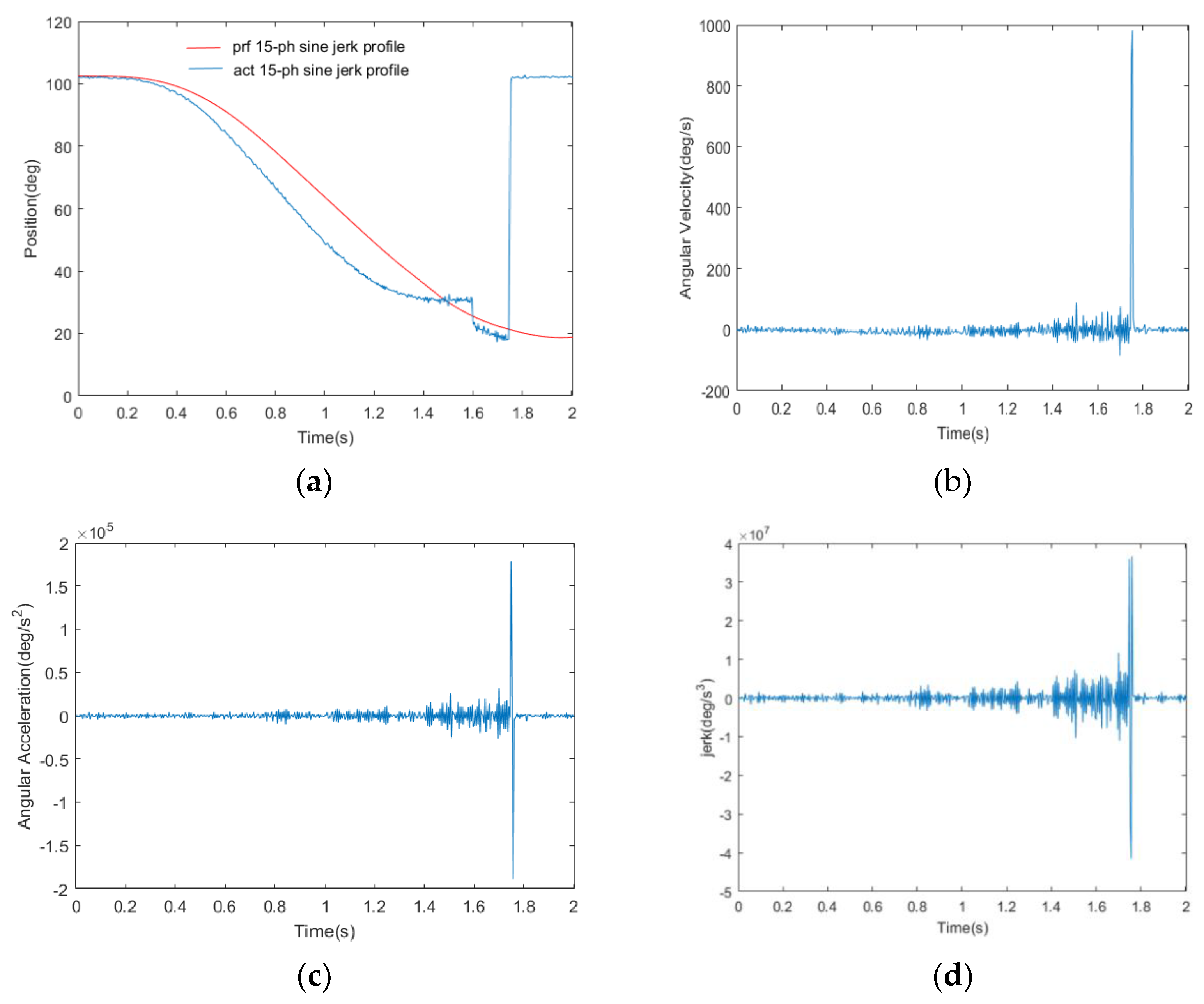
The 15-phase sine jerk motion profile is not suitable for trajectory planning in a small working space.

In future research, I will establish a dynamic equation closer to the motion model that includes friction force, based on the planned 12-phase sine impact motion profile. Then, I will design a controller to improve the accuracy of robot motion from the control level.

References

1. Pu, Y.S.; Shi, Y.Y.; Lin, X.J.; Guo, J. Attitude interpolation of industrial robot Hermite spline based on Logarithmic Quaternion. J. Northwestern Polytech. Univ. 2019, 37, 1165–1173. [Google Scholar] [CrossRef]
2. Abu-Dakka, F.J.; Assad, I.F.; Alkhdour, R.M. Statistical evaluation of an evolutionary algorithm for minimum time trajectory planning problem for industrial robots. Int. J. Adv. Manuf. Technol. 2017, 89, 389–406. [Google Scholar] [CrossRef]
3. Peng, J.W.; Liu, Y.; Zhao, Z.; Lou, Y.J. Joint trajectory planning for industrial robots with continuous acceleration. System Simulation Committee of CAS, Simulation Technology Application Committee of CAS, University of Science and Technology of China. In Proceedings of the 20th Chinese annual Conference on System Simulation Technology and its Applications (20th CCSSTA 2019), Nanchang, China, 3–6 August 2019; pp. 442–449. [Google Scholar]
4. Huang, Z. Study on mechanisms basic theory of parallel robot. Robot Tech. Appl. 2010, 11–14. [Google Scholar] [CrossRef]
5. Aquino, G.; Rubio, J.D.J.; Pacheco, J.; Gutierrez, G.J.; Ochoa, G.; Balcazar, R.; Cruz, D.R.; Garcia, E.; Novoa, J.F.; Zacarias, A. Novel Nonlinear Hypothesis for the Delta Parallel Robot Modeling. IEEE Access 2020, 8, 46324–46334. [Google Scholar] [CrossRef]
6. Rubio, D.J.J. SOFMLS: Online Self-Organizing Fuzzy Modified Least-Squares Network. IEEE Trans. Fuzzy Syst. 2009, 17, 1296–1309. [Google Scholar] [CrossRef]
7. Lu, Z. Principle and Application of Redundant Dof Robot; China Machine Press: Beijing, China, 2007. [Google Scholar]
8. Kim, J.; Croft, E.A. Online near time-optimal trajectory planning for industrial robots. Robot. Comput. Integr. Manuf. 2019, 58, 158–171. [Google Scholar] [CrossRef]
9. Li, H.Z.; Gong, Z.M.; Lin, W.; Lippa, T. Motion profile planning for reduced jerk and vibration residuals. Simtech Tech. Rep. 2007, 8, 32–37. [Google Scholar]
10. Fang, Y.; Qi, J.; Hu, J.; Wang, W.; Peng, Y. An approach for jerk-continuous trajectory generation of robotic manipulators with kinematical constraints. Mech. Mach. Theory 2020, 153, 103957. [Google Scholar] [CrossRef]
11. Valente, A.; Baraldo, S.E. Carpanzano Smooth trajectory generation for industrial robots performing high precision assembly processes Cirp Ann. Manuf. Technol. 2017, 66, 17–20. [Google Scholar] [CrossRef]
12. Wang, Y.; Yang, D.; Gai, R.; Wang, S. Sun Design of trigonometric velocity scheduling algorithm based on pre-interpolation and look-ahead interpolation. Int. J. Mach. Tools Manuf. 2015, 96, 94–105. [Google Scholar] [CrossRef]
13. Ruiz, G.A.; Fontes, J.V.C.; da Silva, M.M. The Influence of Kinematic Redundancies in the Energy Efficiency of Planar Parallel Manipulators. In Proceedings of the ASME 2015 International Mechanical Engineering Congress and Exposition, Houston, TX, USA, 13–19 November 2015; Volume 4A. [Google Scholar]
14. Paes, K.; Dewulf, W.; Elst, K.V.; Kellens, K.; Slaets, P. Energy Efficient Trajectories for an Industrial ABB Robot. Procedia Cirp 2014, 15, 105–110. [Google Scholar] [CrossRef] [Green Version]
15. Ho, P.M.; Uchiyama, N.; Sano, S.; Honda, Y.; Kato, A.; Yonezawa, T. Simple motion trajectory generation for energy saving of industrial machines. J. Control Meas. Syst. Integr. 2014, 7, 29–34. [Google Scholar] [CrossRef] [Green Version]
16. Carabin, G.; Scalera, L. On the Trajectory Planning for Energy Efficiency in Industrial Robotic Systems. Robotics 2020, 9, 89. [Google Scholar] [CrossRef]
17. Gadaleta, M.; Pellicciari, M.; Berselli, G. Optimization of the energy consumption of industrial robots for automatic code generation. Robot. Comput. Integr. Manuf. 2019, 57, 452–464. [Google Scholar] [CrossRef]
18. Xu, H.L.; Xie, X.R.; Zhuang, J.; An, S.W. Optimal time and energy trajectory planning for industrial robots. Chin. J. Mech. Eng. 2010, 46, 19–25. [Google Scholar] [CrossRef]
19. Gasparetto, A.; Zanotto, V. Optimal trajectory planning for industrial robots. Adv. Eng. Softw. 2010, 41, 548–556. [Google Scholar] [CrossRef]
20. Kazem, B.I.; Mahdi, A.I.; Oudah, A.T. Motion planning for a robot arm by using genetic algorithm. Jordan J. Mech. Ind. Eng. 2008, 2, 131–136. [Google Scholar]
21. Perumaal, S.; Jawahar, N. Synchronized trigonometric S-curve trajectory for jerk-bounded time-optimal pick and place operation. Int. J. Robot. Autom. 2012, 27, 385–395. [Google Scholar]
22. Zhang, S.; Cao, Y.; Sun, H. Application of Jacobian Matrix and determinant in robot motion. J. Beijing Inst. Technol. 2020, 40, 576–580. [Google Scholar]
23. Field, G.; Stepanenko, Y. Iterative dynamic programming: An approach to minimum energy trajectory planning for robotic manipulators. In Proceedings of the IEEE International Conference on Robotics and Automation, Minneapolis, MN, USA, 22–28 April 1996. [Google Scholar]
24. Bailon, W.P.; Cardiel, E.B.; Campos, I.J.; Paz, A.R. Mechanical energy optimization in trajectory planning for six DOF robot manipulators based on eighth-degree polynomial functions and a genetic algorithm. In Proceedings of the 2010 7th International Conference on Electrical Engineering Computing Science and Automatic Control, Chiapas, Mexico, 8–10 September 2010; pp. 446–451. [Google Scholar] [CrossRef]
25. Yang, Y.; Pan, S.F. Dynamics Analysis of 3-DOF Industrial Robots. Manuf. Autom. 2008, 40, 51–53. [Google Scholar]
26. Kyriakopoulos, K.J.; Saridis, G.N. Minimum jerk path generation. In Proceedings of the 1988 IEEE International Conference on Robotics and Automation, Philadelphia, PA, USA, 24–29 April 1988; pp. 364–369. [Google Scholar]
27. Martin, B.J.; Bobrow, J.E. Minimum-effort motions for open chain manipulators with task-dependent end-effector constraints. Int. J. Robot. Res. 1999, 18, 213–224. [Google Scholar] [CrossRef]
Figure 1. The structure of 4-DOF redundant parallel robot and the establishment of its coordinates system: (a) structure of robot, (1) driving arms, (2) driven arms, (3) end-effector, (4) pneumatic claw, and (5) plinth; (b) establishment of coordinates system.
Actuators 10 00080 g001
Figure 2. Three-phase sine jerk motion profile: (a) angular acceleration rate–time curve, (b) angular acceleration–time curve, (c) angular velocity–time curve, and (d) angular displacement–time curve. T a acceleration section, T v constant speed section, T a deceleration section.
Actuators 10 00080 g002
Figure 3. 12-phase sine jerk motion profile: (a) angular acceleration rate−time curve, (b) angular acceleration−time curve; (c) angular velocity−time curve, and (d) angular displacement−time curve.
Actuators 10 00080 g003
Figure 4. Experimental platform diagram of 4-DOF redundant parallel robot: (a) experimental platform and (b) top view of robot arm.
Actuators 10 00080 g004
Figure 5. Curves of angular displacement, angular velocity, angular acceleration, and angular acceleration rate of each joint: (a) angular displacement curve of each joint, (b) angular velocity curve of each joint, (c) angular acceleration curve of each joint, and (d) angular acceleration rate of each joint.
Actuators 10 00080 g005aActuators 10 00080 g005b
Figure 6. Simulation and experimental comparison curves of key characteristic in Joint 1: (a) angular displacement curve, (b) angular velocity curve, (c) angular acceleration curve, and (d) angular acceleration rate.
Actuators 10 00080 g006
Figure 7. Simulation and experimental comparison curves of 12−phase sine jerk motion profile key characteristic in Joint 1: (a) angular displacement curve, (b) angular velocity curve, (c) angular acceleration curve, and (d) angular acceleration rate.
Actuators 10 00080 g007
Figure 8. Simulation and experimental comparison curves of 15-phase sine jerk motion profile key characteristic in Joint 1: (a) angular displacement curve, (b) angular velocity curve, (c) angular acceleration curve, and (d) angular acceleration rate.
Actuators 10 00080 g008