Photogrammetric Measurement and Analysis of the Shape Profile of Pneumatic Artificial Muscles

Abstract

Inaccuracies in modeling of the geometric shape of PAMs has long been cited as a probable source of error in modeling and design efforts. The geometric shape and volume of PAMs is commonly approximated using a cylindrical shape profile, even though its shape is non-cylindrical. Correction factors—based on qualitative observations of the PAM’s general shape—are often implemented to compensate for error in this cylindrical shape approximation. However, there is little evidence or consensus on the accuracy and form of these correction factors. Approximations of the shape profile are also used to calculate the internal volume of PAMs, as experimental measurements of the internal volume require intrusive testing methods and specialized equipment. This research presents a photogrammetric method for measuring the shape profile and internal volume of PAMs. A test setup, method of image data acquisition, and a preliminary analysis of the image data, is presented in this research. A 22.2 mm (7/8 in) diameter PAM is used to demonstrate the photogrammetric procedure and test its accuracy. Analysis of the tested PAM characterizes trends of the shape profile with respect to pressure and contraction. The common method of estimating the diameter—through the use of the cylindrical approximation and initial geometry of the PAM—is tested by comparison to the measured shape profile data. Finally, a simple method of calculating the internal volume using the measured shape profile data is developed. The presented method of acquiring photogrammetric measurements of PAM shape produces an accurate characterization of its shape profile, thereby mitigating uncertainty in PAM shape in analysis and other efforts.

1. Introduction

Pneumatic Artificial Muscles (PAMs) are a form of soft actuator that is applied to an expanding number of applications for their unique characteristics such as their low weight and simple construction, inherent compliance, and high specific force and specific work capabilities. In a design environment where optimization techniques are increasingly used for mechanism development and packaging, it is becoming more important than ever to have accurate model representations of device components, including actuators, to accomplish effective design outcomes. Actuator design requirements typically include force and stroke values, while common actuator design constraints include actuator size, energy efficiency, and storage requirements. Models have been developed which address each of these design constraints and requirements for PAMs, but many of those models lack the accuracy required for their use in a world of increasingly tight design spaces, and improvements to those models has remained stagnant for years.

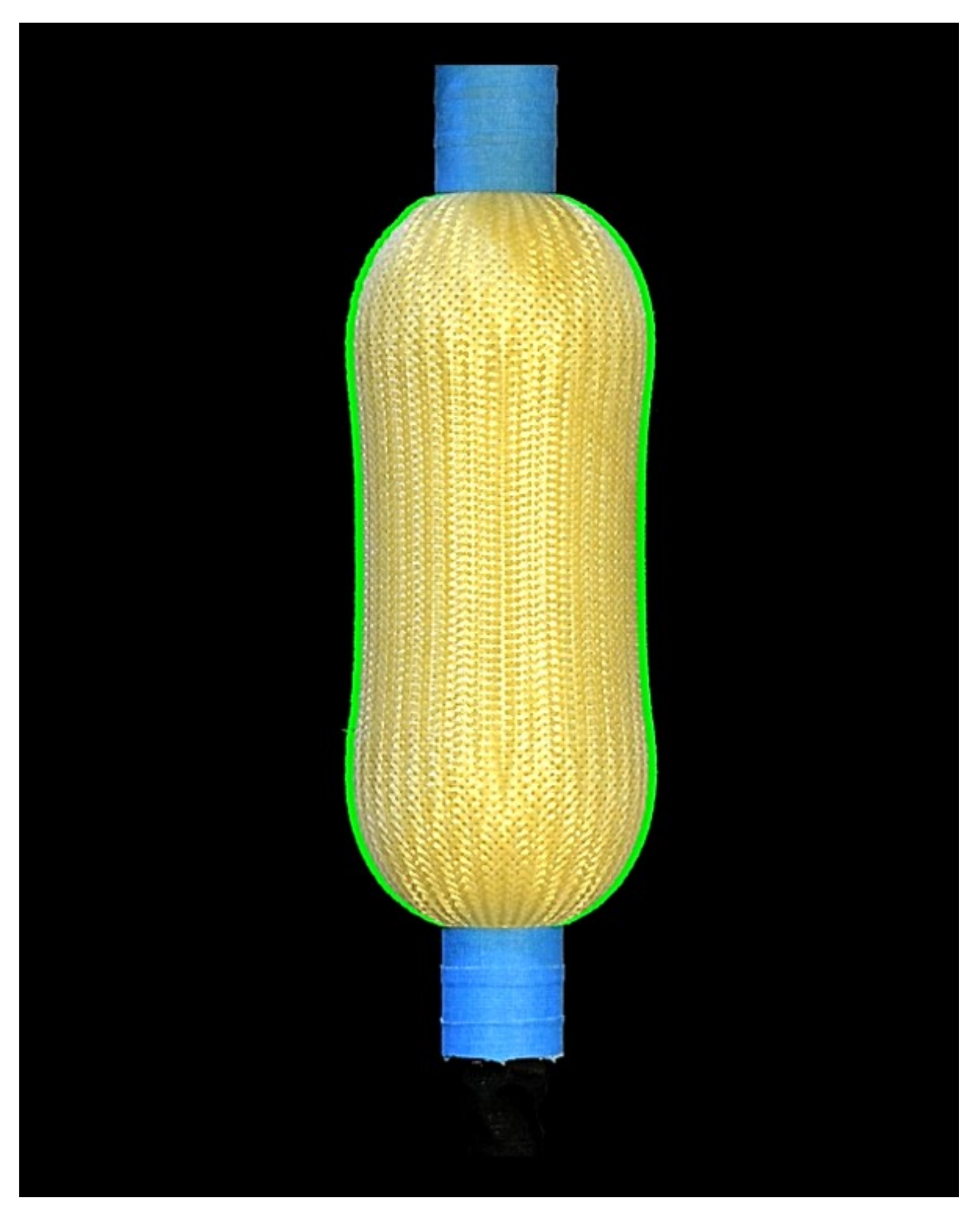
While continual improvements have been made in modeling the force response of PAMs, there has been little recent progress in the development of methods for characterizing the size and overall shape profile of PAMs during operation, parameters commonly used for calculating efficiency, fluid storage, and flow rate requirements. The PAM’s shape profile (Figure 1) has long been approximated through visual observations, and has often been cited as a suspected source of modeling error [1,2]. This paper seeks to remedy this by providing a new method of accurately measuring the PAM’s shape profile.

With the simple construction of an elastomeric bladder, a surrounding helically braided load-bearing sleeve, and rigid end-fittings at each end, a pressurized contractile PAM can provide a tensile force along its longitudinal axis. Upon internal pressurization of the PAM, the radial pressure force of the internal fluid is transferred through the bladder to the braided sleeve. The braided sleeve transforms that radial force into an axial force expressed at each end-fitting. The actuation force produced by a PAM is a function of its active length and internal pressure states. The actuation force is at a maximum at its resting length, when the braid angle, defined with respect to the radial axis of the PAM, is at a maximum. As the PAM contracts, the braid angle reduces and the bladder strain increases, resulting in a reduction of actuation force until the PAM reaches a pressure-dependent maximum free contraction in its zero-actuation-force state.

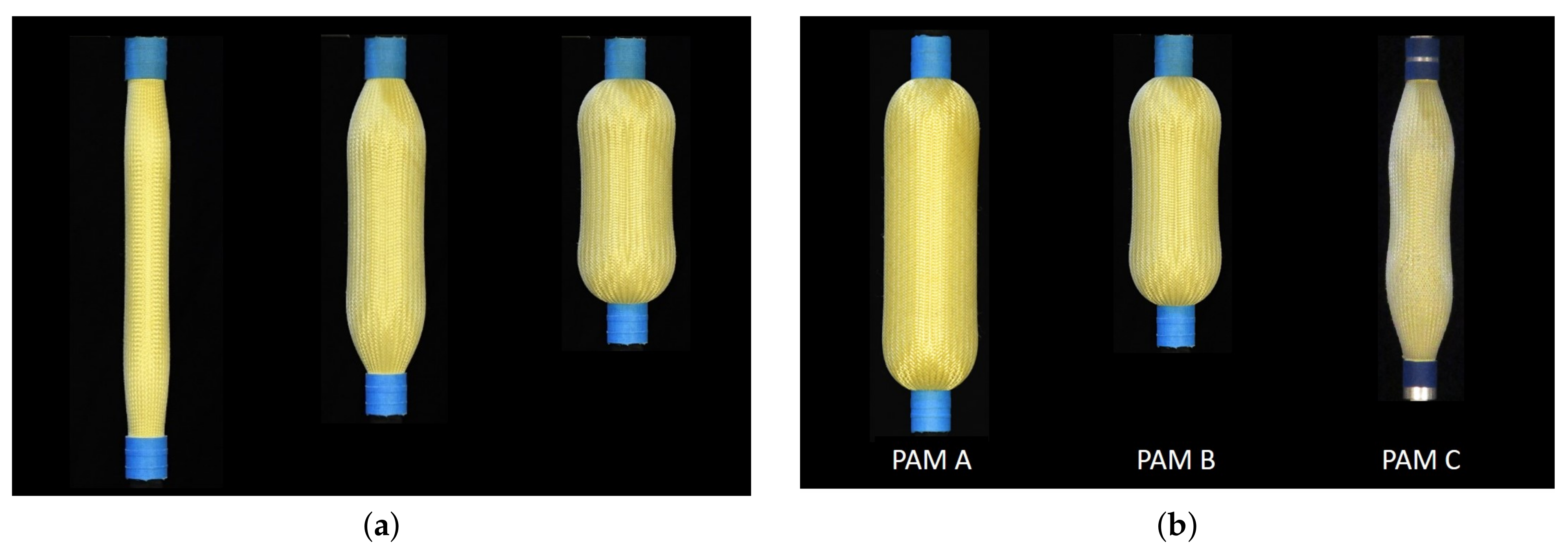
The shape profile of a PAM changes with contraction of its length (Figure 2a). At its resting length, the PAM has an apparent constant diameter and braid angle along its length. As a PAM contracts in length, its diameter expands and the braid angle reduces as a function of the position along the length of the PAM. The braid geometry is constrained only at each end-fitting where the diameter is equal to the initial diameter. 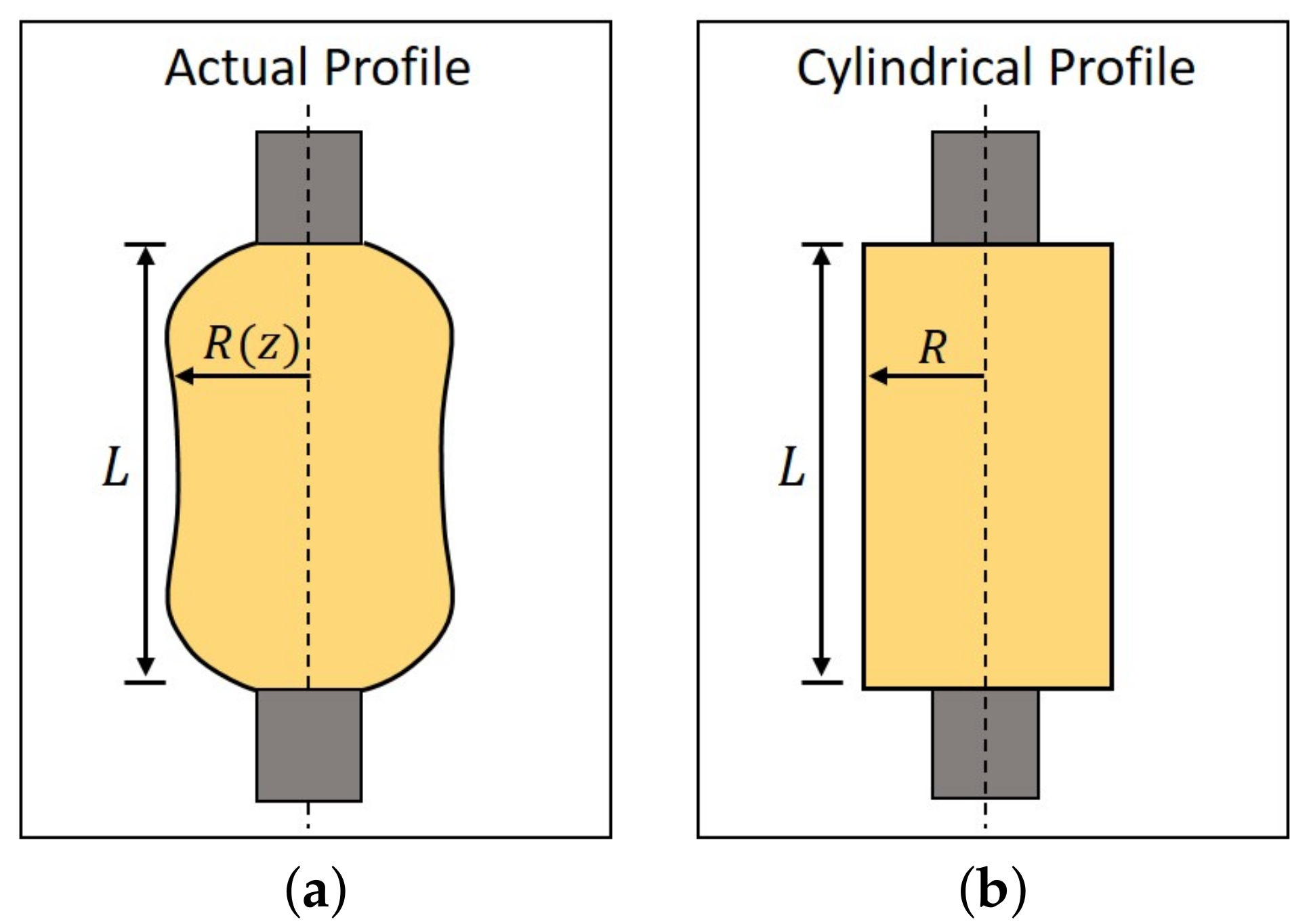The shape profile is also highly dependent on the PAM, with PAMs of identical material construction having visible differences in their shape profile (Figure 2b). PAMs have had shape profiles that range from a more cylindrical mid-section shape to ones that have constant variations in curvature along their entire length. The bulbous shape of a PAM is often approximated as a cylindrical profile with a constant diameter along its entire length (Figure 3). Assuming the braid is inextensible, the cylindrically approximated shape enables a simplification of analysis through the so-called triangle relationship that correlates the PAM’s diameter, braid angle, and active length. This cylindrical approximation serves as the basis for many existing PAM models, including models for volume and actuation efficiency, as well as for force-response models that have been developed using both force-balance [3] and principle of virtual work approaches [4].

Past modeling efforts of PAMs have often centered around rudimentary representations of their shape profile. While the cylindrical approximation of the shape profile simplifies analysis and modeling, it has often been cited as a suspected source of error, thus making it the subject of more detailed modeling efforts [1,2,5,6,7,8,9]. Many researchers have inferred that the reduction in diameter near each end-fitting produces what is often termed as end-effects that act to decrease the force response of the PAM. Modeling corrections that take end-effects into account for the principle of virtual-work models often attempt to serve to more accurately calculate the internal volume of the PAM. Correction efforts for the force-balance modeling method have centered around the effective reduction of active length due to the non-cylindrical shape profile. Tondu [7] was the first to use an end-effect correction factor by including a tuning parameter that effectively amplified the contraction ratio in the force response equation. Kothera et al. [1] took a similar approach by reducing the effective active length in the model by two-times the difference of the current and initial radius. Most models that have taken the shape profile of the PAM into account have maintained a cylindrical approximation for the PAM’s midsection, while applying shape corrections to the regions near the end-fittings at each end. Assumed shape profiles have included a stepped cylindrical approximation [8], a 90 deg circular arc [5,10], a semi-ellipsoid [6,9], a conic frustum [8], and the partial surface area of an elliptic toroid [2]. These shape profiles are often selected based on qualitative observations and ease of computation. Only Meller et al. [9] has noted that volume measurements appear to show that the cylindrical approximation may be sufficient for modeling the internal volume of the PAM.

Our experience with PAMs has found that the overall shape profile of a PAM is variable, and often exhibits undulating curvature along the full length of the PAM. Having a quantitative method of measuring the shape profile of PAMs would be highly beneficial for improving the accuracy of models that rely on PAM geometry.

Having a more accurate measurement of the shape profile would also aid in characterizing the PAM’s internal volume which is often used in defining an actuator’s system requirements such as the working fluid flow rate and storage volume requirements. First-cut estimations of internal volume are often made using the cylindrical approximation of the PAM, while end-effects corrections are sometimes included to account for the reduced volume near each end-fitting with unknown improvements to accuracy. Some researchers have turned to quantifying the internal volume through experimental approaches [9]. While experimental methods should provide accurate calculations of internal volume, they often require specialized test equipment. To date, experimental methods have required either submerging the PAM in water, or pressurizing the PAM using water from a closed graduated cylinder [9], and then tracking the change in water level as the PAM contracts in length. The specialized equipment required for characterizing the volume using these methods not only subject the PAM to fluid that its material composition may not be compatible with, but also requires adjustment, replacement, or even redesign of the test setup components depending on the size and length of the PAM to be tested. Conversely, an experimental method that can test PAMs of all sizes while not requiring specialized equipment is desirable.

It is evident that previous PAM research efforts have relied on multiple different assumed shape profiles without consensus on which ones best fit the observed profiles, and without any conclusive measurement of their accuracy. This paper seeks to provide an experimental method that enables quantitative analysis of the shape profile of PAMs for improved accuracy in modeling efforts. In this research, photogrammetry, the science of making dimensional measurements of physical objects from photographic images [11], is adapted for use in the measurement of the PAM’s shape profile. An overview of the photogrammetric methods applied in this research are presented first. A test setup for image acquisition is introduced followed by a method of image analysis to render the shape profile measurements from the acquired images. The photogrammetric methods are demonstrated through example by testing a 22.2 mm (7/8 in) diameter, 236 mm (9-9/32 in) long PAM. The results from testing the PAM are presented, followed by analysis of the PAM using the photogrammetric data. The obtained shape profile data is compared to the profiles assumed by the cylindrical approximation. The validity and accuracy of the cylindrical approximation is tested. If more detailed and accurate modeling forms are required, the development of a fit equation is presented for use that accurately replicates the curvature of the PAMs shape profile. Potential improvements to current modeling efforts are also presented, including a demonstration of how easily inaccurate initial geometric conditions can be applied to models without having photogrammetric data available to reference. The profile data is then used to present a simple and accurate method of characterizing the internal volume of PAMs. Finally, the ability of the photogrammetric test method to be universally adopted is demonstrated through shape profile characterizations of PAMs ranging in length from 236 mm to 508 mm, and diameters of 22.2 mm and 57.2 mm. Overall, this paper aims to provide a new method of characterizing PAMs that has the potential to enlighten future modeling efforts with findings that are not otherwise realizable, and with measurements that have not previously been quantifiable.

2. Test Methods

Development of the test setup and methods focused on simplicity to ensure that the photogrammetric characterization would require only an adaptation of current PAM test setups without the need for specialized equipment or photography expertise. The photogrammetric methods performed for this research are detailed in this section to provide context for the test procedure that follows.

2.1. Image Acquisition

There are multiple methods of photogrammetric image acquisition that are capable of achieving various levels of image scene reconstruction. Both the number of measurable dimensions of an imaged object, and the requirements for scaling the object in the imaged scene are dependent on the number of cameras used and their relative positioning (i.e., imaging configuration). Imaging configurations include single-, stereo-, and multi-image photogrammetry methods [12]. Stereo-image and multi-image methods provide three-dimensional scene reconstruction and require either the use of multiple cameras or the controlled movement of a single camera. Single-image photogrammetry requires just a single camera in a fixed position, but only provides a two-dimensional planar view of the imaged object. This shortcoming can be overcome, however, by enlisting additional prior knowledge of the imaged object. Three-dimensional measurements can be achieved with just a single camera if geometric relations, measurements, or symmetries of the object are linked to the image.

The scale of an object in an image must be known to acquire its photogrammetric measurements. Scale is defined as the ratio of the size of an object in the imaged world (i.e., in pixels) to its size in the physical world. The scale of an object in an image depends on five things: (a) the object’s distance and position with respect to the camera, (b) the lens used by the camera, (c) the distance of the lens from the image sensor plane, (d) optical distortion due to inherent imperfections in the lens, (e) perspective distortion (i.e., radial distortion) which is dependent on the angle-of-view of the object in the image [11]. These camera state values can be used for scaling the imaged object, but they can also be arduous and time consuming for the layman to obtain. A simpler method of scaling employs the placement of an object with known dimensions into the image scene to calibrate the scaling of the object. This can be achieved by placing a ruler adjacent to the object of interest in the image scene prior to testing, as is done in this research. It is important to note that measurement accuracy is highly dependent on the image resolution provided by the camera used for image acquisition, as well as the position of the camera with respect to the measured object.

2.2. Image Analysis

The goal of the photogrammetric analysis is to obtain the shape profile dimensions of the PAM’s braid from photogrammetric images such as the image in Figure 1. In order to do this, image analysis techniques must be applied to isolate the PAM’s braid within each photographed image. Image analysis techniques include locating object boundaries, or segmenting image pixels into groups, based on color information such as color values (e.g., brightness, hue, etc.). With potentially thousands of images to be analyzed, it is essential to have automated methods of identifying and outlining objects of interest within images. The image segmentation and object identification techniques used in this paper are outlined in the following sections.

2.2.1. Color Model

Segmentation of an image is the process of grouping the pixels of an image based on their color values. With color contrast between objects in an image, an image can be segmented and reduced to isolate pixels in an area of interest. With image segmentation based on the color component values of each pixel, an important first step is the decision of what color model to use.

A color model is the mathematical representation of a color as a tuple of numbers. The RGB color model is commonly used to define pixel color in photographic images, but is often problematic for use in image analysis. The RGB color space is not a perceptual color space which makes it difficult to perceive how changes in color components (R, G, and B) will alter the hue and brightness of the color. This makes it difficult and imprecise to define a range of R, G, or B based on color, hue, or brightness, that would enable a desired segmentation of an image [13]. Another difficulty that arises for image segmentation when using the RGB color model results because normalized RGB component values are not invariant with changes in lighting or shading [14]. This makes the RGB component values vary unpredictably with fluctuations in brightness across an object’s surface from shadows, specular reflections, or changes in illumination due to motion of an object.

A color model that is more suitable than RGB for use in image analysis is the hue, saturation, and value (HSV) color space. The HSV color space provides a more intuitive method of defining colors that is beneficial for performing image segmentation [14,15,16]. As illustrated in Figure 4 [13], the HSV color space can be represented as a cylindrical space with hue, saturation, and value represented along respective coordinate axes.

Hue is defined as a 0–360 degree value that correlates to an angular position within the cylinder, and represents a color’s position within the color spectrum. Hue is helpful in segmenting an image based on color in a way that is invariant to changes in lighting conditions. Saturation, represented as a 0–100% value along the radius of the cylindrical space, defines the vividness of a color’s hue. Desaturation of a color occurs with added white light. Value, which is represented as a 0–100% value along the height of the cylindrical space, defines the perceived brightness of a hue. Sometimes described as relative brightness, value can be used to describe a color in varying lighting conditions. Therefore, segmentation using the value color component can be used to segment objects within an image based on their relative brightness [17]. Although photographic image data is often defined using the RGB color space, it can be converted to the HSV color space by using the following equations [18]:

$$M=max(R,G,B)$$

(1)

$$m=min(R,G,B)$$

(2)

$$\begin{array}{cc}\hfill H& ={60}^{\circ }\ast \left\{\begin{array}{cc}undefined\hfill & \mathrm{if}M=m\hfill \\ \frac{G-B}{M-m}mod6\hfill & \mathrm{if}M=R\hfill \\ \frac{B-R}{M-m}+2\hfill & \mathrm{if}M=G\hfill \\ \frac{R-G}{M-m}+4\hfill & \mathrm{if}M=B\hfill \end{array}\right.\hfill \end{array}$$

(3)

$$\begin{array}{cc}\hfill S& =\left\{\begin{array}{cc}0\hfill & \mathrm{if},M=0\hfill \\ \frac{M-m}{M}\hfill & ,\mathrm{otherwise}\hfill \end{array}\right.\hfill \end{array}$$

(4)

$$\begin{array}{cc}\hfill V& =M\hfill \end{array}$$

(5)

An image can be segmented based on the hue, saturation, or value component of each pixel. The invariance of hue to lighting conditions makes it a good candidate for color-based image segmentation. Care must be taken, however, to avoid use of hue segmentation in areas where pixel colors are near the hue singularity condition. Hue singularity occurs with colors that have saturation and value levels near zero (i.e., grayscale colors). In this color region, imperceptible changes in color can produce large fluctuations in hue. Attempts at hue segmentation near the singularity condition will result in arbitrary and inaccurate segmentation [14]. Those regions are better suited for segmenting based on saturation or value. For this research, pixel colors are defined in the HSV color space to segment each image based on relative brightness (i.e., value) and hue.

2.2.2. Boundary Detection

Automated identification of objects within an image boils down to the practice of segmentation through boundary detection. Common methods of boundary detection include edge detection and thresholding. Edge detection methods identify boundaries of objects by locating the sharp changes in color or light intensity that are characteristic of object boundaries [17]. It is often performed using gradient-based methods such as Canny edge detection [19]. Thresholding techniques, on the other hand, segment an image by grouping image pixels by comparing their color value to a set threshold value. Since thresholding locates areas of an image and not edges, finding boundaries through thresholding requires an additional step of using a method of locating and tracing object boundaries.

Edge detection methods are effective at detecting edges with sharp contrast, but can have difficulty with random specular reflections, or with soft edges that have small color gradients [17]. Identification of the edge of the PAM braid using edge detection methods proved to be difficult due to the soft edges of the PAM’s bulbous shape, and random spikes in brightness due to specular reflections off the surface of the Kevlar braid. However, the ruler used for calibration, with its flat surface and high-contrast hatch markings, was found to be an ideal candidate for edge-detection methods, as detailed in the Test Methods-Image Analysis section.

Thresholding techniques, when combined with a boundary tracing algorithm, can serve as a more robust method of boundary detection for identification of the PAM’s braid. Setting a color threshold can be performed manually through subjective analysis, but automated methods of thresholding have been developed that can identify a suitable threshold in a consistent and time-efficient manner. Automated methods of thresholding are typically based on color histogram analysis. The histogram defines the distribution of the number of instances of each color value in an image. Setting a threshold divides the histogram into two classes (i.e., groups) with all pixels below the color value threshold grouped into one class, and all pixels above the color value belonging to a second class. An image is commonly transformed into a class-membership based binary image to provide a visual representation of the threshold segmentation, and to serve as an input in many boundary tracing algorithms. Otsu’s method is a common method of histogram-based thresholding that is used in this research [17,20,21]. This method’s algorithm recursively searches for a threshold value that can divide the histogram into classes that have a maximum inter-class variance.

The algorithm is detailed as follows. Let us consider a certain color value (e.g., H, S, or V) to set a threshold on. Each pixel of an image is represented by L color value levels of the histogram (e.g., 0–100% for S or V), and within the histogram, the height of each color value bar represents the fraction of the total number of pixels at each respective color value level. For a given threshold, the pixels are separated into two classes ($i=1,2$). $w_i$ is equal to the probability of a pixel being in class i, and ${\mu }_i$ and ${\mu }_T$ are the mean value of each class and the total, respectively. Otsu’s method then finds the optimal threshold value by maximizing the inter-class variance, ${\sigma }_b$, using the following Equation [20,21]:

$${\sigma }_b^2=w_1{({\mu }_1-{\mu }_T)}^2+w_2{({\mu }_2-{\mu }_T)}^2$$

(6)

Otsu’s method is utilized for image segmentation, with Figures 9b and 10b providing illustrations of the relative brightness and hue histograms, respectively, with thresholds placed using Otsu’s method.

With an area of interest identified through threshold segmentation, the boundary of the area must then be traced with a contiguous line. A simple method of boundary tracing used in this research is the Moore-Neighbor algorithm [22,23]. With a binary image as the input, the Moore-Neighbor tracing algorithm locates any clusters of pixels of the same class, and then traces their boundaries. Starting at a pixel along the boundary of a cluster, the recursive Moore-Neighbor algorithm steps along a boundary until it meets a defined end condition.

The basis of the Moore-Neighbor algorithm is the Moore-Neighborhood of a pixel. A pixel’s Moore-Neighborhood (Figure 5a) is the set of eight pixels that surround a pixel of interest (pixel C). To advance along a boundary, the algorithm examines the Moore-Neighborhood of a boundary pixel in the clockwise direction, starting from the previously found boundary pixel (pixel P), until it comes upon the next boundary pixel. This process continues recursively until a stopping condition is met. A frequently used stopping condition is the Jacob’s stopping criterion. This criterion states that the Moore-Neighbor algorithm shall stop after visiting the start pixel at least twice, or after entering the start pixel from the same direction as it was initially entered.

Figure 5b provides an example of Moore-Neighbor tracing. A cluster of pixels of the same class (gray) is identified, and a start boundary pixel (pixel 1) located at the boundary of the cluster is established. From pixel 1, the Moore-Neighborhood search begins until the next boundary pixel (pixel 2) is reached. The algorithm repeats until it arrives back at the start boundary pixel from the original direction. The overall boundary traced for this cluster is identified as pixels 1–8.

Through the detection of the boundary of an area of interest (e.g., the braid) within an image realized, analysis of the size and shape of the boundary can then commence as desired.

3. Procedure

The methods of image acquisition and analysis described in the previous section are employed by this research, as detailed in this section. Photogrammetric data is acquired and the image is then reduced down to a traced outline of the PAM braid for further analysis of the shape profile.

Photogrammetric data of the shape profile is acquired while simultaneously characterizing the isobaric force-contraction response of the PAM. Testing of the force response is performed using the same methods as done in past PAM research [5,24]. The PAM is mounted in a MTS servo-hydraulic test machine, and is quasi-statically stroked between its minimum and maximum contraction length states while maintaining a constant internal working fluid pressure. The MTS machine directs a controlled stroking motion of the PAM while recording external inputs of pressure (Omega PC209-200G5V), and force (Honeywell Model 31 Mid 1000 lbf load cell), which provides a complete data set to characterize the isobaric force-contraction response of the PAM. The PAM is mounted in the MTS machine at each end through clamped fixtures (Figure 6). The top fixture serves as both a mounting point for the pressure sensor and as a conduit for air to travel into and out of the PAM. The bottom fixture connects to the load cell that is mounted inline with the PAM.

3.1. Image Acquisition

For simplicity of implementation, image acquisition is performed with the single-image photogrammetry configuration. The test setup to perform the force response and shape profile characterization is shown in Figure 7. Photogrammetric data acquisition requires the addition of only a camera, a backdrop, lighting, and masking of components. A camera is placed in a fixed position, and photographic images are taken at a regular time interval while the PAM is quasi-statically stroked during force response characterization testing. The camera used is a Nikon D7500 DSLR Camera with a AF-P DX NIKKOR 18–55 mm f/3.5–5.6 G VR lens. This camera provides a high-resolution image (5568 × 3712 pixels) along with manual control of settings including focus and image exposure.

Careful placement of test setup components is required to obtain images that are sufficient for photogrammetric analysis. The scene of the image should be set to promote maximum contrast between the components of the image to be segmented. The foreground is separated from the background of each image using a threshold of relative brightness, and the end-fittings and braid of the PAM are separated in each image by using a hue threshold. Therefore, the goal for setting the image scene is to aid segmentation by maximizing the brightness differential between the foreground and background, and by maximizing the differential in hue between the end-fittings and the braid of the PAM. To determine the distance from the PAM of the camera placement, a balance must be realized between positioning the camera close to the PAM for maximum resolution, versus maintaining enough distance away from the PAM to minimize the angle-of-view and related perspective distortion. For the tested 236 mm long PAM, the camera was placed 1.52 m (5 ft) from the PAM. The height of the camera is set to a level that makes it level with the mid-height of the PAM in its resting length state. This results in a relatively small angle-of-view of the PAM of 8.84 degrees when the PAM is at its resting length (Figure 7b). Contrast in brightness between the foreground and background is heightened by maximizing the distance between the foreground and background. A 1.5 × 1.5 m (5 × 5 ft) black cloth backdrop is placed 1.2 m (4 ft) behind the PAM. The PAM is front-lit by two fluorescent lamps (Smith-Victor 10 inch Adapta-Light) positioned to each side of the camera (Figure 7a). The lamps act to further increase brightness contrast between the foreground and background, and ensure complete, shadow-free lighting of the half of the PAM that is facing the camera. Black gaffers tape is applied to everything but the PAM in the foreground to enable these objects to be segmented out with the background by the brightness threshold (Figure 6). To maximize the contrast of hue between the yellow braid and the aluminum end-fittings of the PAM, the end-fittings are wrapped in blue tape (yellow’s color complement). Non-reflective materials are selected for all applied surfaces to minimize specular reflections that can affect the image brightness and hinder hue identification of pixels (due to the aforementioned hue singularity conditions).

Camera settings are adjusted to ensure accurate coloration and ideal exposure of images. The lens is set to its shortest focal length of 18 mm to maximize the size and resolution of the PAM’s image. The camera’s auto-focus functionality is used to obtain a sharp focus of the PAM in the image plane. However, a change in the focus would result in a change in the scaling of the image, so the focus must be set prior to scale calibration and testing. Additionally, the camera’s auto-focus functionality is turned off prior to testing to ensure that the camera does not change focus by reacting to the changing shape of the PAM.

The aperture’s f-stop is set to a minimum to achieve a narrow depth-of-field which enables the background to be out of focus [11]. The motion of the PAM will be very slow (less than 0.1 in/s), so the choice of shutter speeds is minimally constrained. Therefore, exposures can be iteratively tested until the desired result is achieved through adjustments of the shutter speed and ISO sensitivity. For the scene setup in this research, desired exposure is achieved with the f-stop set at f/5.6, the shutter speed of 1/160 s, and the ISO sensitivity at ISO 3200. To provide an accurate color representation in the artificially lit indoor laboratory, white balance is set to the incandescent setting which equates to a color temperature of 3000 K.

Calibration of the scale of the PAM is acquired by taking a picture of a ruler in the image frame prior to testing. The 305 mm (12 in) ruler is positioned in the image alongside the PAM as seen in Figure 8. Placement of the ruler in close proximity to the PAM helps ensure accurate calibration of scale, and enables the ability to correct for any optical distortion as a function of its position along the ruler. The ruler attaches to the top MTS fixture by a rigid mounting plate that ensures a vertically fixed orientation of the ruler. Since the ruler would obstruct the radial expansion of the PAM during testing, it must be removed prior to testing after the calibration picture is taken. It is very important that the calibration ruler is placed at the mid-plane of the PAM to ensure that the scale is calibrated at the same depth as the shape profile outline to be measured. Prior testing for this test setup revealed that scale calibration would change by about 2% of the mid-plane calibration value per inch of depth change from the PAM’s mid-plane. This indicates that performing the scale calibration with the ruler at the mid-plane of the PAM is critical to acquiring accurate shape profile measurements of the PAM.

3.2. Image Analysis

Prior to analysis of the photogrammetric data, the scale of the PAM in the images must be determined for the camera settings and position used. First, a photograph is taken with a ruler placed adjacent to the PAM in the image scene (Figure 8). This image is rotated by 90 degrees and then cropped to retain only the 1/8 inch hatch marks of the 305 mm (12 in) calibration ruler. The scale is then determined by finding the number of pixels between each 1/8 inch hatch mark of the ruler. The location of each hatch mark is pinpointed by using an edge detection method described in Section 2.2.2. The left and right edges of each hatch mark are located as the maximum and minimum points of the brightness gradient. The midpoint between the minimum and maximum gradient points is then identified as the center of each hatch mark. Figure 8c provides an example of this hatch mark identification; the maximum and minimum brightness gradient points are marked in blue and green, respectively, and the center of each hatch mark is marked in red. The distance between each hatch mark, measured in pixels, indicates the scale of the PAM in the image. The scale can be averaged along the ruler for the length of the PAM, or can be found as a function of the height along the ruler if distortion of the image is considered appreciable.

Analysis of the photogrammetric test data begins with the original 5568 × 3712 pixel images (Figure 8a). All images are then cropped to a size that cuts out the metallic surfaces of the MTS machine and fixtures while retaining the entire length of the PAM (Figure 8b and Figure 9a). What remains in each image is the PAM (braid and end-fittings), the connecting rod (masked in black), and the background. This image is then analyzed to obtain the originally stated goal of outlining and measuring the shape profile of the PAM’s braid. A sample image of the tested PAM is shown in Figure 9a to serve as an example of the developed method. The braid’s profile is acquired from each image through the following five steps:

• Isolate the PAM in the image using a threshold on relative brightness, V
• Trace the boundary of the PAM (braid and end-fitting) using the threshold segmented image
• Within the traced outline of Step 2, isolate the end-fittings using a threshold on hue, H
• Trace the boundary of the end-fittings from the threshold segmented image of Step 3
• Using the outline of the PAM from Step 2, retain only the region between the outlined end-fittings from Step 4

The process of isolating the braid’s profile from each image is detailed below, and is accompanied with an illustration of each step of the analysis using a sample image of the tested PAM (Figure 9, Figure 10 and Figure 11).

3.2.1. Step 1

The PAM is first isolated in the image from the connecting-rod and background through segmentation using a threshold on relative brightness, V. The histogram in Figure 9b illustrates the relative brightness distribution of the pixels in the image, and includes the threshold that separates the pixels into two classes (i.e., groups). The dark pixels of the black background and masked connecting-rod are in the class that is to the left of the threshold, while the light pixels of the PAM are to the right of the threshold. The brightness contrast in the image, illustrated by the separation of the two pixel groupings to each side of the threshold, indicates the effective segmentation of the image. A binary form of the segmented image is created (Figure 9c), with pixels in the class below the threshold value presented in black, and pixels in the class above the threshold value presented in white.

3.2.2. Step 2

Using the binary image created in Step 1 (Figure 9c), the Moore-Neighborhood algorithm is used to trace the boundary of the PAM (Figure 9d). The Moore-Neighborhood algorithm locates and bounds all pixels of the image that have a relative brightness that is above the threshold. This may include small areas from random specular reflections, or other objects that come into the scene of the image. These areas are located and traced by the Moore-Neighborhood algorithm as well, but are rejected on the grounds of being a smaller area than the traced boundary of the PAM.

3.2.3. Step 3

The end-fittings of the PAM must be separated from the braid. A threshold segmentation is performed on the area within the outline of the PAM from Step 2 (Figure 10a). A hue threshold value is set using Otsu’s formula to separate the blue hue of the end-fittings from the yellow hue of the braid in the image. The histogram in Figure 10b displays the threshold’s effective separation of the blue and yellow pixels of the PAM. Just as in Step 1, a binary form of the image is created for use by the boundary tracing algorithm (Figure 10c). Pixels in the class below the threshold are black, while pixels in the class above the threshold are white and can be found in the image in the area of the end-fittings.

3.2.4. Step 4

Using the binary image created in Step 3 (Figure 10c), the Moore-Neighborhood algorithm is applied to trace the boundary of each end-fitting (Figure 10d). Just as in Step 2, any extraneous areas located and traced by the Moore-Neighborhood that are smaller than the areas of the two end-fittings are not considered in further analysis.

3.2.5. Step 5

The final step is to outline the outer edges of the braid. For analysis of the shape profile of the PAM, we are only concerned with a single left and right boundary of the PAM in the area between the two end-fittings.

The top and bottom of each end-fitting appear to be perfectly horizontal if viewed head-on. However, due to perspective distortion in the image, the top and bottom of each end-fitting can appear to be rounded. Since we are interested in the shape profile of the PAM at its mid-plane, we only consider the outline of the braid to the inner edge of each end-fitting. To do this, the outline of the PAM obtained in Step 2 (Figure 9d), and the outline of the end-fittings from Step 4 (Figure 10d), are compared. The areas where the PAM and end-fitting outlines overlap is subtracted from the outline of the PAM to retain only the outline of the PAM that lies between the two end-fittings. What remains are two contiguous lines that delineate the left and right edges of the braid (Figure 11a). Figure 11b provides a depiction of the shape profile data to be used in subsequent analysis of the PAM’s profile.

3.3. Characterization Test Parameters

As a proof-of-concept of the presented photogrammetric method, a 236 mm (9 9/32 in) long, 22.2 mm (7/8 in) diameter PAM was selected for initial testing and analysis. The material composition of this PAM, as detailed in

Table 1. Construction of the 22.2 mm (7/8 in) diameter PAM.

Component	Material
Braid	2 in Biaxial Kevlar Sleeve
Bladder	7/8 inch Latex Tube (1/16 in Thickness)
End-fitting	Machined Aluminum 6061-T6
Swage Tube	Aluminum 6061-T6 Tubing

, is identical to that of PAMs used in other research (e.g., [25]) resulting in comparable actuation characteristics.

Photogrammetric data was acquired while the isobaric force-contraction response of the PAM was tested in the MTS machine. This test is performed by cyclically stroking the PAM between its resting length state, and its pressure-dependent minimum length state (concentric and eccentric motion). The PAM is cycled three times at each tested pressure to ensure accuracy and consistency of the characterization data. To ensure a quasi-static characterization, the PAM was stroked at 1.02 mm/s (0.04 in/s). For the photogrammetric analysis, photographs were taken at 1 s intervals for the first cycle of testing, resulting in shape profile data for every 1.02 mm (0.04 in) change in length of the PAM. Testing was performed at isobaric pressures of 6.89–689 kPa (10–100 psi) in 6.89 kPa (10 psi) increments, for a total of ten tests. Pressure was controlled to be constant during testing using the air pressure control system developed in previous work [26].

4. Results

4.1. Calibration

The first image to be processed is the calibration image (Figure 8) used to calibrate the scale of the PAM in the images. The scale of the PAM was found to be 8.92 pixels/mm (226.63 pixels/in), resulting in high resolution measurements from each image. Care was taken to not change any settings of the camera (e.g., focus, position) subsequent to this calibration being performed to ensure that the scale remained constant for each photographed image. It is worth noting that since the scale was found to be uniform along the entire length of the PAM, there was no compensation of scaling due to image distortion used for this test.

4.2. Force-Contraction Response

The isobaric force-contraction response of the tested PAM is shown in Figure 12a. These results closely replicate those of other PAMs of the same size and construction. The characteristic hysteretic response of PAMs, as seen in Figure 12a, results in the PAM expressing higher forces in eccentric motion than in concentric motion. Despite this fact, subsequent analysis of the shape profile of the PAM has found no dependency of the shape profile on the direction of motion. When comparing the shape profile of the PAM for the full contraction range at 689 kPa, there was found to be an average differential of only 0.013 mm between the profiles for concentric and eccentric motion.

4.3. Shape Profile Characterization

The analysis methods described above are applied to get measurements of the shape profile for every image acquired during the characterization testing of the force-contraction response. As a first step, the timing of the photogrammetric data must be synced with that of the force-contraction response data recorded by the MTS machine. This was done in this research by comparing the contraction of the PAM, as directed by the MTS machine, to the contraction as found through the shape profile data. To do this, the recorded time of the MTS data was shifted to produce a minimum error between the MTS and photogrammetric contraction data. With measurements of the MTS machine recorded every 0.02 s, fine adjustment of the time shift can be made to sync the time between the two measurement systems accurately.

The comparison of the photogrammetric and MTS contraction data also provides a method of ensuring the fidelity of the photogrammetric results. The photogrammetric measurements can be checked through comparison to manually acquired measurements taken during testing. However, manually acquiring measurements would be time consuming and difficult to perform accurately. The MTS machine controls and records the contraction of the PAM length during testing to the ten-thousandth of an inch. Therefore, if we consider these contraction values as the true contraction of the PAM, a simpler and more accurate method of checking the photogrammetric measurements would be to compare the contraction as found through the photogrammetric data to that of the MTS machine. This comparison of the time synced data is shown in Figure 12b.

Figure 12b shows that the photogrammetric data tracks that of the MTS machine very well, with a maximum differential between the two of 0.60 mm (0.02 in) occurring at the PAM’s resting length, which results in an error of the length measurement of 0.25%. With a measurement resolution of 0.112 mm/pixel (0.004 in/pixel), a portion of this error is a limitation of the resolution of the image. A portion of this measurement error can also be attributed to the slightest amount of distortion along the length of the PAM. The diameter measurements of the shape profile, with an even narrower angle-of-view, would be subject to even less perspective distortion which would result in even less measurement error. Therefore, the 0.25% error of the photogrammetric measurements can be treated as an absolute maximum. With this comparison, the photogrammetric measurements of this research can be received as a high-fidelity representation of the true dimensions of the PAM’s braid. The shape profile of the PAM is now analyzed with confidence in the accuracy of the photogrammetric measurements.

With the maximum contraction achieved at the highest test pressure, the 689 kPa (100 psi) test serves as a good starting point for analysis of the PAM’s shape profile. Figure 13 provides snapshots of the PAM’s shape profile in 2.5% contraction increments up to the maximum contraction of about 35% at 689 kPa.

There are a few observations to be made from the shape profiles in Figure 13. The distinct shape, with a maximum diameter at each end of the midsection, resembles the shape of a peanut. The profile near each end-fitting is also of interest, with a slope of the braid that dramatically changes as the PAM contracts. The slope is close to zero at low levels of contraction, but rapidly increases with increased contraction. This distinct change in the shape of the braid makes it difficult to have a single assumed shape for the profile near each end-fitting, as has been assumed by other authors (e.g., circular arc, toroid, etc.), that can accurately represent the shape profile for the entire contraction range. Observation of other PAMs of the same material construction have shown that this characteristic shape is not unique to this PAM. Some of those PAMs have exhibited a midsection with a more severe peanut shape than others, but all have exhibited the change in profile slope in proximity to each end-fitting that is observed here.

This section demonstrated the successful measurement of the PAM’s shape profile using photogrammetric analysis. Subsequent sections provide a preliminary analysis of these profiles that demonstrates the added value that photogrammetric characterization of PAMs can provide.

5. Analysis

Photogrammetry provides the first quantitative measurements of the shape profile of PAMs, and opens the door for new and improved modeling efforts. As a first step towards analysis of these shape profiles, each shape profile—which is comprised of thousands of data points—must be defined in simpler terms. One method could be to define each shape profile by a single value such as the average or maximum diameter of the profile. Defining the profile by a single diameter value assumes a cylindrical profile, and enables the measured data to be used with current modeling frameworks that have an input of a single approximated cylindrical value. Now, if a more detailed analysis of the shape profile is desired, each profile dataset can be defined by a fit equation. A Fourier series fit equation is presented as a good candidate for accurate representation of the PAM’s shape profile.

The shape profile data can also be compared to the cylindrical diameters that have been assumed in previous work. Prior to the quantitative analysis methodology presented here, the cylindrical diameter could only be estimated based on approximations derived from the resting (uncontracted) geometry of the PAM. We will term these the estimated cylindrical shape profiles. The accuracy of these shape profile estimates has gone relatively unchecked. Using the measured shape profile data, we now have the ability to test the accuracy of these estimated cylindrical approximation shape profiles.

Finally, analysis of the measured shape profile provides the unique opportunity to define the internal volume of PAMs. Using an assumption of axisymmetry along the longitudinal axis of the PAM, two-dimensional photogrammetry measurements can be used to approximate the internal volume through a non-intrusive method that is much simpler than previous methods that have required costly and intrusive measurement setups.

5.1. Shape Profile Analysis

5.1.1. Profile Average Diameter

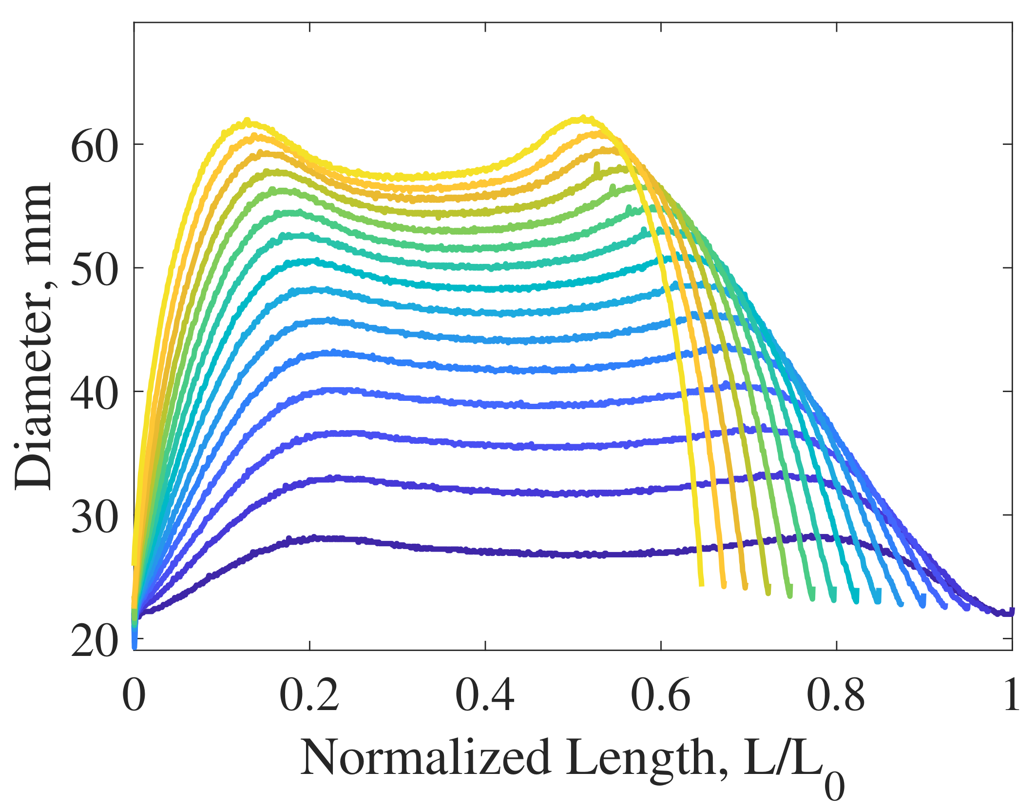
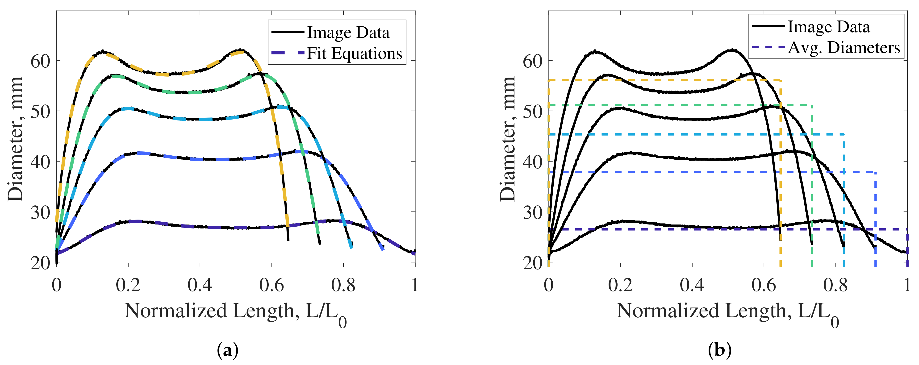
The average (mean) diameter is easily calculated from the raw shape profile data (Figure 13), and is the simplest representation of a shape profile for analysis. The mean diameter of the entire length of each traced outline is calculated. With the average defining a single diameter value for each profile, the resulting assumed cylindrical profile is in contrast to the complex curvature of the measured profile (Figure 14b). The average profiles result in average diameters that are about 10% below the maximum diameter due to the dramatic decrease in diameter at each end of the PAM in proximity to the end-fittings. The average diameter was calculated for the entire contraction range of the PAM at each pressure (Figure 15a). The results suggest that the radius is nominally independent of internal pressure. Closer inspection of the average diameters, however, reveals small increases in diameter with pressure. This is especially apparent in the zero-contraction state, where the diameter swells by about 0.5 mm from 20 psi to 100 psi. This appears to capture the affect of tensile stretching of the braid, a phenomenon that had not previously been captured. Stretching of the braid has often been ignored with a rigid braid assumption, but has also been accounted for—without the benefit of having quantitative data—in some modeling efforts [1,27]. Further investigation of the apparent increase of the braid diameter at fixed length states with increases in pressure warrants further investigation in future work.

5.1.2. Profile Fourier Series Fit

Previous assumed shape profiles have failed to accurately capture the complex curvature of the PAM’s shape profile. Piece-wise profile definitions used for attempted corrections on the cylindrical profile approximation—which typically use separate equations to define the profile of the midsection and the region near each end-fitting—increase modeling complexity with unvalidated improvements in accuracy. A single equation representation of the measured shape profiles is desired for simplicity of analysis.

Curve fit equations are used to fit the measured shape profiles. With multiple forms of fit functions to choose from (e.g., polynomial, exponential, etc.), it is important to select a function with a characteristic shape that resembles the shape of the observed profiles to enable an accurate and low-order fit equation. Since the observed profiles draw a resemblance to a half-sine pulse with higher-order harmonics, a Fourier series curve fit equation was selected. The form of the fit equation is given as:

$$y=a_0+\sum _{n=1}^3{a}_{n}cos\left(nxw\right)+b_{n}sin\left(nxw\right)$$

(7)

where x represents the position along the length of the shape profile, $a_0$ provides a horizontal shift, n indicates the order of the harmonic, and $a_n$ and $b_n$ are terms that scale the magnitude of each harmonic. Values of $a_0$, $a_n$, $b_n$, and w are found for each measured profile by performing a nonlinear least-squares fit (using MATLAB’s fit() function). The number of terms used for the fit is adjusted to achieve a good fit while also keeping the number of terms to a minimum for simplicity. A third-order Fourier series fit was found to achieve a very good fit of the shape profile data (Figure 14a). The resulting fit has a low combined average error for all tested states of contraction. The accuracy of the fit of this PAM begins to plateau with the use of three or more terms.

Table 2. The effect of the number of Fourier series fit terms used for fitting the profile data on the maximum and Root-Mean-Square Error (RMSE) averaged between all tested pressures.

Number of Terms	1	2	3	4	5
Avg. Max Error, mm	12.70	1.49	0.69	0.68	0.39
Avg. RMSE, mm	2.74	0.39	0.12	0.12	0.08

provides a comparison of the accuracy of the fit depending on the number of terms used. Values for each term of the three-term Fourier series fit performed in Figure 14a are provided in

Table 3. Coefficient values for the three-term Fourier Series fit performed in Figure 14a.

$\%{\mathit{L}}_0$	${\mathit{a}}_0$	${\mathit{a}}_1$	${\mathit{a}}_2$	${\mathit{a}}_3$	${\mathit{b}}_1$	${\mathit{b}}_2$	${\mathit{b}}_3$	w
0%	1.03	−0.08	−0.07	−0.02	0.02	0.04	0.02	5.72
8.75%	1.36	−0.36	−0.13	−0.00	−0.19	−0.21	−0.06	−5.78
17.5%	1.51	−0.57	−0.10	0.04	0.44	0.42	0.10	6.02
26.25%	1.16	−0.87	0.40	0.20	1.40	0.81	0.02	5.78
35%	−15.39	9.24	9.06	−1.82	25.68	−7.50	−1.08	3.81

. Some of the coefficient values found for the fit functions, as shown in Table 3, can appear to be erratic, and may require additional constraints on the fit function for smoother variations of parameters between measured profiles.

For a complete characterization, a fit function can be found for all of the profiles measured during tested states of pressures and contraction. As noted from previous observation of Figure 15a, the profile is predominantly a function of the contraction state with little variation with changes in pressure. This enables a reduction in the number of required fits to fully define the shape profile of the PAM by only needing to characterize the shape profiles of the maximum pressure tested.

5.1.3. Comparison to Previous Cylindrical Profile Estimates

The shape profile of PAMs has traditionally been modeled as a cylindrical profile. The diameter of the PAM can be estimated for all states of contraction by using this cylindrical approximation and an assumed initial geometry. The estimated profile diameter has long been assumed to be nominally accurate enough for use in almost all modeling efforts of PAMs. However, with no previous method of measuring the actual shape profile of PAMs, there has not been any quantifiable data to check the accuracy of these estimated cylindrical profiles until now. With the shape profile measurements acquired using photogrammetry, the accuracy of the cylindrical shape profile approximation can now be tested.

The cylindrical approximation has served as the basis of most PAM modeling since the inception of the PAM back in 1958 [28]. The cylindrical approximation, prior to the addition of any applied correction factors, makes the following assumptions:

• The shape profile is cylindrical (constant diameter with respect to length)
• The braid angle is constant with respect to length
• There is no strain in the braid fibers

With these qualifying assumptions, the geometry of the PAM can be defined using the triangle relationship which defines a set trigonometric relationship between the active length, L, diameter, D, and braid angle, $\theta$, of the PAM through fixed values that are the length of each braid fiber, B, and the number of turns of each braid fiber around the circumference of the PAM, N [4]. The fixed values of N and B, can then be found using the initial geometry of the PAM defined by the initial braid angle, ${\theta }_0$, the initial diameter, $D_0$, and the initial active length, $L_0$, through the following relations:

$$N=\frac{L_0}{D_0\pi tan\left({\theta }_0\right)}$$

(8)

$$B=\frac{L_0}{sin\left({\theta }_0\right)}$$

(9)

Finally, the diameter of the PAM can be estimated as a function of active length through the following relationship:

$$D_{est}\left(L\right)=\frac{\sqrt{B^2-L^2}}{\pi N}$$

(10)

The established direct relationship between $D_{est}$ and L produces estimated diameter values—commonly used as an input parameter to models—through relatively simple geometric relationships. However, it is also relatively sensitive to the assumed initial geometry of the PAM. The value of $D_0$ is commonly assumed to be equal to the resting outer diameter of the bladder (assuming a thin braid), or the braid diameter at its point of insertion into the end-fitting. The value of ${\theta }_0$ can then be determined using the method covered in Pillsbury, (2015) [29] which uses the linear relationship between blocked force and pressure to solve for ${\theta }_0$. It should be noted that the value of ${\theta }_0$ found through this method is a function of the estimated value of $D_0$.

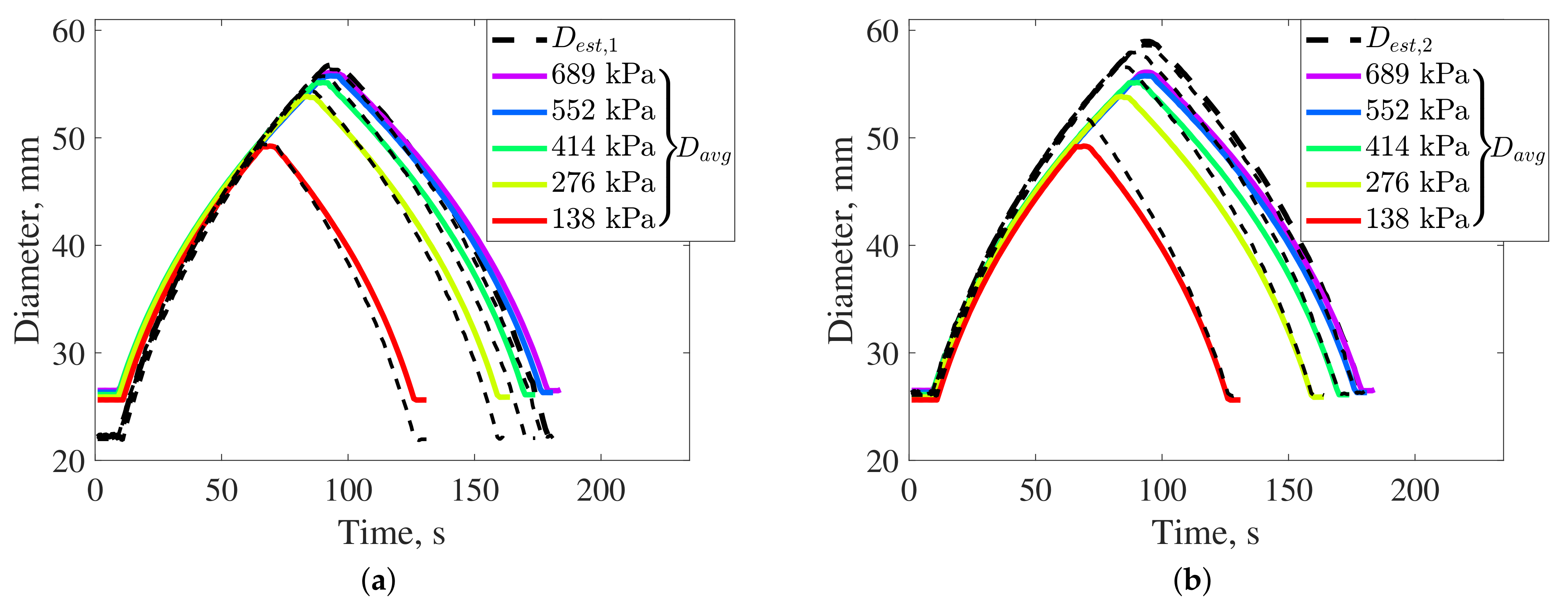
The average diameter of the measured profile data will be compared to the estimated cylindrical profile. The assumed cylindrical profiles for both the estimated and average of the measured data provide a basis of direct comparison. An accurate estimated profile diameter should match the average of the measured profiles.

The value of $D_0$ for the tested PAM is equal to the outer diameter of the bladder at 22.2 mm (7/8 in). An estimated value of ${\theta }_0$ was found using the blocked force with respect to pressure data to be 72.27 degrees. The resulting estimated diameter values, labeled as $D_{est,1}$, are compared to the results of the measured data in Figure 16a for a single stroke of the PAM. There is an observed error in the estimated value of $D_0$ which is about 3.8 mm (0.15 in) below the initial measured average diameter of about 26.0 mm (1.025 in). This initial increase in diameter was not due to any noticeable slack in the braid prior to pressurization, with the braid being taut in the resting length state. The resulting discrepancy between the estimated and measured diameters is especially large at low levels of contraction.

With knowledge of the actual value of $D_0$, using the measured data we can attempt to estimate the shape profile again with corrected values of $D_0$ and ${\theta }_0$. Since there is a slight range of the measured initial diameter values with respect to pressure, the average of these measured values of 26.0 mm (1.025 in) can be used for this comparison. This value of $D_0$ results in a value of 69.04 degrees, a significant difference from the previous value of 72.27 degrees. Estimated diameter values, $D_{est,2}$, are calculated using the new initial geometry conditions (Figure 16b). With proper alignment of the curves at low levels of contraction, there is now a sizeable error in the maximum contraction state. The resulting error between curves could be the result of the estimated value of ${\theta }_0$ being too high. A lower value of ${\theta }_0$ would result in lower values of estimated maximum contraction. If the value of ${\theta }_0$ is reduced to 68–68.5 degrees with $D_0$ still equal to 26.0 mm, the estimated and measured diameter curves match very well. However, an accurate physical measurement of the value of N for the tested PAM found that the braid angle should be around 68.9–69.7 degrees which coincides well with the value of ${\theta }_0$ used to define $D_{est,2}$. It is therefore likely that the discrepancy between the values of $D_{avg}$ and $D_{est,2}$ are a result of error from using the cylindrical approximation for the estimated diameter values. The cylindrical approximation, in estimating a diameter from the initial geometry state, neglects the length of the braid that is effectively lost to the curvature of the PAM’s braid resulting in overestimates of the estimated diameter. This research serves as an initial comparison of these estimated and measured diameter values, with the resulting discrepancy between these values deserving of further investigation.

5.2. Volume Approximation

Measurement of a PAM’s internal volume is often required for actuation system design and modeling efforts. Estimates of volume are necessary to determine requirements of the system such as the working fluid flow rate and storage requirements. Modeling efforts also use values of internal volume for force-response models (e.g., virtual work method), as well as for providing estimates of actuation efficiency. The acquisition of accurate volume measurements has often proved difficult for researchers due to the specialized equipment that is often required to do so. As a consequence, researchers have often settled for using dimensions provided by using the estimated cylindrical approximation diameter.

The photogrammetric data acquired in this research provides the opportunity to easily obtain an accurate estimation of the internal volume of the PAM for all tested pressure and contraction states. Since the profiles only provide a two-dimensional depiction of the PAM, a three-dimensional measurement of volume requires the assumption that the PAM is axisymmetric about its longitudinal axis. The symmetry of many previously tested PAMs usually makes this a reasonable assumption. Appreciable deviations from symmetry have only been observed for PAMs with flaws in their fabrication.

Using the shape profile data, the internal volume of the PAM, $V_{int}$, can be found using the following basic equation:

$$V_{int}=V_{prof}-V_{bld}-V_{brd}$$

(11)

where,

$$V_{prof}=\left\{\begin{array}{cc}{w}_p\sum _{i=1}^{L_p}\frac{\pi }{4}{D}_i^2,\hfill & \mathrm{discrete}\mathrm{profile}\hfill \\ \\ \pi {\int }_0^L{\left(\frac{D\left(x\right)}{2}\right)}^{2}dx,\hfill & \mathrm{continuous}\mathrm{profile}\hfill \end{array}\right.$$

(12)

$V_{prof}$ is the volume encased within the outline of the shape profile of the PAM, $V_{bld}$ is the volume consumed by the incompressible bladder, and $V_{brd}$ is the volume of the braid. Therefore, Equation (11) states that the internal volume of the PAM is equal to the volume within the shape profile minus the volumes of the bladder and braid that are also contained within the shape profile volume. The bladder and braid volumes are fixed values that can easily be found using their cylindrical dimensions in the PAM’s resting length configuration (i.e., $L_0$). For the PAM used in this research, the braid has an assumed resting diameter of 21.9 mm (0.863 in) equal to that of the end-fitting at each end, and a thickness of 0.28 mm (0.011 in) resulting in a value for $V_{brd}$ of 4.47 cm${}^3$ (0.273 in${}^3$). The incompressible bladder has a resting outer diameter of 22.2 mm (7/8 in) and thickness of 1.6 mm (1/16 in), resulting in a bladder volume, $V_{bld}$, of 24.26 cm${}^3$ (1.481 in${}^3$).

The volume $V_{prof}$ can be found through integration of the defined shape profile (Equation (12)). The method of integration is dependent on how the shape profile is defined. In this paper, the diameter of the shape profile has been defined as a discrete function $D_i$, with the width of the PAM defined for each pixel i along the length of the PAM, and as a continuous function, $D\left(x\right)$, defined by the Fourier series fit equations used to describe the shape profile of the PAM. To find $V_{prof}$ for the discrete definition of the shape profile, integration is performed as a summation of the volume of each pixel-width slice of the PAM. This discrete integration is shown in Equation (12), where $w_p$ is the width of each pixel, and $L_p$ is the current length (in pixels) of the PAM. The continuous function definition of the shape profile provides a much simpler method of calculating the volume of the PAM. As shown in Equation (12), disc integration is performed to calculate the volume $V_{prof}$ using the continuous function form of the shape profile, $D\left(x\right)$. The cylindrical approximated diameter of the PAM, $D_{cyl,fit}$, having been shown to accurately represent the average diameter of the PAM, can also be used to calculate the volume $V_{prof}$ of the PAM.

Using the discrete form of the shape profile data, the internal volume of the tested PAM is calculated as shown in Figure 15b. As is predicted from the average shape profile diameter results of Figure 15a, the volume is a function of the length state of the PAM and is effectively independent of internal pressure. There is only a slight deviation in volume with respect to pressure due to the assumed stretch in the braid. These results can be easily adjusted to provide values for the change in volume required for contraction of the PAM as would be needed for flow rate and efficiency calculations.

5.3. Testing of Different PAMs

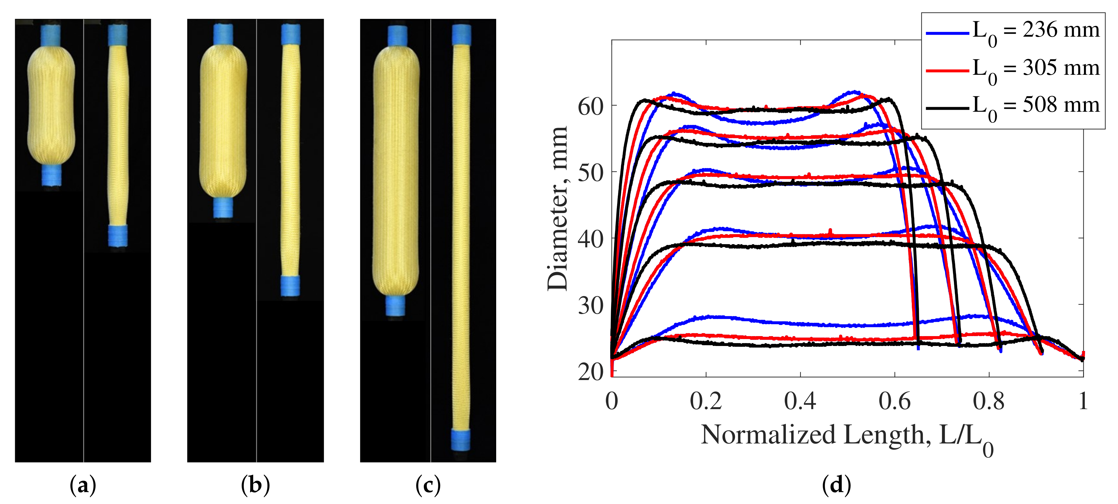
A few other PAMs have been characterized thus far using the photogrammetric methods as described above. Three 22.2 mm (7/8 in) diameter PAMs and one 57.2 mm (2 1/4 in) diameter PAM have been characterized using photogrammetry. The three 22.2 mm diameter PAMs have identical material construction. 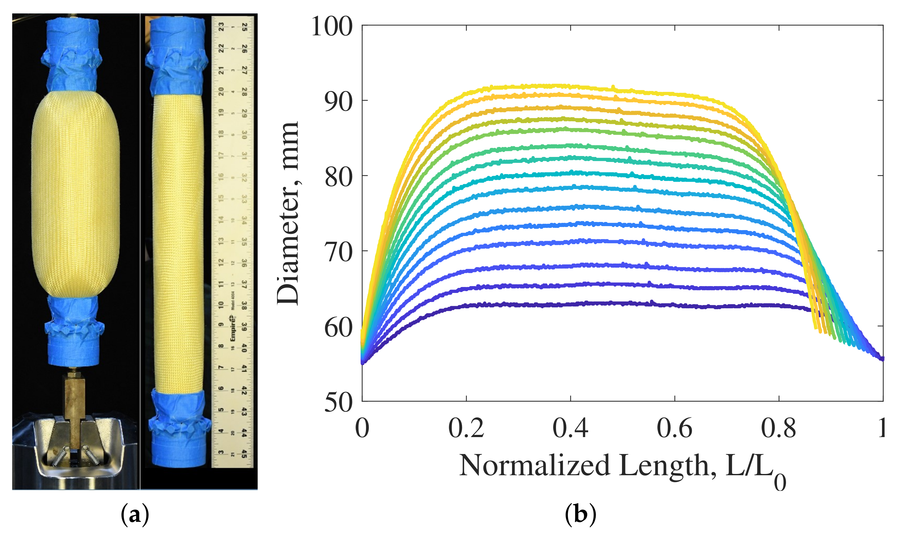The 236 mm (9 9/32 in) long PAM has been used to demonstrate the photogrammetric methods up to this point, and PAMs with 305 mm (12.0 in) and 508 mm (20.0 in) lengths have also been tested (Figure 17). These PAMs were tested to compare their shape profiles while also demonstrating the ability of the photogrammetric test setup to characterize PAMs of varying length scales. Analysis of the 57.2 mm diameter by 351 mm (13 13/16 in) long PAM (Figure 18) further demonstrates the capability of the test method to characterize PAMs of a wide range of diameters.

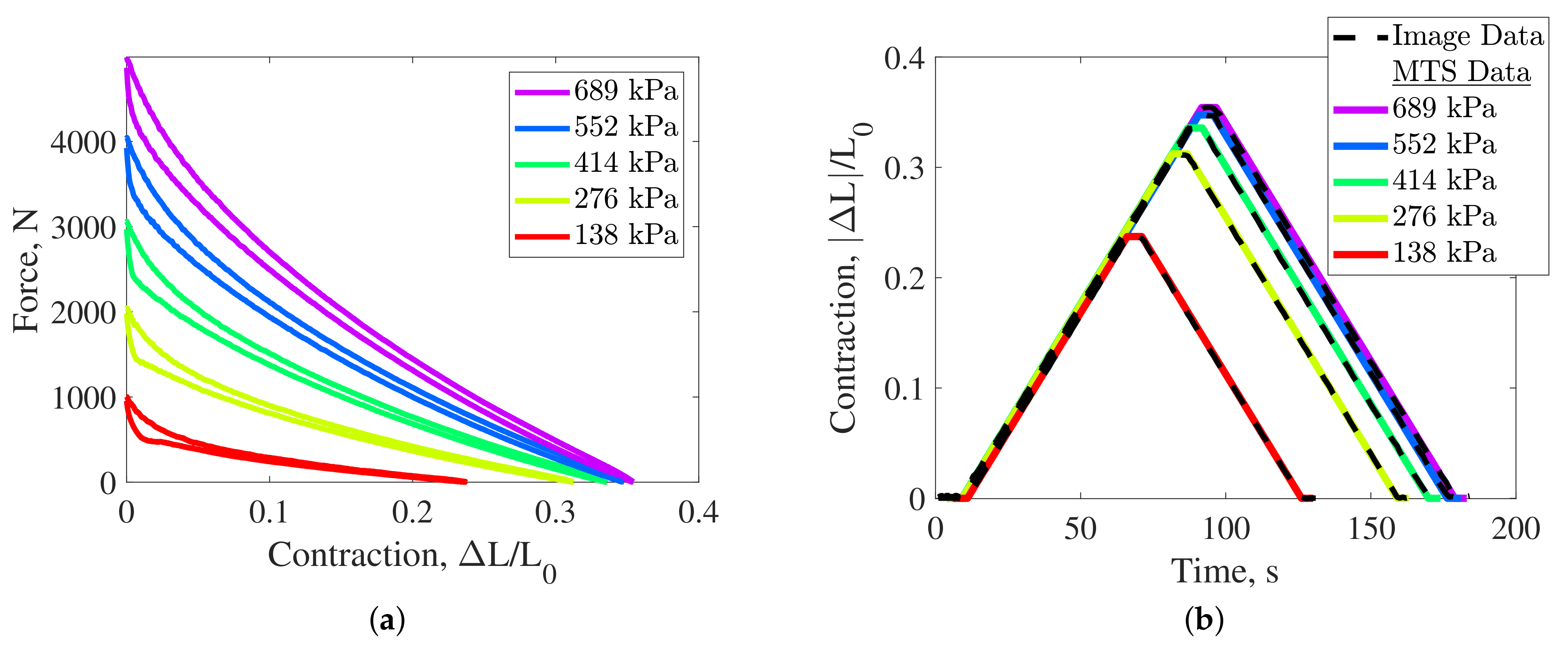
The shape profiles of the 22.2 mm diameter PAMs are compared in Figure 17d for the same five states of percent contraction. Despite their slight differences in shape, their resulting diameters are very similar. The three PAMs were all able to achieve nearly identical free contraction values at 689 kPa (100 psi) of 35.43%, 35.55%, and 35.36% for the 236 mm, 305 mm, and 508 mm PAMs, respectively. Each of their profiles has an undulation at each end of the PAM that resembles the previously noted peanut-like shape which seems to be a characteristic of many PAMs. The shape profile of the 508 mm (longest) PAM has an additional small undulation at its mid-length that is barely visible. A Fourier series fit was conducted on the three PAMs resulting in an accurate representation of their profiles. A three-term Fourier series provides an accurate fit for the 236 mm and 305 mm long PAMs, while the additional undulation of the 508 mm long PAM profile requires a four-term Fourier series to achieve a good fit. The largest discrepancy between the profiles comes in the zero-percent contraction state, where the 236 mm PAM has the largest average diameter of the three. The difference in initial diameters is reflected by the difference in their estimated initial braid angles. The three PAMs had estimated initial braid angles of 69.4, 71.1, and 71.9 degrees for the 236 mm, 305 mm, and 508 mm PAMs, respectively. With all three PAMs using the same braid, the differences in initial braid angle and diameter indicates slight differences in their fabrication or identification of their resting length. As previously noted from observation of Figure 15a, the diameter of the PAM is much more sensitive to changes in length at lower states of contraction, so a small deviation in length or braid angle near the resting length state results in a relatively large change in the expected diameter.

The shape profiles of the 57.2 mm diameter PAM, as shown in Figure 18b, are also accurately captured using the described photogrammetric methods. The simpler rounded shape of its profile allows for an accurate Fourier series fit of the profiles to be achieved with the use of only two terms.

Testing of both the 22.2 mm diameter by 508 mm long PAM, and the 57.2 mm diameter by 351 mm long PAM, represents the maximum extent of what has been produced with regard to sizing of PAM lengths and diameters, respectively. Although the photogrammetric measurement of PAMs of different sizes might seem trivial, many previous test setups for PAM volume testing have required modifications or redesigns in order to administer tests for PAMs of different sizes. Photogrammetric characterization is capable of testing PAMs with a large range of sizes by just repositioning the camera to capture and fill each image with the entire PAM. As mentioned earlier, the positioning of the camera will effect the accuracy of the photogrammetric measurements. The accuracy is dependent on the competing effects of attempting to reduce the angle-of-view by distancing the camera from the PAM, while also keeping the distance at a minimum to maximize measurement resolution. For the 22.2 mm diameter PAMs, the camera was setup at the distance of 152 cm (60 in) for the shorter 236 mm length PAM, and it was placed 7.6 cm (3.0 in) farther away for the longer 508 mm PAM to capture its entire length. Those two camera placements resulted in angle-of-views of 8.84 and 18.04 degrees, respectively, and measurement resolutions of 8.52 pixels/mm (216.35 pixels/in) and 8.92 pixels/mm (226.63 pixels/in), respectively. Both tests achieved a high degree of accuracy despite the slight changes in resolution and angle-of-view. Comparing the contraction measurements of the MTS machine and photogrammetric data, as performed in Figure 12b for the 236 mm PAM, resulted in a maximum error of 0.61 mm (0.042 in) (0.21%) for the 508 mm long PAM. This is in comparison to the 0.60 mm (0.024 in) (0.25%) error previously cited for the 236 mm PAM. Similarly, measurement of the 57.2 mm diameter PAM achieved results with a maximum error in the length contraction measurement of 1.3 mm (0.05 in) (0.36%). It is assumed that even with the larger diameter of this 57.2 mm PAM, its diameter is still significantly smaller than the length measurement that is used here to cap the maximum expected error in the measurement.

The accurate characterization of the shape profiles of the four PAMs demonstrates that the photogrammetric methods presented in this research can be readily adapted to PAMs of different length and diameter scales. A new method of experimentally characterizing the volume of PAMs has been presented that can be performed without the need for specialized test equipment, and can be easily adapted for the measurement of PAMs of different sizes.

6. Conclusions

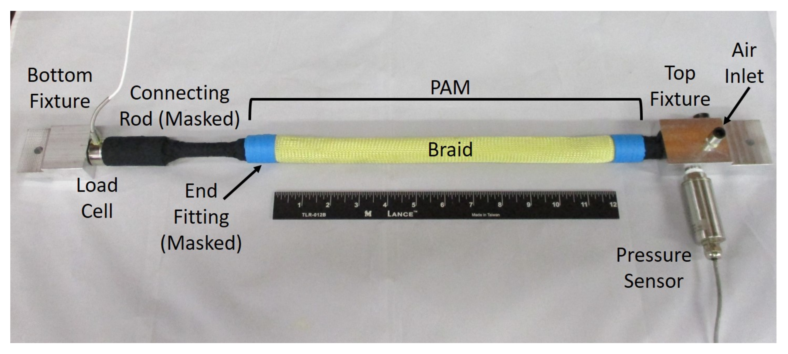
This research presents an approach for characterizing the shape profile of PAMs through photogrammetric measurement. The method of measuring the PAM’s shape profile is described including a basic test setup, method of image acquisition, and a process of abstracting measurements from the image data. A 22.2 mm diameter PAM served as an example for describing the presented test method and analysis.

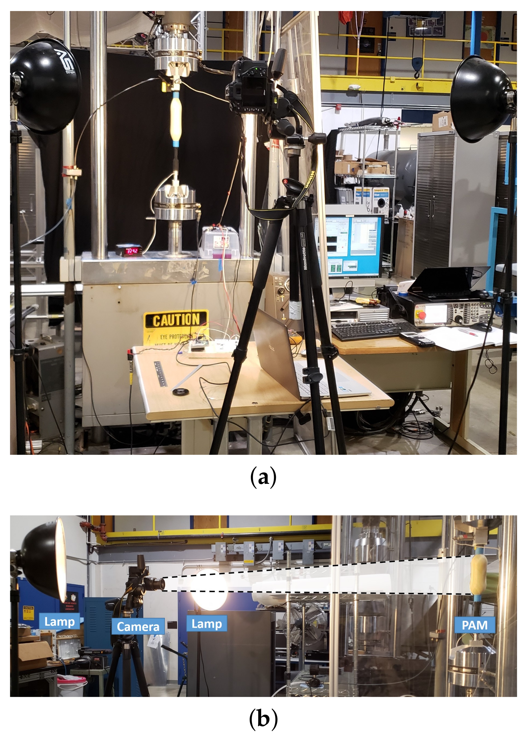
The photogrammetric testing was performed in parallel with the isobaric force-contraction characterization that is typically performed to define the actuation of PAMs. The photogrammetric test setup requires the addition of only a camera, backdrop, lighting, and masking to acquire measurement data. The complete method of acquiring measurements from the image data, including a background on the methods used, was provided in detail to ease the adoption of this characterization method for future research efforts.

Some preliminary analysis of the shape profile data was then performed. The average diameter and volume of the PAM were found to be primarily a function of the contraction state. However, there was an indication of strain in the braid fibers from the small but appreciable increase in PAM diameter with increased pressure. This strain in the braid fibers had not been quantifiable prior to the characterization performed in this testing. The measured shape profiles were redefined from a set of data points to a cylindrical approximation or fit equation. The average of each measured profile was used to define each profile as a single value. This assumes a cylindrical shape profile that can be readily applied to previously existing models. If the assumption of a cylindrical shape profile is not sufficient for a high-fidelity modeling effort, the complex curvature of the shape profiles can be defined to a high-degree of accuracy using Fourier series fit equations. Working with equations instead of the raw shape profile data greatly simplifies usage of the shape profile information garnered from the photogrammetric testing.

The estimated diameters found using the cylindrical approximation and initial geometry have long served as the basis for most PAM modeling. These estimates were tested by comparing them to the measured average diameters of the tested PAM. The comparisons resulted in discrepancies between the estimated and measured diameters, with the first comparison finding an inaccuracy in the initial estimated diameter. After this initial offset in diameter was corrected, the estimated diameters still did not match the measured diameters, warranting further future investigation of the effect of the cylindrical approximation on these estimates.

A new method of characterizing the internal volume of PAMs using the acquired shape profile data was also presented. This new non-contact method of calculating the internal volume is desirable compared to current methods which often require specialized test equipment that must be altered in order to test PAMs of different sizes.

Finally, the accuracy and adaptability of the presented test method is demonstrated through the shape profile characterization of multiple PAMs of different sizes. A comparison of three 22.2 mm diameter PAMs was performed, demonstrating some of the similarities in their contraction-diameter characteristics, and also the slight differences in the undulations and curvature of their profiles. A wide 57.2 mm PAM was also accurately characterized with the same test setup without the need for any modifications. The Fourier series fit was able to accurately replicate the profile data for all tested PAMs with an observed correlation between the number of undulations of the profile’s curvature, and the number of terms required to provide an accurate fit.

The presented method was developed out of a need to be able to quantify modeling unknowns and long-used estimations of diameter, but also out of the necessity to define the dimensions of PAMs for implementation into mechanism designs, and define system requirements for the PAM’s supporting hardware. The shape profile data this new method provides can also be used to improve the accuracy of actuation force model inputs—such as diameter, braid angle, bladder strain, and braid strain—which currently rely on cylindrical approximations of the PAM’s shape profile, and empirically-based modeling corrections. It is the authors hope that this method of characterization can aid in the discovery, confirmation, and necessary adjustments for improved modeling efforts, as well as enlighten and ease the adoption of PAMs by providing a more complete characterization of their actuation.

References

1. Kothera, C.S.; Jangid, M.; Sirohi, J.; Wereley, N.M. Experimental characterization and static modeling of McKibben actuators. J. Mech. Des. 2009, 131, 091010. [Google Scholar] [CrossRef]
2. Robinson, R.M.; Kothera, C.S.; Wereley, N.M. Quasi-static nonlinear response of pneumatic artificial muscles for both agonistic and antagonistic actuation modes. J. Intell. Mater. Syst. Struct. 2015, 26, 796–809. [Google Scholar] [CrossRef]
3. Carlo Ferraresi, W.F.; Walter Franco, W.; Bertetto, A. Flexible pneumatic actuators: A comparison between the McKibben and the straight fibres muscles. Rob. Mechatron. 2001, 13, 56–63. [Google Scholar] [CrossRef]
4. Chou, C.P.; Hannaford, B. Measurement and modeling of McKibben pneumatic artificial muscles. IEEE Trans. Robot. Autom. 1996, 12, 90–102. [Google Scholar] [CrossRef] [Green Version]
5. Hocking, E.G.; Wereley, N.M. Analysis of nonlinear elastic behavior in miniature pneumatic artificial muscles. Smart Mater. Struct. 2012, 22, 014016. [Google Scholar] [CrossRef]
6. Tiwari, R.; Meller, M.A.; Wajcs, K.B.; Moses, C.; Reveles, I.; Garcia, E. Hydraulic artificial muscles. J. Intell. Mater. Syst. Struct. 2012, 23, 301–312. [Google Scholar] [CrossRef]
7. Tondu, B.; Lopez, P. Modeling and control of McKibben artificial muscle robot actuators. IEEE Control Syst. Mag. 2000, 20, 15–38. [Google Scholar]
8. Tsagarakis, N.; Caldwell, D.G. Improved modelling and assessment of pneumatic muscle actuators. In Proceedings of the 2000 ICRA. Millennium Conference. IEEE International Conference on Robotics and Automation. Symposia Proceedings (Cat. No. 00CH37065), San Francisco, CA, USA, 24–28 April 2000; Volume 4, pp. 3641–3646. [Google Scholar]
9. Meller, M.A.; Bryant, M.; Garcia, E. Reconsidering the McKibben muscle: Energetics, operating fluid, and bladder material. J. Intell. Mater. Syst. Struct. 2014, 25, 2276–2293. [Google Scholar] [CrossRef]
10. Woods, B.K.; Kothera, C.S.; Wereley, N.M. Wind tunnel testing of a helicopter rotor trailing edge flap actuated via pneumatic artificial muscles. J. Intell. Mater. Syst. Struct. 2011, 22, 1513–1528. [Google Scholar] [CrossRef]
11. Linder, W. Digital Photogrammetry; Springer: Berlin, Germany, 2009. [Google Scholar]
12. Luhmann, T.; Robson, S.; Kyle, S.; Harley, I. Close-Range Photogrammetry and 3D Imaging. Available online: https://www.degruyter.com/document/doi/10.1515/9783110607253/html (accessed on 2 March 2021).
13. Cardani, D. Adventures in Hsv Space; Laboratorio de Robótica, Instituto Tecnológico Autónomo de México. 2001. Available online: http://citeseerx.ist.psu.edu/viewdoc/download?doi=10.1.1.456.1142&rep=rep1&type=pdf (accessed on 2 March 2021).
14. Skarbek, W.; Koschan, A.; Bericht, T.; Veroffentlichung, Z.; Klette, P.D. Colour Image Segmentation—A Survey. 1994. Available online: http://citeseerx.ist.psu.edu/viewdoc/summary?doi=10.1.1.28.1325 (accessed on 2 March 2021).
15. Schwarz, M.W.; Cowan, W.B.; Beatty, J.C. An experimental comparison of RGB, YIQ, LAB, HSV, and opponent color models. ACM Trans. Graph. 1987, 6, 123–158. [Google Scholar] [CrossRef]
16. Smith, A.R. Color gamut transform pairs. ACM SIGGRAPH Comput. Graph. 1978, 12, 12–19. [Google Scholar] [CrossRef]
17. Srinivasan, G.; Shobha, G. Segmentation techniques for target recognition. Int. J. Comput. Commun. 2007, 1, 313–333. [Google Scholar]
18. Nishad, P. Various colour spaces and colour space conversion. J. Glob. Res. Comput. Sci. 2013, 4, 44–48. [Google Scholar]
19. Canny, J. A computational approach to edge detection. IEEE Trans. Pattern Anal. Mach. Intell. 1986, 679–698. [Google Scholar] [CrossRef]
20. Liu, D.; Yu, J. Otsu method and K-means. In Proceedings of the 2009 Ninth International Conference on Hybrid Intelligent Systems, Shenyang, China, 12–14 August 2009; Volume 1, pp. 344–349. [Google Scholar]
21. Otsu, N. A threshold selection method from gray-level histograms. IEEE Trans. Syst. Man Cybern. 1979, 9, 62–66. [Google Scholar] [CrossRef] [Green Version]
22. Reddy, P.R.; Amarnadh, V.; Bhaskar, M. Evaluation of stopping criterion in contour tracing algorithms. Int. J. Comput. Sci. Inf. Technol. 2012, 3, 3888–3894. [Google Scholar]
23. Pradhan, R.; Kumar, S.; Agarwal, R.; Pradhan, M.P.; Ghose, M. Contour line tracing algorithm for digital topographic maps. Int. J. Image Process. 2010, 4, 156–163. [Google Scholar]
24. Pillsbury, T.E.; Wereley, N.M.; Guan, Q. Comparison of contractile and extensile pneumatic artificial muscles. Smart Mater. Struct. 2017, 26, 095034. [Google Scholar] [CrossRef]
25. Chambers, J.M.; Carignan, C.R.; Wereley, N.M. Powering a Lower Limb Exoskeleton Using Pneumatic Artificial Muscles. In Proceedings of the ASME 2016 International Mechanical Engineering Congress and Exposition, Phoenix, AZ, USA, 11–17 November 2016. [Google Scholar]
26. Chambers, J.M.; Wereley, N.M. Influence of hydraulic versus pneumatic working fluids on quasi-static force response of fluidic artificial muscles. J. Intell. Mater. Syst. Struct. 2021, 32, 385–396. [Google Scholar] [CrossRef]
27. Davis, S.; Tsagarakis, N.; Canderle, J.; Caldwell, D.G. Enhanced modelling and performance in braided pneumatic muscle actuators. Int. J. Robot. Res. 2003, 22, 213–227. [Google Scholar] [CrossRef]
28. Gaylord, R.H. Fluid Actuated Motor System and Stroking Device. U.S. Patent 2,844,126, 22 July 1958. [Google Scholar]
29. Pillsbury, T.E.; Kothera, C.S.; Wereley, N.M. Effect of bladder wall thickness on miniature pneumatic artificial muscle performance. Bioinspir. Biomim. 2015, 10, 055006. [Google Scholar] [CrossRef] [PubMed] [Green Version]
Figure 1. PAM with its braid traced along its edge (green), defining the shape profile of the PAM.
Actuators 10 00072 g001
Figure 2. Variation of the PAM’s shape profile for: (a) A single PAM in different states of contraction. (b) Three different PAMs (same construction) in their free-contraction states.
Actuators 10 00072 g002
Figure 3. Comparison of PAM shape profiles: (a) Actual shape profile, with varying radius along its length. (b) The cylindrical approximation profile that is commonly assumed, with constant radius along its length.
Actuators 10 00072 g003
Figure 4. Cylindrical HSV color space.
Actuators 10 00072 g004
Figure 5. Example depiction of Moore-Neighbor boundary tracing. (a) Moore-Neighborhood of pixel C, and prior boundary pixel P. (b) Tracing of a pixel cluster by stepping through pixels 1–8.
Actuators 10 00072 g005
Figure 6. PAM with sensors, MTS fixtures, and masking applied prior to mounting in the MTS machine.
Actuators 10 00072 g006
Figure 7. (a) Front, and (b) Side views of the photogrammetric test setup (PAM, camera, lights, and backdrop).
Actuators 10 00072 g007
Figure 8. Method of image scale calibration using ruler: (a) Original image view (5569 × 3712 pixels). (b) Cropped image view (2650 × 1100 pixels). (c) Identification of ruler 1/8 in increment hatch marks. (Top) Each hatch mark has its left (blue), right (green), and then center (red) located. (Bottom) Locating respective points of each hatch mark is performed through analysis of the brightness (V) gradient.
Actuators 10 00072 g008
Figure 9. Identification of the PAM in the image: (a) Initial image. (b) Step 1a: Pixel segmentation histogram using Otsu’s method to set threshold on brightness (V). (c) Step 1b: V segmented binary image. (d) Step 2: Traced outline of PAM.
Actuators 10 00072 g009
Figure 10. Identification of the end-fittings in the image: (a) Image of PAM only. (b) Step 3a: Pixel segmentation histogram using Otsu’s method to set threshold on Hue (H). (c) Step 3b: H segmented binary image. (d) Step 4: End-fittings outline traced.
Actuators 10 00072 g010
Figure 11. The resulting shape profile of the braid along the PAM’s length. (a) Step 5: Profile; (b) Diameter of shape profile with respect to length.
Actuators 10 00072 g011
Figure 12. Test results of the 236 mm long, 22.2 mm diameter test PAM: (a) Actuation diagram. (b) Comparison between contraction values found from the image data using photogrammetry, and the displacement values recorded by the MTS machine. Results are shown for a single contraction cycle at all tested pressures.
Actuators 10 00072 g012
Figure 13. Evolution of the PAM’s shape profile for its full contraction range at 689 kPa (100 psi).
Actuators 10 00072 g013
Figure 14. Comparison of assumed profiles to the measured shape profiles of the PAM at 0, 8.75, 17.5, 26.25, and 35 (maximum) percent contraction at 689 kPa (100 psi): (a) Three-term Fourier series fit equation profiles. (b) Assumed cylindrical profiles that have diameters equal to the average diameter of the respective measured shape profiles.
Actuators 10 00072 g014
Figure 15. Initial analysis of the measured profiles for the full contraction ranges of 139–689 kPa (20–100 psi) tests: (a) Average diameter. (b) Internal air volume.
Actuators 10 00072 g015
Figure 16. Comparison of the average measured diameter values, D a v g , against estimated diameters, D e s t : (a) D e s t , 1 (Initial geometry: D 0 = 22.2 mm, θ 0 = 72.27 deg.). (b) D e s t , 2 (Initial geometry: D 0 = 26.0 mm, θ 0 = 69.04 deg.)
Actuators 10 00072 g016
Figure 17. Shape profile comparison for PAMs of different lengths: (a) L 0 = 236 mm. (b) L 0 = 305 mm. (c) L 0 = 508 mm. (d) Comparison of their shape profiles at 0, 8.75, 17.5, 26.25, and 35 percent contraction (689 kPa (100 psi)). The profiles have approximately equivalent diameters with slight differences in shape.
Actuators 10 00072 g017
Figure 18. Characterization of the 57.2 mm diameter PAM at 179 kPa (26 psi): (a) Free contraction and resting length states. (b) Evolution of the PAMs shape profile.
Actuators 10 00072 g018