1. Introduction
Fluidic artificial muscles (also known as pneumatic artificial muscles when they are operated with air) are soft actuators shown to have high specific power and long fatigue lifetimes [
1,
2,
3]. With much greater elasticity and tolerance to large deformations than linear or rotational electric actuators, fluidic artificial muscles (FAMs) can be categorized as a subgroup of soft actuators. They are characterized by their simple design, no parts moving through seals or bearings, and inherent compliance, which relaxes the requirements on precise alignment.
FAMs were first patented by R.H. Gaylord (1958) [
4] and later popularized by J.L. McKibben in the 1960s. Initially, due to advances in electric motor miniaturization, FAMs (also called McKibben muscles) started to lose their popularity in robotics and prosthetics research. It was not until the late 1980s, when a Japanese tire manufacturer, Bridgestone, patented its more powerful McKibben muscles and introduced the soft robotic manipulators “soft-arms” for painting applications [
5,
6,
7] that the FAMs regained popularity and a broad research interest was revived. The range of applications has been expanding ever since. However, due to their subtle physics and outstanding performance, FAMs remain an area of active research.
A FAM is composed of four components: an elastomeric tube, a braided sleeve, and two end fittings, as shown in
Figure 1a. The elastomeric tube is fitted into the braided sleeve, and then joined together at both ends with pressure-tight sealed end fittings. One of the end fittings has a channel for the fluid input and is typically fixed, while the other serves as the force attachment point. When inflated, the muscle changes its length, and contracts or extends depending on its resting braid angle. This braid angle describes the angle between its radius and the fiber direction, as shown in
Figure 1a. A FAM is contractile if the braid angle is larger than
°, or extensile if the braid angle is smaller than
° [
8]. The commonly modeled behavior of contractile and extensile FAMs is shown in
Figure 2a,b.
Contractile FAMs (CFAMs) are able to generate blocked forces that are ten times greater than the force output of a pneumatic cylinder of comparable diameter and operating pressure. As the braid angle approaches 0, Equation (
1) becomes a simplified force equation for a pneumatic cylinder. In
Figure 3, it can be shown that the CFAM reaches a normalized blocked force of 10 for a braid angle lower than 70° as compared to the value of 1 for a braid angle of 0. The blocked force is here defined as the force generated by a FAM when its length is fixed to its resting length. A resting length is the length of a FAM when there are no external forces acting on the actuator and its internal pressure is zero. Unlike contractile FAMs, which were reported to reach normalized length changes between 24% and 35% for pressures of up to 690 kPa [
9,
10], extensile FAMs (EFAMs) can provide much larger strokes that exceed their initial length. Theoretically, 200% extension can be achieved at a braid angle of 22° [
11], although in practice stroke values of up to 80% have been reported [
9,
12].
1.1. FAM Static Behavior
To understand FAMs (or McKibben muscles), let us first imagine an infinitely long muscle in which the fibers are not angled, but rather go straight from one end fitting to another. When a straight-fiber muscle is pressurized, the interior pressure acts radially on its elastic bladder walls. The walls, surrounded by the braided sleeve, transfer this force onto the fibers, which convert the radial force to an axial force. This axial force pulls in on the muscle’s end fittings, forcing the system to find a new equilibrium with shorter length and larger diameter. As the axial force contracts the muscle, the bladder strains both axially and radially. Though this straight-fiber muscle generates much greater force than the McKibben muscle, as highlighted by Ferraresi et al. (2001) [
13], the resulting material strain exceeds allowable values for rubber.
The excess strain is not an issue with McKibben muscles, where the radial force is not fully converted to the axial direction. The axial force drops as the muscle shortens and the braid angle decreases (see Equation (
1)). In extensile FAMs, a smaller braid angle corresponds to a greater magnitude axial force, as opposed to contractile FAMs in which larger braid angles correspond to larger magnitude axial forces (see
Figure 3). In EFAMs, when the pressure acting on the walls transfers the force onto the fibers, only a small part of that force is converted into the pulling force as the braid now mostly counteracts radial expansion. Since the pressure acting on the inner surface of the end fittings produces a greater pushing force than pulling force in the fibers, the EFAM is forced to a new equilibrium with a greater length, larger braid angle, and smaller outer diameter. According to, Gaylord’s blocked force equation:
where
stands for the blocked force,
P stands for the FAM internal pressure,
stands for the resting braid angle, and
D denotes the resting outer diameter. The equation was further described in
Section 4.
Note that for a braid angle of °, the blocked force changes its sign. This boundary separates the extensile FAM from the contractile FAM. To put things into perspective, a pneumatic cylinder of some diameter, D, would generate a normalized force equal to 1. A contractile FAM of the same diameter, D, would generate larger blocked forces than the force output of the cylinder for braid angles greater than . An extensile FAM’s blocked force reaches the force output of the pneumatic cylinder as the braid angle approaches 0.
1.2. Literature on FAM Modeling
FAMs offer the power and reliability of electric actuators that no other chemo- mechanical artificial muscles can provide [
14,
15], and have been widely used in robotic and aerospace applications [
1,
2,
3,
11,
16,
17,
18]. However, the applications of EFAMs, specifically, have been rather limited. Primarily, their application has been found in continnum soft robots and secondarily in power assistive devices and soft grippers. In continuum soft robots, EFAMs can be parallelly bundled to create a flexible beam-like structure that bends and extends when a differential pressure is applied to the muscles [
19,
20,
21,
22,
23,
24]. Another approach to achieve out-of-axis motion is to constrain an EFAM from extending on one side or helically. This way FAMs with bending and helical motions were produced, and later applied to a gripper [
25] and a continuum robot [
26]. Another application was also found in an assistive exoskeleton glove where bending EFAMs were attached to the top of the glove along human test subject’s major hand joint (metacarpophalangeal) and its fingers. It was shown that the glove reduced subject’s effort in a grasping task [
27,
28,
29].
For its various applications, several analyses have been proposed to model the actuator, with two prominent models being the energy balance model [
6,
30,
31,
32] and the force balance model [
13,
33]. These models were later extended with a non-cylindrical shape at the ends of the actuator [
34], friction force [
30], strain-stiffening effect [
34], pressure-dependent stress functions [
9], and actuated pressure correction (or dead-band pressure) [
16,
30,
34]. There is a fundamental difference between the basic energy balance model, and the force balance model employed in this study. The standard energy balance model is defined using the equation [
6]:
where
is the strain,
F is the force generated by a FAM,
P is the internal pressure,
is the resting outer radius,
is the resting length,
L is the length and
is the resting braid angle. As can be seen in Equation (2), the model does not take into account the forces generated by the bladder material. As far as this might be a good approximation for a variety of contractile FAMs, extensile FAMs generate smaller forces, and the force subtracted due to bladder extension should not be neglected. Moreover, some finite element (FE) models have been proposed for contractile FAMs [
31,
35]. FE modeling was, however, not employed in this paper because a model that provides direct physical insight was preferred. Thus, the bladder effect was modeled with the force balance model.
To date, papers that employed the force balance approach modeled the hyper-elastic bladder material using polynomial expressions [
9,
33,
34]. Although the polynomial stress model makes no assumptions about the bladder material besides hyper-elasticity, it is typical for FAM bladders to be made out of rubber-like materials such as latex or silicone. Knowledge of this common composition presents the opportunity for more targeted modeling.
It was assumed that for rubber undergoing large deformations [
36,
37], a constitutive equation can be employed that would account for the shape of an empirical stress trend obtained for tensile properties of rubber [
38,
39]. If the shape of the stress function represents bladder material properties well, then fewer coefficients would be needed. Thus, these assumptions may allow for a more targeted function shape that minimizes the number of coefficients and hopefully reduces error. A more representative function shape could also improve predictions about stresses outside of the tested strain region and pressure values.
As the bladder is often treated as a tube of hyper-elastic material, its constitutive relationship has theoretical constraints. An elastic body is reversible, non-dissipative and time independent under isothermal conditions. In the sense of Drucker’s stability, the modeled bladder is also considered a stable material. For an elastic material, this implies that work done on the material is stored as strain energy, which can be recovered on unloading. This means that a drop in stress with increase in strain must be ruled out. Even if we modeled the bladder as an hyper-elastic-plastic material, the drop must be ruled out explicitly as for a stable material:
, where
is a time derivative of stress, and
is a strain-rate [
40].
Drucker’s material stability criterion was not explicitly considered by Pillsbury et al. [
9] and Hocking et al. [
34] when modeling the FAM bladder hyper-elastic behavior with polynomial terms. Although in their analyses the polynomial terms satisfied the stability criterion, there was no guarantee that the stress function obtained through model fitting would satisfy it. As will be shown in the sequel, the use of polynomial terms in the constitutive equation can complicate evaluation of Drucker’s stability.
The literature on FAM modeling mostly focuses on contractile FAMs because they produce more work per cycle, develop greater actuation force, and are more efficient than extensile FAMs [
9]. However, in the field of continuum robotics, large strokes are often desired to enable the creation of a robot with greater ranges of motion [
11,
20,
21,
41,
42]. Pillsbury et al. [
9] showed that extensile FAMs of different sizes can be modeled with the force-balance model to calculate axial force response to varying strain and pressure. In the field of continuum robotics, the actuator alone has been typically tested for free extension depending on applied pressure. This testing is sufficient when the robot does not carry significant load, but experimental information is lacking in cases when the manipulator encounters a more demanding load. To address this gap, experimental quasi-static axial force response to varying strains over a set of pressures was shown in
Section 3.
1.3. Content Overview
Differences in operation and fabrication of extensile and contractile FAMs, and a lack of thorough analysis for EFAMs, motivated us to combine and re-validate the current state of knowledge on extensile FAMs.
Section 2 highlights the difference in the manufacturing processes for CFAMs and EFAMs. A set of constants, required measurements, and parameter estimation methods are proposed in order to later re-validate the modeling for extensile FAMs. We analyzed the hypothesis that modeling the bladder’s material stress function using a function that better represents the trend of the experimental data, such as by using exponential functions, will reduce errors when predicting static axial force response as compared to stress functions used in prior work. Use of such stress functions can lead to additional physical insights as opposed to the parameters of polynomial stress functions. This paper also aimed to address the gap between theoretical and practical considerations by providing more details about the design, testing, and modeling of EFAMs than are presented in existing papers in which EFAMs are often viewed only as a means of actuation for robotic applications. This study focused on practical modeling, while at the same time, retaining sufficient accuracy for soft robotics applications.
2. Fabrication
In previous studies, the design and manufacturing processes of extensile FAMs (
Figure 1b) closely resembled those of contractile FAMs [
3]. The main steps of the manufacturing process were also the same. First, the end fittings were machined, and the elastomeric tubing and braided sleeve were cut to desired lengths. Then, the sleeve was slid onto the elastomeric bladder, and end fittings were inserted while epoxy was applied to the ends of the sleeve for better bonding and sealing. Finally, the swage tubes were swaged onto the fittings. The parts used for fabrication of an EFAM (
Figure 1b and
Figure 4) are listed in
Table 1.
The main difference between CFAM and EFAM fabrication was in the length of the braided sleeve [
3]. For a contractile FAMs, the sleeve can be pulled tightly around the bladder. For an extensile FAM, a sleeve much longer than the FAM itself must be gathered onto a short latex tube. Moreover, to minimize dead-band pressure, the sleeve must fit tightly over the bladder. Additionally, the friction between the latex rubber bladder and the kevlar braided sleeve is substantial. To resolve this issue, the kevlar sleeve was gathered onto a plastic tube of the same diameter as the bladder. Then, the bladder circumference was reduced by wrapping it with a small diameter thread, and the bladder was inserted into the plastic tube. Once the bladder was in place, the plastic tube was slid out while the braid and bladder were held together. Finally, the thread was removed so that the bladder returned to its undeformed state enveloped by the tightly fitting sleeve. The end fittings were then inserted and the FAM was ready for the epoxy to be applied right before the swaging process.
The braided sleeve was gathered on the bladder (
Figure 4), so that accurate measurement of sleeve length was problematic. As it was critical for modeling to fully define the sleeve dimensions, a metal tube with an outer diameter of
cm (or
inches) was used to spread the sleeve along. Based on the data provided by the manufacturer at the braid angle of 45°, the sleeve diameter was
cm. The desired length was then marked on the sleeve, and trimmed with arbitrary margins that enabled easier manufacturing. Finally, a fully-defined piece of sleeve was obtained with a marked length of
cm and braid angle of 45° at a diameter of
cm. A formula to convert between sleeve lengths at different braid angles was shown in
Section 4.
There are several geometric constants that were tracked during the manufacturing process that are useful for modeling in
Section 4. The constants are summarized in
Table 2. Bladder volume was difficult to measure precisely once the FAM was manufactured and cycled due to the deformations that it underwent. Resting length and thickness of the latex tubing may change during manufacturing and cycling, and may also change with time due to external factors such as temperature or humidity. If that happens, it is very difficult (or impossible) to measure the thickness of the bladder correctly. This was why bladder geometry were measured before assembly and swaging. With a priori knowledge of the original bladder length, the bladder volume and bladder wall thickness for different operating conditions could be calculated, as in
Section 4.
The resting length and resting outer diameter were measured once the FAM was manufactured, and after the EFAM underwent cycling from minimum to maximum operating pressure (here 0–690 kPa). Although the thickness of the sleeve was relatively small ( mm), it was not neglected, as it was important when calculating cross-sectional areas.
3. Experimental Characterization
Two extensile FAMs were manufactured using the materials listed in
Table 1 and the manufacturing process described in
Section 2. The testing procedure was adopted from previous contractile FAM force response testing [
10,
34]. The same testing machine as in the previous studies (22 kip MTS servo-hydraulic test machine) was used. With the setup shown in
Figure 5, the EFAMs were slowly stroked at
mm/s starting from their resting length, and stopping at the maximum stroke of the MTS machine under five pressure levels of range 0–517.107 kPa (0–75 psi) with
kPa (15 psi) increments. The test was conducted under a small number of 5 internal pressure levels. Based on the trends for a comparable extensile FAM in Pillsbury et al. (2017) [
9], it was assumed that the relationship of force to internal pressure is mostly linear, and that no significant insight would be gained with testing at a larger number of pressure conditions. The maximum stroke of the MTS machine turned out to be at
of EFAMs’ resting length. Unlike Hocking et al. [
34], in a FAM was deformed up to its maximum contraction, in this paper, the EFAMs were stroked up to the end of the displacement range of the MTS machine. The procedure was adapted in order to observe how much force EFAMs provide for pulling motions and how the force is affected by varying pressure values. This experiment was repeated for each of the two fabricated EFAMs.
3.1. Experimental Setup
For quasi-static force response testing, a 97.9 kN MTS servo-hydraulic test machine was used in order to achieve desired stroke profiles, and to acquire data from displacement, pressure, and force sensors. The MTS controller recorded time, displacement, force and pressure data. An external load cell, Honeywell Model 31-CV, rated for 1000 lbs was used to achieve higher resolution force readings. Pressure values were obtained with a nominal 1380 kPa (200 psi) rated pressure transducer, Omega PC209-200G5V, and were recorded by both the MTS and pressure control systems as shown in
Figure 5.
If we assume that for the blocked force condition, the FAMs would produce forces similar to a pneumatic cylinder (see
Figure 3), then for a pressure of 517 kPa (75 psi), nominal force of 262 N would be recorded under the condition that the bladder would deform after cycling to a diameter of
cm. This procedure provided an estimate on what load range should be used for the load cell.
As soft actuators feature much lower stiffness than traditional actuators, extensile FAMs buckle under relatively small loads. For our axial testing, the EFAM was placed in a transparent plastic tube to prevent buckling (see Tube in
Figure 5). As seen in the static force response (
Figure 6), friction between the tube and the EFAMs might be the reason for the hysteresis at higher pressure tests and small length changes.
Maintaining isobaric conditions for each test is required to obtain accurate experimental data. Chambers and Wereley (2019) [
10] observed errors when using off-the-shelf pressure regulators for FAM testing. A custom pressure regulation system was developed in order to maintain isobaric conditions during tests. A custom controller provides flexibility in selecting dynamic responses of FAM-driven systems, accuracy, and re-usability for a range of experiments. For the experiment presented in this study, an off-the-shelf pressure regulator that cancels a steady-state error might also have been sufficient.
The system, as shown in
Figure 5, was composed of an Arduino Due board running a proportional-integral (PI) controller, 12 V and 24 V power supplies, an active low pass filter (with
V PWM to 5 V Analog conversion), a signal splitter, a pressure transducer (Omega PC209-200G5V), a high speed proportional pneumatic valve (Enfield M2d), a pressure regulator (Exceleon R73G), an air compressor (DeWalt D55146), and a laptop computer to remotely supervise the pressure readings and change the desired pressure value. The filter and splitter were simple custom-made circuits based on Texas Instruments’ LM358N op-amps. The active filter was implemented to convert the PWM signal into a smooth signal. A passive double RC circuit was implemented on the op-amp input with a cut-off frequency of 159 Hz. Then, the output voltage level was set with potentiometer-tuned voltage divider on the output. The signal splitter was used for buffering and splitting the pressure voltage signal to the Arduino Due Board and the MTS data acquisition unit.
The laptop sends desired pressure values to the control board and periodically acquires pressure data, and the control board reads the voltage from the pressure transducer. The signal is sampled at a frequency of 20 kHz with 12-bit resolution. Constant sampling frequency is assured by the use of the processor’s general purpose timers. A PI feedback controller with an anti-windup scheme runs its loop at 50 Hz, and uses an average pressure value calculated from last 400 samples. The proportional and integral gains of the controller were found through iterative testing. The Arduino board translates a floating point control signal into a V pulse width modulation (PWM) signal with 5 kHz frequency and 0–100% duty cycle of 13-bit resolution. Then, the V PWM signal goes through an active low-pass filter that outputs a 0–5 V analog signal to control the valve’s inner driver. Pressure data acquired by MTS control unit was characterized with a standard deviation smaller than kPa.
3.2. Measurements
After manufacturing and cycling, resting lengths were measured using a set of calipers, with a standard precision of mm, and measured to the same accuracy. The measured resting lengths for the FAMs were cm for FAM1 and cm for FAM2. The resting outer diameter slightly varied along the length, and therefore several measurements were conducted to obtain a range of values for modeling. In the axial direction, air pressure generates force based on the total area perpendicular to the axis, hence, it was expected that the measured values from the upper limit of the range were valid for modeling as they represent the largest cross-sectional area of a FAM. For the first FAM, its diameter spanned from to cm. For the second FAM, the range of diameter values spanned from to cm.
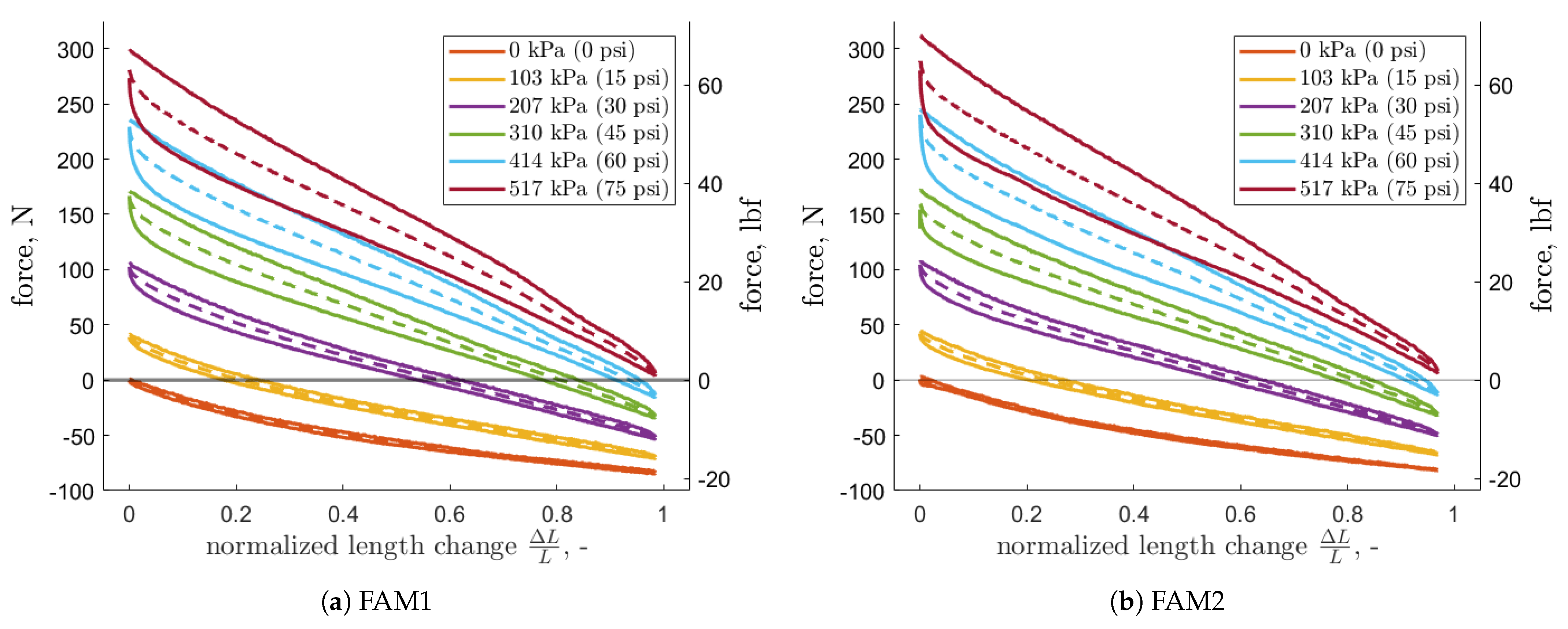
The obtained static force responses are plotted in
Figure 6. FAMs produce blocked forces that linearly increase with pressure, which is the same trend that was observed for CFAMs [
9,
33,
34]. The forces are approximately ten times smaller than those of contractile FAMs with a similar resting diameter, which agrees with Pillsbury et al. (2017) [
9]. The EFAMs tested here have slightly larger blocked forces than those previously tested in [
9]. The higher blocked forces are likely a result of the manufacturing method which keeps the braided sleeve tight on the bladder (as compared to the method with excess braid, which results in a gap between the bladder and the sleeve). The fabrication method described in
Section 2 also resulted in improved free extension. For a comparable pressure value of
kPa, the free extension is more than two times larger than that reported by Pillsbury [
9] and
times larger than that reported by Trivedi et al. [
43]. The EFAM design used here improves blocked force and free extension, and may feature good fatigue properties similar to those of the CFAMs [
3].
4. Modeling
In this section, the EFAM static force response is modeled together with estimation of the bladder’s hyper-elastic behavior. The analysis performed in this section validates an existing modeling technique for use with EFAMs, gives insights about estimation of variables and constants that appear in the model, and proposes a new modeling approach to account for bladder elasticity.
The literature on FAM modeling is extensive, focusing on two main modeling approaches: energy [
30] and force balance models [
13,
33,
34]. The force-balance model (Equation (
2)) was employed here, as it was shown that this model makes no assumption on the value of FAM’s resting braid angle. Thus, Equation (
2) can be used to model contractile and extensile FAMs [
9].
The variables in the equation are FAM’s axial force,
F, internal pressure,
P, dead-band pressure,
, number of braid thread turns,
N, specimen length,
L, length of a braid thread,
B, longitudinal and circumferential stress,
and
, bladder material volume,
, bladder thickness,
, and the FAM’s outer radius
. With
and
being functions of FAM’s length, and stresses
and
being typically functions of
L and
P [
9], we get an equation fully defined by force, pressure, length, and constants.
In the force-balance model, FAM geometry is constrained by its design and by assumptions that simplify the analysis. The thread of the braided sleeve is assumed to be constant length and inextensible with a negligibly small diameter. The bladder is modeled as a thick-walled cylinder (
Figure 2b) with a constant volume by the assumption that the bladder material is incompressible. Although the authors find this model sufficient for the performed analysis, there are improvements that can be implemented such as: relaxing assumptions on the braid thread inextensibility and bladder incompressibility, introducing a non-cylindrical FAM shape at the ends [
34], extending the model with braid-bladder friction [
30], or including temperature and time-dependent mechanical effects in
and
.
4.1. Resting Braid Angle Estimation from Geometric Properties
The assumptions and resulting geometric constraints introduce a set of constants that are needed for modeling. In Equation (
2),
B is the length of the inextensible braid threads. Its value can be calculated from measurable quantities when the FAM is in its resting state:
where
is the resting working length of the FAM and
is the resting braid angle. As direct measurement of the angle is problematic (
Section 2), the braid angle was obtained with the following calculation. The number of turns
N is always constant and given by the equation [
34]:
which leads us to a formula for the resting braid angle:
that uses constants that were obtained during the fabrication process such as the braided sleeve diameter,
, the braided sleeve length measured,
(where the subscript indicates that both variables should be measured at the braid angle of 45 degrees), EFAM resting length,
, and EFAM outer resting diameter,
. For an EFAM with a rolled-up sleeve, this value is theoretical, as the excessive amount of sleeve gives the braid angle lots of freedom to change over the length of the sleeve (see
Figure 4). The braid angle is then used to compute the number of turns,
N.
4.2. Working Volume Estimation
The next constant is the bladder volume,
, which was estimated based on the pre-assembly geometrics of the elastomeric bladder. The bladder length, fixed by the end fitting, will not equal its mounting channel length because the channel has different dimensions than the elastomeric tube. The bladder was assumed to be incompressible, and therefore the excess volume of a part of the elastomer would be pushed outside of the end fitting channel. By considering the volume of the channel, the amount of the working bladder length that is lost in the swaged end fittings can be calculated.
where
is the volume of the bladder clamping channel modeled as a thick-walled cylinder, which is defined by its length,
, (times two for both end fittings) and radius,
. The sub-subscript
denotes the inner radius of the channel, and
denotes the outer radius of the channel. The braid thickness is denoted as
.
, can be used to calculate how much of working bladder length
was lost to fix the bladder in the end fitting. Then, the working bladder volume can be calculated as follows:
where the inner radius of the bladder is denoted as
, the outer radius of the bladder is denoted as
and the original bladder length is denoted as
. In the case of the studied extensile FAMs, where
cm, if there were no deformations, the working bladder length would be
cm. The deformations during fabrication and cycling change the resting length and outer diameter. For FAM1 the resting length is
larger and for FAM2,
larger. The resting diameter was
larger for both FAMs than that of off-the-shelf latex tubes. The working bladder volume for the tested FAMs was found to be
liters.
4.3. Dead-Band Pressure Estimation
Dead-band pressure,
, is the pressure required for the bladder to make substantial contact with the surrounding braid and initiate inflation of the FAM [
16,
30,
34,
44,
45]. The dead-band pressure was measured experimentally. According to the Gaylord model, the blocked force is linearly proportional to FAM’s internal pressure, and equals zero when pressure is not applied. This is not the case with the experimental data. A linear fit to the experimental data in
Figure 7a would yield a pressure value greater than zero for the blocked force of zero—a pressure level above which a FAM starts to generate force. This pressure difference between the Gaylord model and the experimental data is the estimated value of the dead-band pressure.
The Gaylord force model [
4] considerably overestimates the force of contractile FAMs; however it was found to be accurate for estimation of FAM blocked forces [
9,
33], which makes it also useful for dead-band pressure and resting braid angle estimation. Additionally, it can also be shown that the Equation (
2) for blocked force conditions is equivalent to Gaylord’s equation:
where the resting braid angle was denoted as
, the resting outer diameter as
, the FAM internal pressure as
P, and the dead-band pressure as
. The blocked force,
, in the experimental data was observed to have a strong linear trend (
Figure 7a), which is justified by Equation (
9). With a linear fit, dead-band pressure,
, is obtained where
. For the two FAMs, the estimated dead-band pressures are
kPa and
kPa, as compared to
kPa that was used by Pillsbury et al. (2017) [
9] where the bladder material was also latex, the bladder had the same thickness and the same or even larger diameter. It is worth noting that larger dead-band pressure probably led to a smaller blocked force observed in their study for extensile FAMs.
4.4. Resting Braid Angle Estimation from Experimental Data
The previous method for estimation of the resting braid angle used only geometric properties of the bladder, the braided sleeve and the end fittings. This allowed for calculation of the braid angle prior to experimental characterization. To validate the previous method, another method based on the experimental blocked force data is introduced to validate the previous one. For the experimental method, blocked forces and dead-band pressure values can be used to estimate resting braid angle, . The method is very sensitive to the measured resting diameter as the blocked force is proportional to the square of the outer diameter, . Since there is a variation in the measured resting outer diameter, the authors decided to pick a value from the range that would give a reasonable fit. For both FAMs, the resting outer diameter, , of cm was found to agree well both with the experimental data and the previously estimated braid angle. This resting diameter value is therefore used throughout the rest of this work.
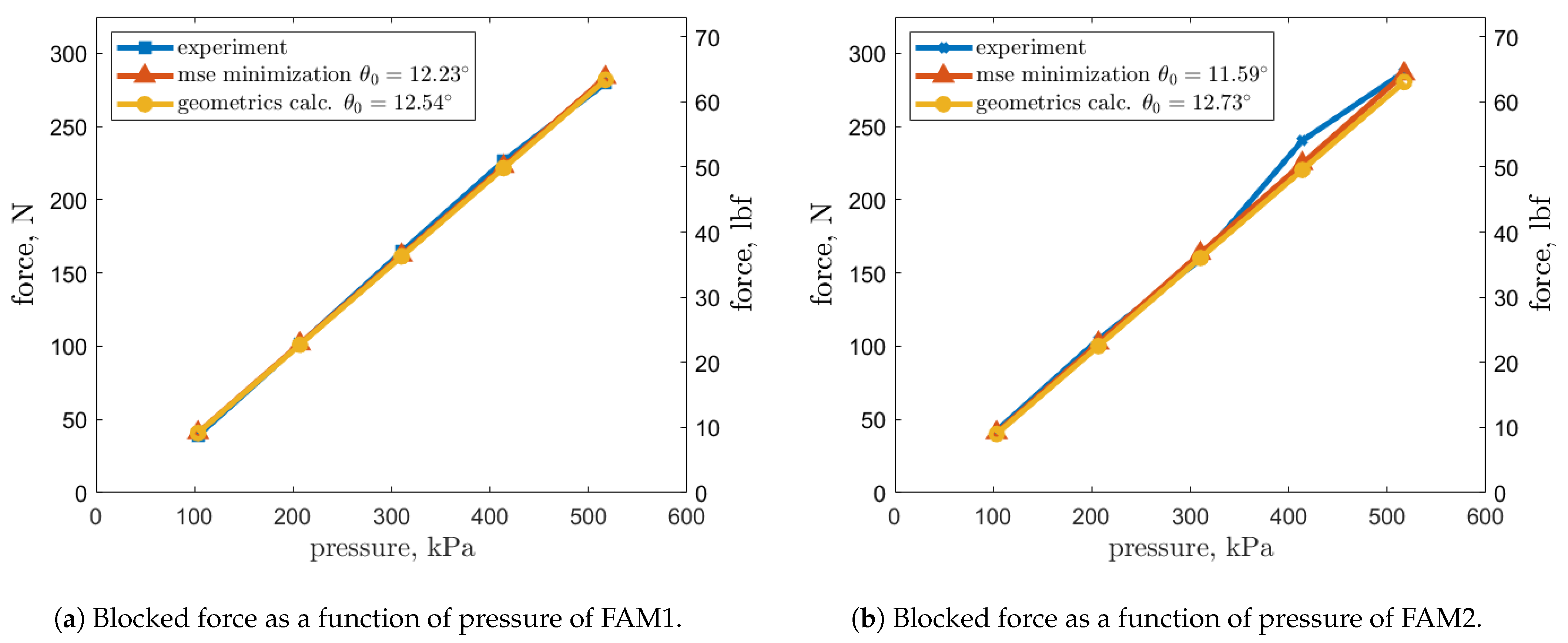
A mean squared error function can be devised and used with a non-linear programming solver such as MATLAB
®’s fminsearch to find a braid angle that matches the blocked force data with Gaylord’s force model (
Figure 8). The experimental values that do not follow the linear trend of Gaylord’s model are treated as outliers. Alternatively, an average value of the tangent of resting braid angle
can also be obtained from data when one isolates
from Gaylord’s model. It was found that the first experimental method was simpler to implement, and chose it because it directly minimizes the error, that depends on the braid angle, between Gaylord’s model and the experimental data on blocked forces. Blocked force value for FAM2 at a test pressure of
kPa does not follow the trend and was treated as an outlier.
The changes for the braid angles found through minimization of the error between the model and the data, compared to the values from the geometric method for the resting braid angle,
, of
° and
°, were
and
for FAM1 and FAM2 accordingly. The small differences in the estimated resting braid angles, and the small error between the blocked force values shown in
Figure 8a,b validate both methods for braid angle estimation. The method based on geometric measurements gives the advantage of blocked force estimation prior to the experiment. Thus, it allows for accurate predictions of EFAM braid angle with simple measurements. With additional studies of differently sized FAMs, one could show bounds on the bladder’s resting length and diameter change due to manufacturing and cycling. This would allow for even more precise blocked force estimates at the design stage. Braid angles based on geometric properties of
° and
°, were used for later analysis.
4.5. Calculation of FAM Outer Radius and Bladder Thickness
Variables such as generated force,
F, FAM length,
L, and internal pressure,
P, were assumed to be given or measured by the testing system. Since
B,
L, and
N are known and the assumed thick-walled-cylinder shape of the FAM fully defines the geometry, the FAM outer radius
(which is here assumed to be equivalent to the braided sleeve radius) can be calculated as follows [
33,
34]:
where the length of a sleeve thread is denoted as
B, FAM length as
L, and number of thread turns as
N. The bladder thickness,
, may be then obtained with [
33,
34]:
4.6. Numerical Estimation of Bladder Material Stress Function
Modeling the stress as if the bladder were a thick-walled tube of linearly elastic material yields good results (the blocked force was predicted within
of the experimental measurements) [
33]; however, the hyper-elastic model using a polynomial form allowed for a practical model with smaller error. Originally, the proposed hyper-elastic model by Hocking was composed by fitting coefficients to each force response curve at different pressures [
34]. The studied axial force responses revealed that the material stress was moderately linear to the operating pressure—an observation used in this study. Unlike Hocking, who studied contractile FAMs, this study covers extensile FAMs, and so modeling methods and observations previously used for CFAMs should be re-validated for EFAMs.
So far, all of the variables and constants in Equation (
2) were covered besides material stresses. The two stress terms: longitudinal bladder stress,
, and circumferential bladder stress,
are functions of strain,
, and, since the material behavior changes with pressure [
37], internal pressure
P. The longitudinal stress is dependent on longitudinal strain,
:
and the circumferential stress is dependent on circumferential strain,
, that is calculated with the cross-sectional center of the bladder to includes the variation of the bladder thickness [
33]:
The final component to the Equation (
2) is the bladder stress function
. If a form of such a function was known and it had some coefficients defining the properties of the bladder material, then it would be possible to search for the coefficient values, comparing the axial force of the force-balance model (Equation (
2)) with the axial-force experimental data. Then, numerical methods such as nonlinear programming solver could be used to find coefficient values that give the minimum error. This coefficient search method was employed in this study. For error minimization, the normalized force error is summed at a number,
n, of uniformly distributed normalized length changes, averaged with division by
n, and then summed for each pressure to be then averaged by division of the number of different test pressures,
. Model coefficients for the stress functions are determined using fminsearch in MATLAB, the axial-force-response experimental data, and the error cost function:
where
is the number of test pressures (in this study,
and
). In the Equation (
14),
denotes the force measured by the testing system,
denotes the force calculated with a model. The subscript,
, denotes length change at which the force values were acquired. The superscript,
indicates the internal pressure at which a given test was performed.
The Nedler–Mead algorithm (fminsearch) was chosen for its simplicity and its familiarity to the first author [
46]. MathWork’s fminsearch implements a Nedler–Mead algorithm that starts at one set of initial values. Use of other algorithms that have more starting points, or simply using a multi-start version of fminsearch might increase a likelihood of finding a better local minima. Two groups of such algorithms are evolutionary and swarm algorithms used in population-based optimization methods [
47]. For this problem, MATLAB’s genetic algorithm,
ga, was also tried instead of fminsearch, but surprisingly, it yielded errors that were three times larger in value than the ones that were obtained with fminsearch.
It is hypothesized that the more important factor for this problem was picking a “good enough” starting point for fminsearch or “good enough” bounds on coefficients for the genetic algorithm. In this study, an elastic model was used for a baseline, and was described further in the next section. That baseline model used only two coefficients which made the search simple. With our other models, non-linear terms were added to the baseline model with an aim to improve the regions of transient behavior for small, or large strains. The non-linear terms extended the search to four coefficients. Since the new models were an extension of the baseline model, the coefficient values found with the baseline could be reused as starting points for the new models. As can also be seen in the following section, for certain models, one can find bounds on the coefficients, which makes it even easier to find a good starting point for fminsearch, or narrow the search space when using another algorithm such as genetic algorithm.
4.7. Stress Function Model Structures
To identify the parameters, the form of the stress function, , is first needed. Since the latex-rubber bladder stress response to strain and pressure can vary with factors like time, temperature, UV light or humidity, a pressure-dependent hyper-elastic behavior of the EFAM bladder is not fully known. In this section, four different stress function are evaluated for modeling of this subtle EFAM bladder behavior. All models include a linear term and use four parameters that are the output of fminsearch. With iterative testing, four appears to be the smallest number of parameters that provides sufficient degrees of freedom for a good fit of the stress function to measured data.
Four stress functions were selected to represent four different approaches to hyper-elasticity. The stress functions let us gain physical insights from the trends of various parameters. A linear stress function was selected as the baseline, and the three other stress functions added higher order hyper-elastic terms to the linear model.
The first stress function, denoted as the linear model, assumes a linear elastic bladder with stiffness linearly dependent on pressure [
33]:
where
refers to the coefficients obtained by the minimization algorithm.
is an equivalent of Young’s modulus for rubber, and was expected to be positive and range from 1 to 5 MPa.
was used to model the pressure effect, which was assumed to be linearly increasing [
33]. Given that the two parameters were positive and thus the positive strain derivative of stress was also positive,
, the material stability of the linear term was guaranteed with
and
.
The second stress function, denoted as the polynomial model, assumes hyper-elastic material with a 3rd order polynomial stress–strain relationship. This form was chosen based [
9] as it successfully modeled both, CFAMs and EFAMs. The order of the polynomial expression was chosen through trial and error.
The stability of this material model can be analyzed with its stress–strain derivative:
Since the linear term was shown to be positive, a constraint is introduced to guarantee material stability:
The constraint adds complexity to the non-linear optimization procedures, which based on authors’ experience may lead to the end optimization at local minima that do not give a good fit. This was even more apparent for polynomial models of higher orders that were not included in this study. As shown later in the results, for a good fit, should be negative, which runs counter to the idea of using a simple constraint where all the coefficients are assumed to be positive.
The third and fourth stress functions evaluated here were inspired by tensile stress–strain relationships found for rubber in Treloar’s (1944) [
38] work on vulcanized data. The added terms were chosen to directly address the non-linear effects in rubber-like materials. The third stress function, denoted as the exponential-decay model, uses an exponential term with the goal of modeling initial “transient” state for small strains which was observed in the data.
The stress–strain derivative of the exponential-decay model is:
Since was used for scaling of the non-linear term, and becomes an added linear term when , it was explicitly assumed to be positive. Additionally, the sum of and should give a value close to that of from the linear model. For the exponential term to vanish, must also be positive. With these two simple requirements, the stress–strain derivative is also positive, which makes the material model always preserve Drucker’s stability.
The fourth stress function, or the exponent model, was inspired by Ogden’s (1972) [
36] work. It is composed of terms with increasing and decreasing derivatives, which was obtained by constraining
and
. The goal of the
was to model the transient effect for the small strains, and
was to model strain stiffening. The parameter,
, appearing in all models, was here reused for scaling of the exponential terms.
The stress–strain derivative of the exponent model is:
With and being positive values, the strain derivative of stress is guaranteed to be positive at all times which guarantees material stability. Note that for negative strains, the strain terms, , need to be substituted with to avoid imaginary values.
More variations of function structures can be studied, and many of them may need fewer coefficients, or provide smaller errors. However, the important aspect of the two proposed function structures is that the non-linear effects of choice can be added through related terms; the function shape is based on and constrained to physical behavior; and that they guarantee material stability. Although polynomial expressions are often used to model non-linear behaviors, their structure may leave out degrees of freedom, which based on experimental data, or elastic material models are unrealizable by rubber-like materials. Leaving out additional degrees of freedom for the optimization procedure, or introducing complex constraints, might lead to the optimization process converging at a local minima that give an undesirably large error. One could also consider modeling the non-linear behavior with terms such as sigmoid or arccotangent functions. They could potentially give lower errors, or fit the small strain transients better. However, for this study, the emphasis was made on selecting terms that were considered simple and providing physical insight.
4.8. Modeling Results
The maximum normalized length change was divided into five points,
, and the error was computed for each point. Then, the sum of the errors was taken and normalized by the number of evaluated points and another sum was taken over a number of pressure tests,
, as listed in Equation (
14). The sum was then divided by
. Compared results were shown in
Table 3 and optimization results in
Table 4. The introduced constitutive models (Fun (
19) and (
21)) were characterized by smaller errors than the previously-used models (Fun (
15) and (
16)). In this study, the polynomial model (Fun (
16)) reached a similar average error to exponential-decay model (Fun (
19)) and exponent model (Fun (
21)). Only 5% improvement was shown, compared to the polynomial model.
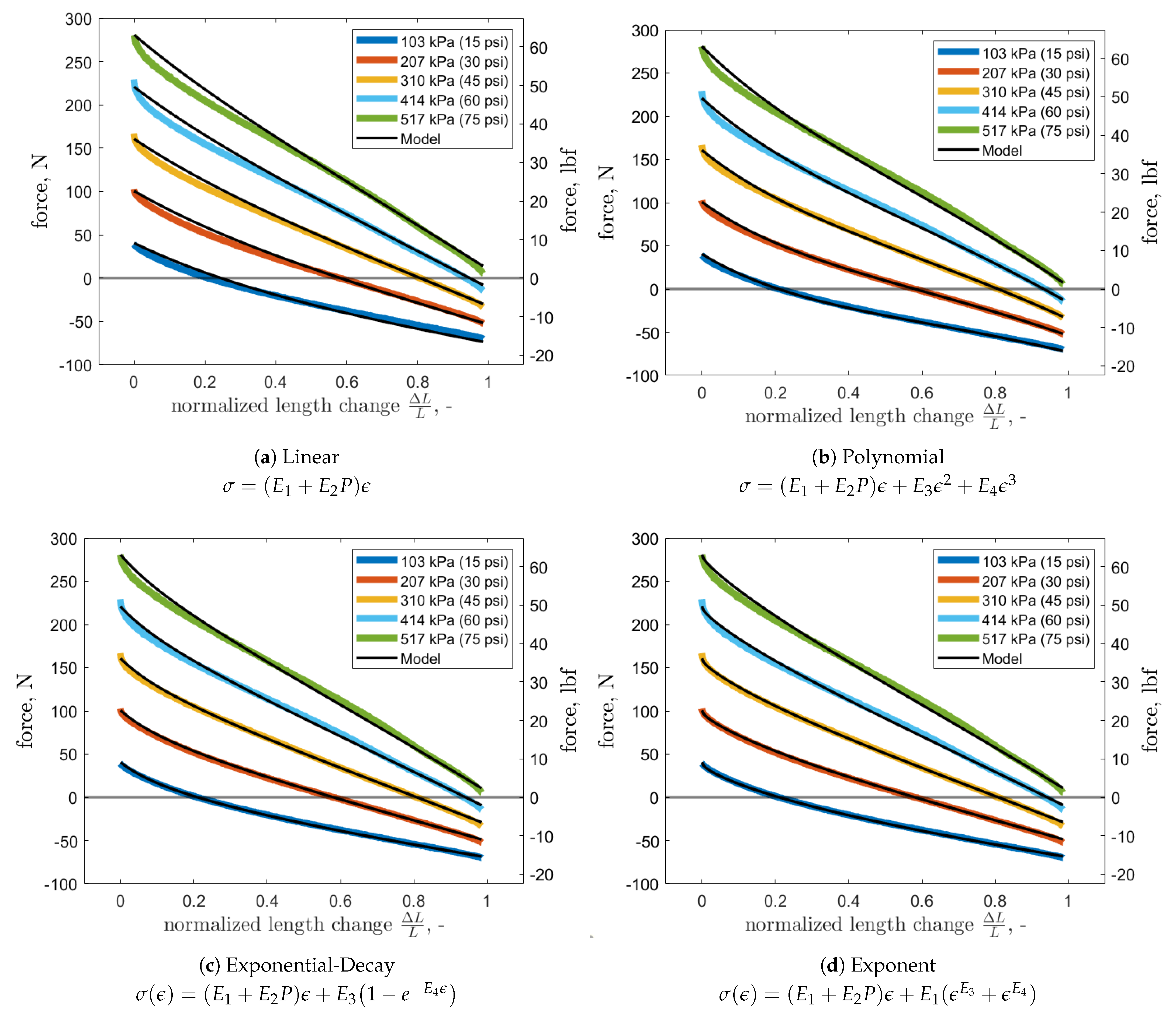
In
Figure 9, four subfigures show the same axial force response of FAM1 with an overlaid black curve representing results obtained from modeling of the axial behavior with a given stress function structure. Although in
Figure 9a the linear model gave a satisfactory fit, it failed to model the non-linear behavior for small strains. For free extensions the fit starts to deviate for larger internal pressure levels, although for the testing pressure range it still gives a good fit. For all other stress function structures, the model fits the free extensions precisely. At the cost of additional coefficients in
Figure 9b, the polynomial model provides a better fit for small strains that worsens with increasing FAM internal pressure. The two new proposed stress functions model the small strain region slightly better than the polynomial model. From an engineering perspective, all the models match the data well, with the hyper-elastic ones mainly introducing improvements in the small strain region, which might be of importance for precise actuation. The qualitative observations were confirmed for FAM2 (
Figure 10), and further validated quantitatively in
Table 3.
For FAM1, the stress function for strain up to 10% and up to 400% was plotted to show comparison between the modeled stress functions.
Figure 11a shows how different models captured the transient state for small strains. The polynomial model did not capture the transient state and the proposed models did, which can be further observed in the modeled axial force response in
Figure 9b and
Figure 10b.
Figure 11b shows stress values for strains outside of the testing range. For large strains, the polynomial model can yield behavior that is unrealistic. Here, it quickly exceeds realistic stresses for rubber, which makes it impractical for predictions of non-measured strains.
The exponential-decay model yields an almost linear increase in stress for large strains, which is beneficial if one needs a conservative model outside of a tested strain region. Although the exponent model assumes exponential increase in stress, the modeling-error minimization was able to “learn the stress behavior”, which resulted in stress increasing only slightly faster than that of the linear model for large strains.
A high-level comparison of the stress models is shown in
Table 5. The average error was calculated from the average errors for the two FAMs shown in
Table 3. Expanding the linear model with non-linear terms led to a decrease of the average error by 50%. Among the three non-linear models, the exponent model had the smallest average error.
Next in
Table 5, complexity of the conditions for material stability were compared. For polynomial model, an inequality with different coefficients was needed to satisfy material stability. For all the other models, one-coefficient inequalities were needed to be evaluated, which simplified material stability analysis and optimization procedures.
Next, the models were compared with their growth rates using Big O notation. Growth rates were found to quantify how conservative the models would be outside of the tested range of strains. If the growth rate is big, as was the case with the polynomial model, then the model might give physically unrealistic predictions of stress outside of the tested region. The most conservative were the linear and exponential-decay models. Since in the exponent model
, its growth rate comes from
. Theoretically, this gives the model a potential to become unrealistic for large non-tested strains; however, in the case of this study,
for FAM1 and FAM2 was
and
respectively. The polynomial model has
, which gives the model a fast growth rate, and can lead to a quick stress increase as was shown in
Figure 11b.
For finding the coefficients through optimization, it is important to know what the bounds on the coefficients are. This was summarized in the last column
Table 5. For the linear model, the bounds on
are known from empirical data on rubber-like material properties.
has to be positive for every model as it was discussed in
Section 4.6, which means that the lower bound is known. For the polynomial and exponent model, bounds on
are not explicitly known because other terms affect the total stress values. For polynomial model, the bounds of other coefficients are also unknown as the coefficients do not explicitly link to non-linear effects.
Since the exponential-decay model becomes approximately linear after the exponential term vanishes, it inherits bounds from the linear model and has an upper bound on as it is a fraction of linear model’s . As is an equivalent of the multiplicative inverse of a time constant, , of a stable first order LTI system, it has to be positive. The analogy to the time constant also sheds some light on when the small-strain non-linear effect vanishes. After the time of 3 time-constants, the term, , is , which is here defined as a point after which the non-linear effect becomes negligible. This means that the non-linear effect vanishes at strains of 23% and 10%, for FAM1 and FAM2 respectively.
For the exponent model, coefficient has a lower and an upper bound and coefficient has a lower bound based on the model’s definition. The linear model was the model for which the most was known about its coefficient values because of its simplicity. Among the non-linear models, however, it was the exponential-decay model that gave not only the largest number of bounds, but also the bounds that were connected to the physical behavior.
5. Discussion
Little was found in the literature on differences between contractile and extensile FAMs in manufacturing, testing and modeling as few studies dedicated specifically to EFAMs were found. The first question in this study sought to determine whether the methods developed for CFAMs can be adapted for use with EFAMs.
The loose sleeve on the elastomeric bladder makes braid length measurement methods of CFAMs impractical for use with EFAMs. Two methods for braid angle estimation have been shown (see
Figure 8). The first method is based on the design variables and geometrical measurements, and the second is based on the experimental characterization of the muscles. Relative to the first method, the second method showed that the differences between the braid angle values for the specimen were
% and
%, accordingly. This validated the design-based braid angle estimation method, which was found to be useful for calculations prior to experimental characterization.
Since the EFAM resting diameters changed after initial cycling, calculating a bladder working volume from post-cycling measurements was found to be inaccurate. A method that included an effect of a clamping mechanism on the bladder was used and based off pre-assembly measurements. After initial cycling of the two specimens, an increase of and in resting lengths and for the resting diameters were observed. Although the study did not aim to examine this effect, the measured geometrical changes were found to strongly affect the modeling results. The modeled axial force response is especially dependent on the resting diameter, as the FAM axial force is proportional to the square to diameter’s value.
Dead-band pressure was found to be smaller than those obtained for a comparable EFAM in a previous study [
9]. This was attributed to the tighter fitting between the bladder and the sleeve during manufacturing process. And, as can be seen from Equation (
9), a lower dead-band pressure increases the blocked force of an EFAM.
One interesting finding is that the experimental data have relatively large hysteresis when compared to the previous studies on CFAMs (
Figure 6). It is hypothesized that the difference in hysteresis might come from the friction between the plastic tube that prevented the specimens from buckling and the braided sleeve. This hypothesis would agree with the size of the hysteresis decreasing with decreasing FAM internal pressure and decreasing with increasing length of the EFAM. At low internal pressure, the force acting on EFAM walls is smaller as with increased length the braid kinematics force the EFAM outer diameter to reduce its size, relieving the anti-buckling tube. In a future study, one could design an experimental version of an EFAM that would be constrained from buckling with an internal rod rather than with an external tube. The hysteresis in such case could be simpler to quantify and more readily attributed to the bladder hysteretic behavior.
In
Figure 7a, an outlier point in the data was observed for FAM2. The source of that deviation from a linear trend remains unknown. In
Figure 7b, it can be seen that the EFAM reached an extension close to
, a value which has not been reported in the literature covered by this study. Both results might indicate that the design was improved from previous studies as the FAMs also provided a blocked force of approximately 280 N and a large maximum stroke of 98% at 517 kPa, and low dead-band pressure of 35 kPa. All values indicate a better performance than that of a comparable EFAM tested in Pillsbury et al. (2017) [
9]. However, it should be noted that temperature may have differed during the various tests under comparison, which may have lead to variability in bladder properties.
The study also focused on modeling of the bladder constitutive model non-linear terms, because models other than polynomial could provide better fit to data, satisfy material stability criterion, ease parameter identification. All of the hyper-elastic constitutive models showed nominal errors of 2%, while having the same number of coefficients.
Although the polynomial model uses the same number of coefficients as the other non-linear models and has a similar error, the process to obtain its final form proved to be difficult. Following tests with different forms to minimize the number of coefficients, a polynomial model was found, but there are no implications that this form would also work for different types of FAMs. Moreover,
Figure 11b shows that outside of the tested strain region, the stress rises quickly and gives values that greatly exceed stresses reported for rubber [
38], rendering the usefulness of the polynomial model outside of the tested region questionable.
The exponential-decay model and exponent model yielded only positive coefficients which fulfilled Drucker’s material stability criterion [
40] without further analysis. The exponential-decay model is the most conservative about predictions of stress–strain relationships for untested strain values. For larger strains, the exponential term vanishes, and the model assumes a nearly linear relationship outside of strains that are not in the range of experiments. The drawback of the exponential term in the exponential-decay model is that for larger strains, the form is not capable of modeling the strain-stiffening effect as the decaying exponential term can only model the initial “transient” state. The Ogden-inspired exponent model, however, can model the stiffening and has small discrepancies between the coefficients for the two tested EFAMs, which gives it an advantage over the exponential-decay model. On the other hand, the exponential-decay model has a broader set of defined bounds on its coefficient, which is advantageous when identifying parameters of the stress function.
6. Conclusions
In this investigation, the primary aim was to introduce new hyper-elastic constitutive models and revalidate methods for extensile FAMs (EFAMs) that were previously studied for contractile FAMs (CFAMs). The secondary aim of the study was to investigate manufacturing process, measurements, and experimental characterization of EFAMs as they were adapted from more extensive studies of CFAMs.
Four constitutive models of an elastomeric bladder were investigated to gain physical insights into the bladder’s behavior. An elastic model, the linear model, was chosen as the baseline. The other models were formed as an extension of a pressure-dependent elastic model, the linear model, with hyper-elastic terms. The polynomial model was chosen to represent a previously investigated approach in the literature. The exponent model was inspired by the work of Ogden (1972) [
36]. The exponential-decay model with a vanishing non-linear term, was selected based on experimental data showing an initial “transient” state for small strains. As shown in
Table 5, all studied hyper-elastic constitutive models showed relatively small errors of around 2% as compared to
% of the elastic model. The linear, exponent, and exponential-decay models required simple one-coefficient inequalities to check for Drucker’s material stability [
40] as compared to multi-coefficient inequalities for the polynomial model. Since hyper-elastic behavior for large strains of the bladder might be not known, a conservative model for untested strains was considered advantageous. Among the hyper-elastic models, the exponential-decay model had the most conservative growth rate of
as compared to polynomial-order or coefficient-dependent growth rates of:
and
for the polynomial model and exponent model, respectively. In order to identify stress function parameters, it was important to assess bounds on the model coefficients, as listed in
Table 5. For the polynomial model, only one parameter had a lower bound. The exponent model and the exponential-decay model had bounds or simple bounds on every coefficient, as listed in
Table 5.
The results revealed that for the modeling of a non-linear bladder behavior with the force-balance model, it is beneficial to use the newly introduced exponential-decay model. The model was shown to have the advantage of small error when compared to other models, well-defined boundaries on constitutive model coefficients, and simple conditions for meeting Drucker’s stability criterion. The model was also found to be conservative outside of the range of measured strains, as it converges to a linear model as the strain growths. Moreover, it allows for finding the range of strains influenced by the transient behavior.
Primarily, the findings of this research provide insights into selecting an EFAM bladder constitutive model. Secondarily, the study revalidated and adapted methods previously studied for CFAMs in the EFAMs context. Thus, the insights gained from this study can inform research in the field of soft robotics, with a particular focus on EFAM-driven continuum soft robots.
The current study is not without limitations. The findings are not generalizable as only two EFAMs of the same size and materials were experimentally tested. Another limitation is that the parameter optimization relies on initial guesses of the model parameters. Moreover, the hysteretic behavior observed in the experimental data was not addressed. Finally, an additional uncontrolled factor was the temperature under which the experimental characterization was conducted.


