1. Introduction
The development of control systems and deployment on an embedded electronic control unit (ECU) is a complex task supported by several complex software tools. In general, a differential equation-based mathematical high-fidelity model describing the dynamics of the system to be controlled offers a valuable starting point for the development of a model-based control system [
1]. Deriving, transforming, and discretizing the ordinary differential equations (ODEs) or differential algebraic equations (DAEs) of the system dynamics directly from the first principals of physics is a nontrivial, tedious, and error-prone task [
2].
To facilitate the modeling process, several multi-domain modeling languages (e.g., Modelica, VHDL-AMS, Simscape, Modia) were developed in the past [
2]. These languages allow the user to define high-level models across different domains (e.g., mechanics, hydraulics, electrics). Usually, the system to be controlled as well as the control system can be composed of the predeveloped components provided by a wide range of system libraries. To emphasize the composition of different physical domains in one simulation model, we will refer to these kinds of models as multi-physical models in the following. Assembling multi-physical system models out of existing and validated model libraries speeds up the modeling process, minimizes modeling errors, and allows the creation of highly complex high-fidelity models of the system to be controlled.
In the case that the existing model libraries are not sufficient, new components can easily be implemented. The acausal characteristic of those modeling languages allows the user to implement the system dynamics of new components as DAEs. In these modeling languages, the transformation and discretization of the equations are automatized, speeding up the development of new components and reducing errors which might occur during the manual transformation of the equations.
Further advantages of developing and optimizing control systems in high-level modeling languages like Modelica [
3] can be summarized as follows: The availability of high-fidelity system models provides the possibility of testing and optimizing the control system during an early phase of development. Moreover, high-level modeling languages, such as Modelica, allow the integration of detailed system models into the control system. This is especially useful for methods based on inverse models [
4] or nonlinear Kalman filter methods [
5]. In addition, nonlinear MPC methods require a physical model of the plant [
6].
To deploy and execute control systems based on multi-physical models on embedded ECUs, the control system must be transformed to a low-level programming language (usually C) and then compiled for the specific embedded target. This can be achieved by manually reimplementing the control system in the desired programming language or by automated code export [
7]. Manual transformation is tedious, error-prone, and requires profound knowledge of different disciplines. Therefore, efficient automated code export is desirable.
One method to generate C code from high-level modeling tools is the use of Functional Mock-up Units (FMUs), which contain the model as source code. Although it has been shown that it is possible to use C code generated by FMU export for embedded targets [
8], several weaknesses have been identified. The FMI Standard [
9] was developed to unify the exchange and coupling of dynamic system models between different simulation environments on personal computers (PCs). Since the FMI Standard was not designed for execution on embedded targets, important properties like traceability of code, information about the used compilers and compiler settings to ensure repeatability, the handling of limited memory, and computational power or real-time capability were not considered [
10].
The desire for a continuous toolchain to support the design and deployment process of model-based control systems on embedded targets motivated the development of the eFMI Standard (Functional Mock-Up Interface for embedded systems) [
10,
11]. In contrast to the known FMU, “an FMU for embedded systems (eFMU) is a shared development workspace for step-wise, semi- and full-automatized refinement from a high-level intermediate representation of a sampled algorithm […] to an implementation of the algorithm for an embedded target” [
10] (p. 59). Additionally, the eFMI Standard describes the so-called eFMI workflow. This workflow summarizes a set of steps which must be performed to successfully deploy a control system—designed in a high-level modeling language—on an embedded target utilizing eFMUs. Although some contributions (such as [
10]) discuss the development of the eFMI Standard co-developed by the authors, a comprehensive application and verification study of the new standard in scope of a typical control design problem is currently missing. This includes the handling of typical requirements for industrial applications as well as the integration of state estimators, such as Kalman filters, for the controller development based on eFMI.
Thus, the goal of this work is the utilization, implementation, and verification of the eFMI workflow. For this purpose, the application to the automotive vertical dynamics control problem is selected. We demonstrate the integration of the eFMI workflow into the controller design process aided by high-level modeling tools. Furthermore, we discuss the different steps which are necessary to successfully develop, export, validate, deploy, and execute a model-based controller as well as a nonlinear Kalman filter on a low-volume production ECU. Hereby, we explain additional steps which are necessary to integrate an eFMU into an embedded Kalman filter library. We utilize different test configurations to validate the different transformation steps defined by the eFMI workflow and performed by tool prototypes. In the application of the eFMI workflow we integrate two different eFMUs into the software framework of a single ECU, one as a prediction model for a nonlinear Kalman filter and one as part of a model-based vertical dynamics controller.
The novelty of our approach lies in having automatically derived an embedded software solution from a high-level multi-physical model with standardized eFMI methodology and tooling. We present one of the first full application scenarios—covering all aspects of multi-physical modeling and embedded target deployment—of the new eFMI tooling.
The paper is organized as follows: In
Section 2 the automotive vertical dynamics problem is introduced.
Section 3 describes the eFMI workflow and the different model representations specified by the eFMI Standard. Subsequently, in
Section 4 the application of the eFMI workflow to the automotive vertical dynamics control problem, including modeling, controller design, eFMU generation, eFMU integration, and deployment, is described and discussed.
Section 5 presents the results of offline tests, which were conducted to validate the toolchain. Additionally, the outcome of the online tests carried out on a series-production car are discussed. Finally,
Section 6 summarizes the work and provides an outlook.
2. The Vertical Dynamics Control Problem
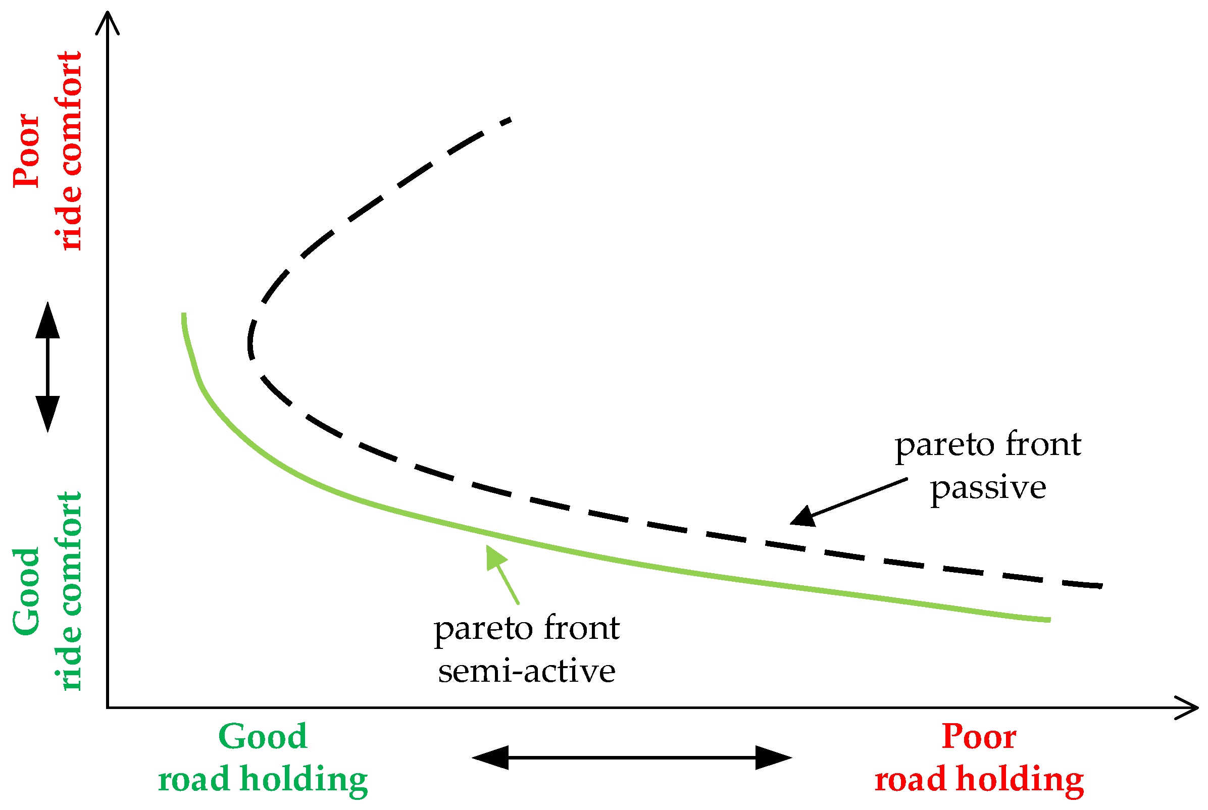
In automotive applications, the goal of vertical dynamics design is to optimize the vehicle chassis suspension such that certain objectives are fulfilled. The main objective is the concurrent maximization of ride comfort for the vehicle passengers and road holding of the tires. Optimizing the former criterion yields an increase in passenger comfort, thus enhancing the driving experience. In contrast, the optimization of road holding contributes to the safe operation of the vehicle. Since all the necessary forces for vehicle guidance are provided through the tire-to-road contact patch, the condition of road contact is significant for vehicle safety, especially in critical driving situations.
Although ride comfort is a complex and highly individual metric, suitable simplifications allow to assume that a reduction of the comfort criterion is achieved by minimizing the vehicle chassis acceleration [
12]. Like the quantification of the ride comfort, the modeling of tire–road contact is a complex task. Nevertheless, the following valid assumption holds: The greater the normal force on the tire, the greater the admissible lateral and longitudinal tire forces. Thus, the road holding criterion generally aims at maximizing the tire normal force. This force is composed of a static and a dynamic part. The static part originates from the body mass and the tire mass, as well as gravitation. Since these quantities remain constant during operation, the goal is to optimize the dynamic tire force. If only stochastic road excitation with zero mean is assumed, the integral of the dynamic tire normal force over all time is zero [
13]. As a result, improving the dynamic tire force at one point in time reduces the tire force at another time. Consequently, the road holding criterion is often reduced to minimize the norm of the dynamic tire force over all time.
As shown in [
12] these two objectives are partially contradicting.
Figure 1 shows that changing the suspension setup only can improve one objective to a certain degree without having a negative impact on the other. At this point, semi-active dampers offer the potential to improve the trade-off between road holding and ride comfort as compared to passive systems.
A common approach to changing the semi-active dampers’ characteristics is to either control the oil flow through a valve or to adapt the viscosity of the fluid directly through electrorheological or magnetorheological effects [
12].
Figure 1 shows that by choosing an appropriate control system for the semi-active damper, a better trade-off with respect to road holding and ride comfort is achieved.
The vertical dynamics controller must compensate for two kinds of excitations: driver-induced disturbances and road-induced disturbances. Driver-induced disturbances originate from the steering, braking, and acceleration actions of the driver and mainly induce a pitch and roll movement of the vehicle. Since there is a significant time delay between these actions and the resulting longitudinal and lateral accelerations, the effect of the driver-induced disturbance can be well predicted. In contrast, road-induced disturbances originate from road irregularities which are highly stochastic and uncertain, and thus they can only be measured in advance by expensive additional sensors.
3. The eFMI Workflow
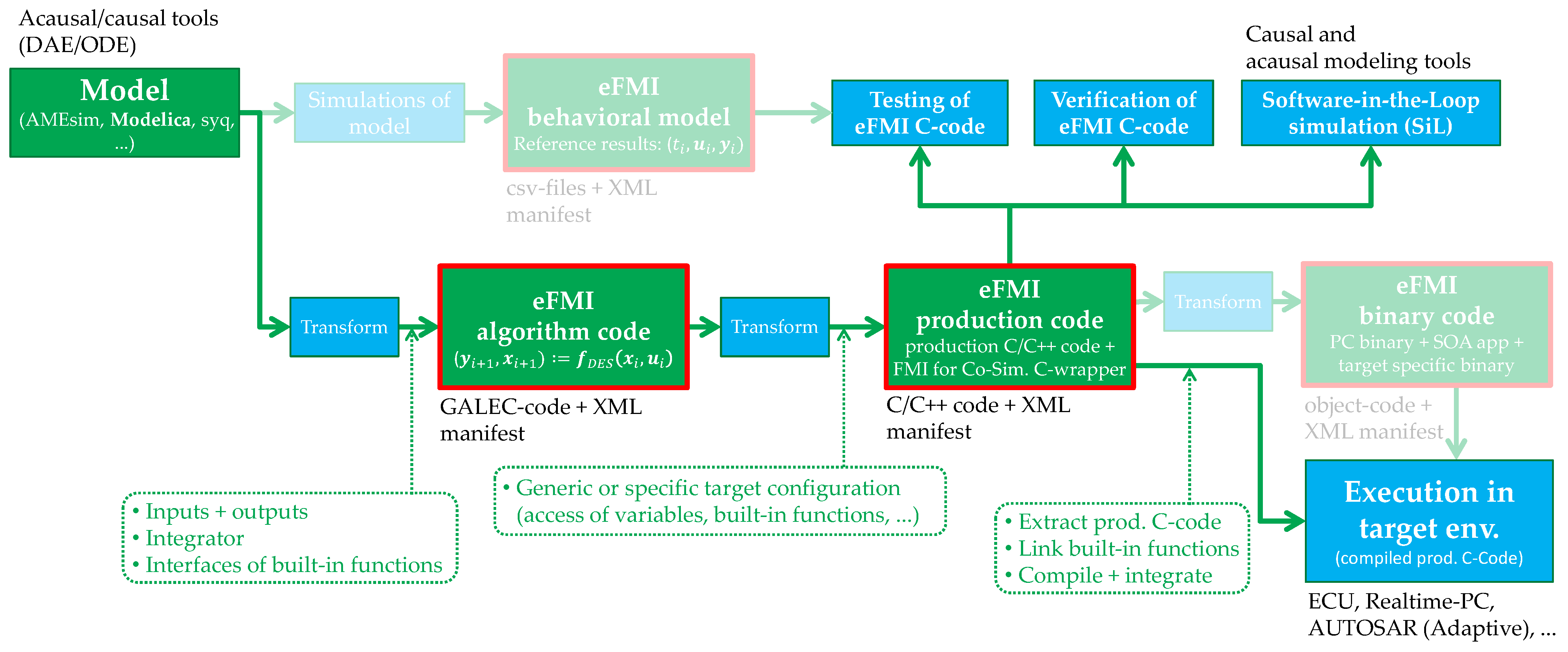
The eFMI Standard provides a workflow which guides and supports the automated deployment of models (e.g., multi-physical models, controllers, estimators) from acausal or causal simulation tools to embedded targets [
10,
11]. The workflow depicted in
Figure 2 consists of various so-called model representations that are stored in containers within a single eFMU. They are derived from the original simulation models via stepwise transformation. The eFMI workflow is summarized in the following. For a detailed description of the workflow and further information on the transformation steps, the reader is referred to [
10].
The simulation environment creates an algorithm code model representation which contains the so-called GALEC (Guarded Algorithmic Language for Embedded Control) code. The GALEC programming language is part of the eFMI Standard and serves as “an intermediate representation between the (physics) modeling and embedded programming domain” [
10] (p. 62). The execution of the algorithm described by the GALEC code on an embedded target requires suitable production code (usually C or C++ code). Regarding the eFMI workflow, this is done by transforming the algorithm code into a production code model representation. After this, the eFMI production code is either directly integrated into the software framework of the embedded target, or a dedicated binary code model representation is generated. Optionally, a behavioral model representation can be generated by the simulation environment. This model representation stores reference results from different simulation scenarios, which can be used to test and verify the production code model representation. Additionally, the eFMI production code can be reintegrated into causal or acausal modeling tools to create a software-in-the-loop (SiL) simulation. This setup may be used for testing or parametrizing the production code in combination with a high-fidelity plant model.
The use-case presented in this paper follows the highlighted path of the eFMI workflow overview in
Figure 2. Modeling and simulation were conducted in Dymola, a modeling and simulation environment for Modelica. Here, an early Dymola prototype with the ability to export the eFMI algorithm code model representation from Modelica models was used. The transformation to the eFMI production code model representation was performed by a prototype of dSPACE TargetLink.
4. The Controller Design Process Using the eFMI Workflow
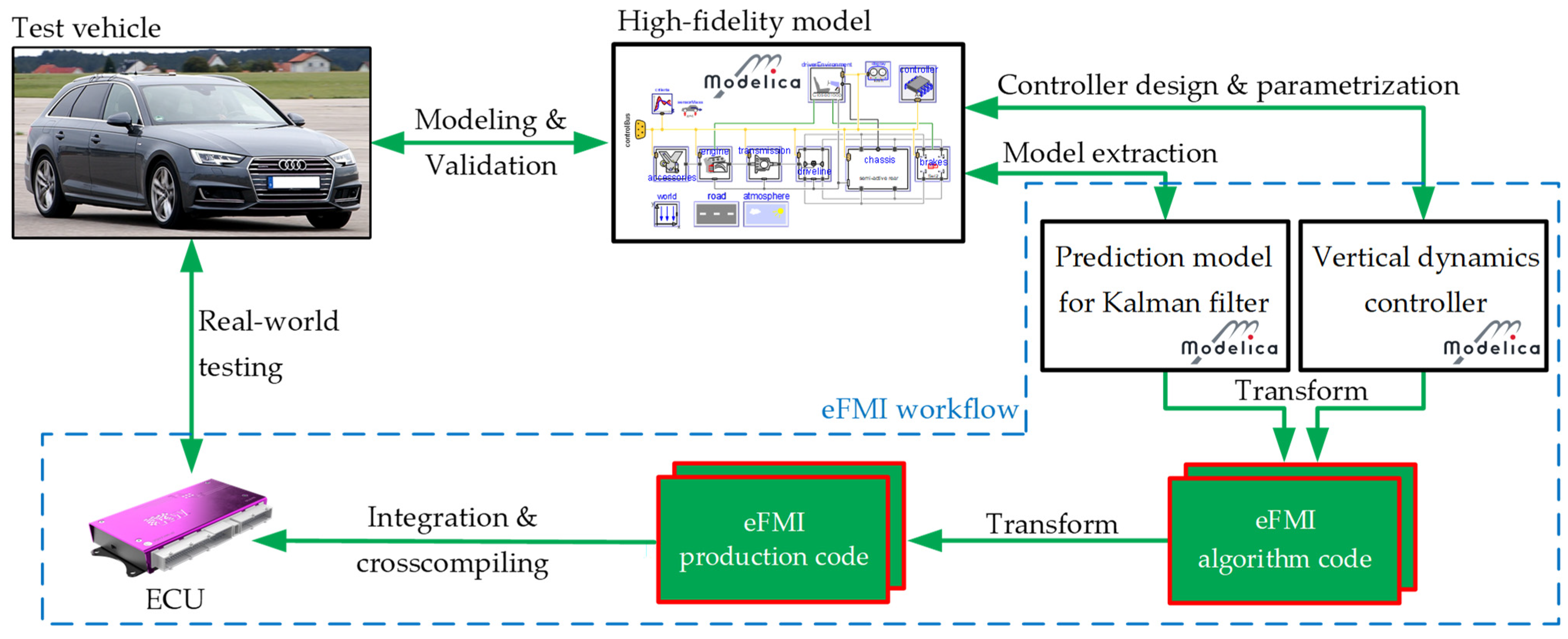
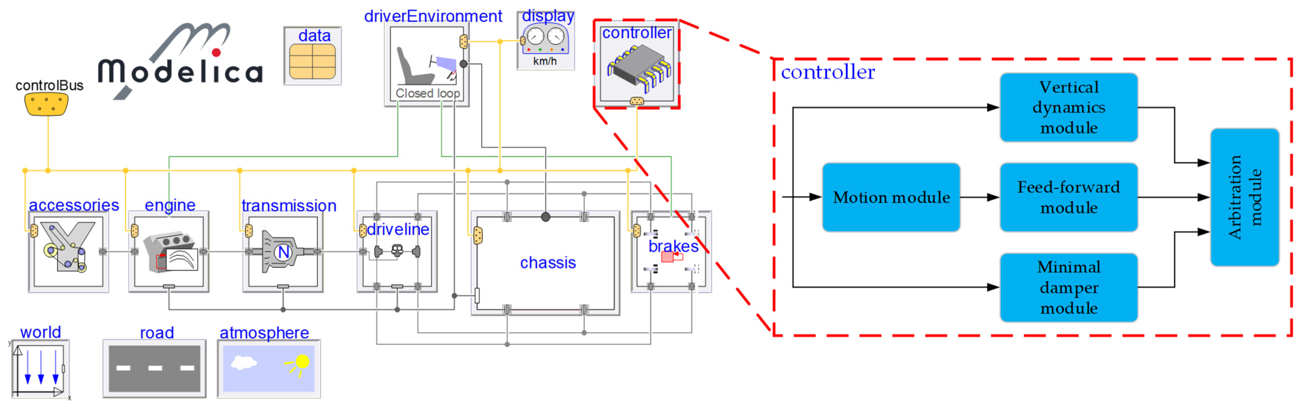
The entire development process of the vertical dynamic controller and the prediction model for the nonlinear Kalman filter is depicted in
Figure 3. The eFMI workflow was utilized in the steps bordered with a blue dashed outline. The overview shows that this workflow closes the gap between the acausal modeling language Modelica and the deployment of the controller on an ECU. The stacked green boxes illustrate the usage of 2 eFMUs: 1 containing the vertical dynamics controller and 1 containing the prediction model for the Kalman filter.
Section 4.1 starts with the first step of the design process, the modeling of the high-fidelity model and its validation. After that,
Section 4.2 presents the design and parametrization of the controller and
Section 4.3 showcases the model extraction of the prediction model for the Kalman filter. Subsequently,
Section 4.4 and
Section 4.5 explain the generation of the eFMI algorithm code and production code model representations. Finally, the integration of the generated eFMUs into the ECU software framework is described in
Section 4.6.
4.1. Assembling the High-Fidelity Model
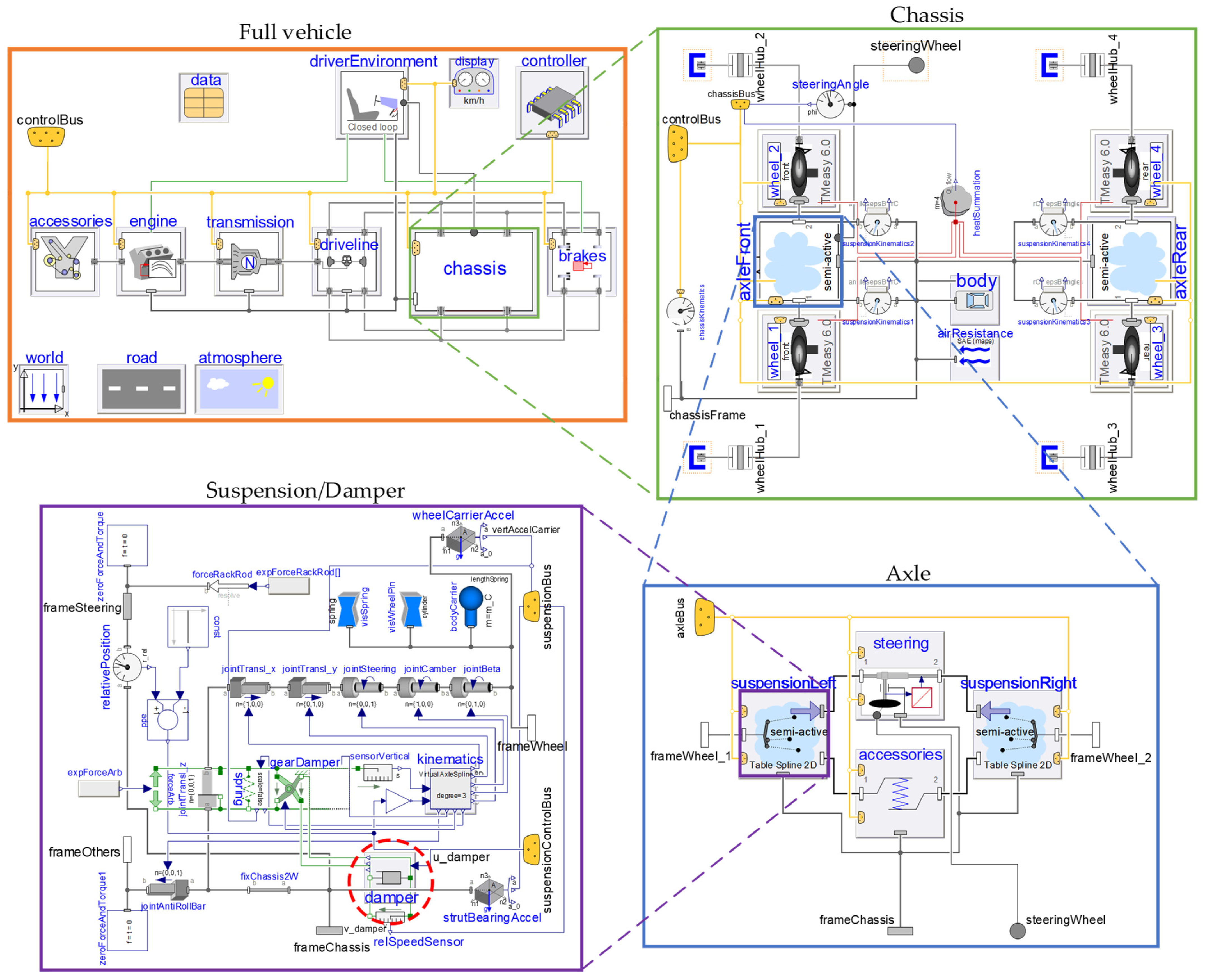
In the early design stage, the controller was tested and parametrized in a closed-loop offline simulation utilizing a high-fidelity vehicle model. This vehicle model comprises several physical domains such as multi-body mechanics of the chassis or a thermal brake model, all implemented using the Modelica language as follows in detail.
On the top level of the model, a full vehicle architecture is given, including the vehicle chassis, power train, and controller (described in
Section 4.2), as well as the driver and the vehicle environment (see
Figure 4). These single modules comprise hierarchical submodels, as demonstrated by the example of the chassis in
Figure 4. Here, the chassis is completed by 2 axles, 4 wheels, and a rigid body. An axle submodule contains the left and the right suspension and optional structures such as a steering assembly and an anti-roll bar. Finally, the suspension reflects a particular mechanical structure, including the semi-active damper.
To calculate the tire/road contact forces, an interface to the semi-physical tire model TMeasy 6.0 [
15] was implemented in Modelica [
16]. TMeasy combines the normalized longitudinal, lateral and turn slips into a 3-dimensional slip, and thus enables a smooth transition from normal driving situations to standstill and vice versa. It provides first-order transient tire dynamics by default and can optionally include higher-order dynamics for given parameters.
The easy interoperability of the internal Modelica automotive libraries is guaranteed by the consistent interfaces defined in the Modelica VehicleInterfaces library [
17]. This library standardizes the interface definitions and enables modularization of vehicle model architectures. It also utilizes a feature of Modelica—an expandable connector called controlBus. Using this connector, the signals can be consistently propagated through the model hierarchy. In particular, the input signal for the semi-active damper is prescribed in the top-level controller.
Due to its dominant influence on the vertical dynamics, particular attention was given to the spring/damper modeling. In this work a specially developed semi-active damper with one external controllable electromagnetic valve was used. The adjustment of the damper force is realized by controlling the electric current flowing through the inductor of the electromagnetic valve. The induced magnetic field imposes the position of the valve piston, and consequently the oil flow through the valve depending on the actual shaft velocity.
An empirical model based on a 2-dimensional force map as a function of the damper velocity and the electric current was chosen to reproduce the highly nonlinear behavior of the semi-active damper. The valve dynamics are approximated through a first order transfer function with an additional time delay. Due to the anisotropic characteristics, the parametrization changes with the movement direction of the damper. The damper model does not include the physical hydraulics equations but still gives reasonable results with acceptable computational effort.
The full-vehicle Modelica model has about 130 states and yields a system of 27 nonlinear equations. It was parameterized for the utilized test vehicle (Audi A4, production year 2016) and cross-checked against a reference table-based vehicle dynamics model provided in another simulation tool, which is widely established in the automotive industry. The validation was performed by means of representative driving maneuvers. Various tests were performed to validate the vertical dynamics (e.g., driving over an obstacle) as well as the lateral and longitudinal dynamics (e.g., steady-state circular tests and coasting or straight-line braking). The simulation results matched well with the reference values, thus proving the validity and accuracy of the Modelica model. To enable fast repeated simulations of different scenarios for the controller parametrization, a fixed step solver was used.
4.2. Design and Parametrization of the Controller
The controller used for the deployment on the ECU is an extended version of an already existing vertical dynamics controller described in [
13]. As depicted in
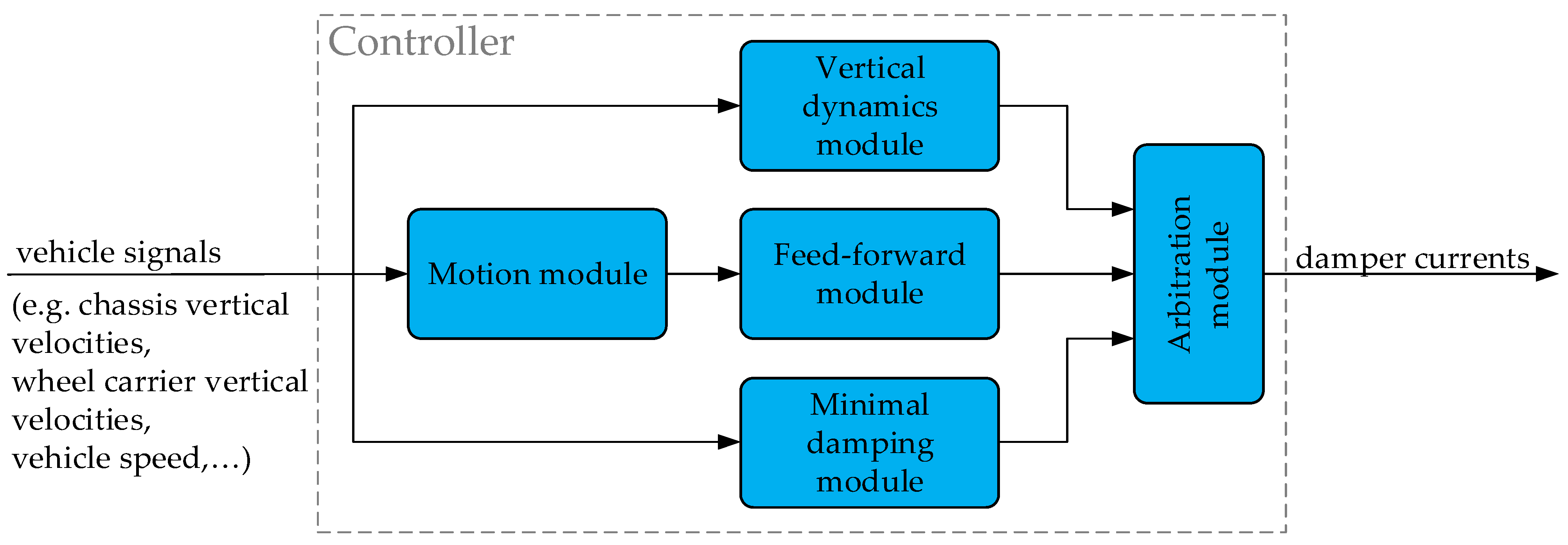
Figure 5, the controller is assembled out of several modules which are designed to account for different requirements and different kinds of excitations (see
Section 2).
The controller calculates 4 damper current setpoints which are inputs to a subordinated current controller. To calculate the current, the controller requires different vehicle signals as input: For each suspension unit the wheel carrier vertical velocity, the chassis vertical velocity near the damper mounting point, and the damper velocity are needed. Additionally, common vehicle signals like vehicle longitudinal velocity, actual gear, accelerator and brake pedal position, steering wheel angle, etc., were utilized within the controller. The different modules presented in
Figure 5 were designed for the following purposes:
Vertical dynamics module: This module is designed to account for road-induced disturbances. A skyhook controller addresses the comfort requirement by controlling the dampers in such a way that the chassis vertical acceleration is minimized. In addition, this module also includes a groundhook controller which minimizes the dynamic wheel load to comply with the road holding requirement.
Motion module: This module predicts the vehicle motion resulting from the driver inputs. For example, the vehicle stationary lateral acceleration is calculated from the steering wheel angle by means of a steady-state single-track model. The vehicle longitudinal acceleration is determined from the accelerator or brake pedal inputs and additional signals (e.g., gear or vehicle velocity).
Feed-forward module: The aim of the feed-forward module is to compensate the driver-induced disturbances based on the predicted vehicle motion. Based on the predicted longitudinal and lateral acceleration at the vehicle’s center of gravity, geometric relationships are used to calculate the damper forces required to compensate for the resulting chassis pitch and roll motion. By means of an inverse damper model, the required force is mapped to a damper current. However, only dissipative forces within a fixed operating range can be applied, since semi-active dampers are used.
Minimal damping module: This module additionally ensures driving safety and overall vehicle stability by limiting the minimum damper force. For this purpose, a characteristic curve is used that depends on the vehicle velocity and increases the damping with rising vehicle velocity.
Arbitration module: Inside this module, the electric current outputs of the abovementioned modules are collected and blended, and 4 damper current setpoints are calculated. The blending is done independently for each wheel, since the vertical dynamics, feed-forward, and minimal damping modules each calculate 4 damper currents (1 for each wheel).
More than 20 controller parameters of the different submodules have to be determined for the experimental tests of the vertical dynamics controller on the hardware of the real vehicle. For this purpose, the Modelica model of the controller is, as depicted in
Figure 6, integrated into the high-fidelity vehicle model presented in
Section 4.1. Different driving maneuvers, both with road- and driver-induced vertical dynamic excitations, are simulated to tune the controller parameters by evaluating suitable objective functions. In general, an objective function may consist of multiple subfunctions, resulting in a multi-criteria optimization problem. For the vertical dynamics control problem, body accelerations (comfort) as well as the dynamic wheel load (road holding) are the key optimization criteria, as discussed in
Section 2. To minimize these key criteria, numerical optimization can be applied to tune the controller parameters (controller gains, thresholds, allocation ratios, …).
4.3. Design and Parametrization of the Prediction Model
In cases where direct measurement of the required control system variables is impossible for technical or economic reasons, Kalman filters can be used to estimate these variables. To obtain a state estimation through a Kalman filter algorithm, a mathematical prediction model of the plant is necessary.
The vertical dynamics controller described in
Section 4.2 relies on the vertical velocities of the wheel carrier, vertical velocities of the body as well as damper deflection velocities and damper/spring deflections. A convenient way to obtain these signals is the use of acceleration sensors and level sensors. One possibility for reconstructing the desired signals from these acceleration and position measurements is the use of a nonlinear Kalman filter.
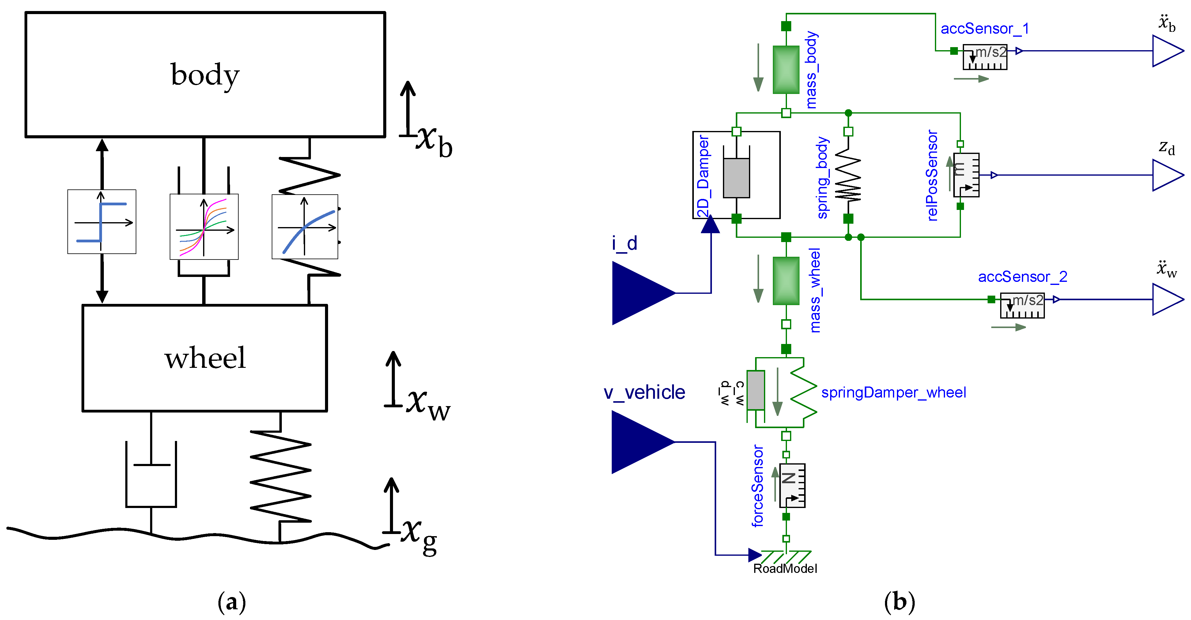
The prediction model for the state estimation is implemented in Modelica and is based on the work presented in [
18]. Considering accuracy and the real-time requirement on the embedded target, a nonlinear quarter vehicle model is chosen as a trade-off. It incorporates a 2-mass system as a simplification of the multi-body dynamics. The masses of all suspension components are proportionally distributed between the quarter vehicle body mass and the wheel mass. The 2 masses are linked by a nonlinear spring-damper unit. The damper was modeled by means of a current-speed-force map. A 2-dimensional linear interpolation was used to obtain the values in between the grid points. The state vector
of this model is given by:
This vector includes the position
and the velocity
of the body and the position
and the velocity
of the wheel, as well as the position
of the ground.
Figure 7a shows the nonlinear 2-mass system with the body and wheel as well as the respective positions. More details regarding the incorporated physical model can be found in [
18].
Figure 7b shows the corresponding Modelica implementation of the nonlinear 2-mass system. The inputs of the prediction model are the velocity of the vehicle and the damper current, while the model returns the acceleration of the body, the acceleration of the wheel, and the damper deflection
. The state equations are described in [
18]. The nonlinear parts of the 2-mass system are contained in the state equations. They include the damper characteristics and the transformation ratio linking the body and wheel motion with the spring-damper deflection, as well as the overall friction force
. This friction force comprises the friction of the joints of the suspension system and the friction of the damper. The formulas for computing the damper force
and the friction force
are given by:
with the transformation ratio
, the current-speed-force map
, and the constant sliding friction
. The tanh function specifies the direction of the friction force. It represents a smooth approximation of the sign function to remove the discontinuity during a change in direction, which is numerically challenging. The parameter
determines the transitional characteristics of the tanh function.
The parameterization was adapted to be performed on the Audi A4 test vehicle. Further details on the Kalman filter such as the used measurements and the filter design process are presented in
Section 4.6.1.
4.4. Generation of eFMI Algorithm Code Model Representations
An important step in the eFMI workflow (see
Figure 2) is the generation of the algorithm code model representation. In our application, the presented multi-physical Modelica models are transformed to real-time algorithms in GALEC. The GALEC code contains a well-defined block interface with inputs, tunable parameters, and outputs (see [
10,
11]). Three block methods are provided:
Startup for initialization of all internal and interface variables,
Recalibrate for the computation of dependent parameters when values of tunable parameters are changed and
DoStep for the computation of the block outputs at each sample time depending on the inputs and internal state variables.
The internal state variables are globally defined inside the block but are not exposed to the outside through the block interface. Within the listed block methods, special built-in functions can be called. These functions are standardized in the eFMI Standard to evaluate common mathematical functions, e.g., sin or exp, but also higher-level functions to solve linear systems of equations or to interpolate data points in 1, 2, or 3 dimensions.
In a Modelica tool (e.g., Dymola), the transformation from a Modelica model to GALEC code covers several steps. A fundamental step is the model discretization in time. Thus, a real-time capable numerical integration method must be applied to the system of differential equations in the model. Because the Modelica language supports a variety of language constructs, these may lead to nonlinear and mixed integer/real systems of equations. Solving these in real-time on an embedded target poses a major challenge. From a practical point of view, the most important Modelica features required in applications need to be supported by the used Modelica tool when exporting the model to an eFMI algorithm code model representation.
The nonlinear controller model in Modelica, described in
Section 4.2, contains a nonlinear inverse model in the feed-forward part, signal filters, and 1- and 2-dimensional interpolation tables, as well as
reinit/
when statements in Modelica language. All these features are supported in the considered eFMI toolchain by the involved prototypical tools. This manifold of different model properties represents a set of typical requirements for model-based controller design in industrial applications. Thus, the controller presents an appropriate set of features to test the applicability of the novel eFMI Standard, the eFMI workflow, and the eFMI supporting tool prototypes.
4.4.1. Algorithm Code of the Controller Model
The controller model in Modelica (see
Section 4.2) is exported to an eFMI algorithm code model representation by a Dymola prototype. The Modelica model containing the continuous model equations of the controller is automatically discretized by Dymola using an Explicit Euler method with a step size of 1 ms. The resulting eFMU contains the GALEC code of the controller.
To illustrate the eFMU export, the filter model Modelica.Blocks.Continuous.CriticalDamping from the Modelica Standard Library [
19] is considered. Instances of this filter model are contained in the controller model. The Modelica code of the filter reads as follows:
| block CriticalDamping |
| … |
| equation |
| | der(x[1]) = (u − x[1]) * w; |
| … |
| end CriticalDamping; |
It defines the differential equation
for the continuous state
, with the filter input
and a fixed parameter
. In the exported eFMU of the controller model, this differential equation is transformed to algorithmic statements according to the selected discretization method. In this exemplary case the Explicit Euler method is used. Regarding the complete controller model, the following GALEC code of the eFMI DoStep method is generated:
| method DoStep |
| … |
| algorithm |
| … |
| | self.‘vertDyn.criticalDamping[2].x[1]’: = |
| | | (self.‘vertDyn.criticalDamping[2].x[1]’ + |
| | | | (self.‘discrete.stepSize’ * |
| | | | self.‘derivative(vertDyn.criticalDamping[2].x[1])’)); |
| … |
| | self.‘derivative(vertDyn.criticalDamping[2].x[1])’: = |
| | | ((self.‘vertDyn.multiplex2.u1[2]’ – |
| | | | self.‘vertDyn.criticalDamping[2].x[1]’) * |
| | | | self.‘vertDyn.criticalDamping[2].w’); |
| … |
| end DoStep; |
The global variables of the eFMI block have the prefix self. In the first statement, the Explicit Euler step is performed for the state . The constant step size is stored in the variable self.‘discrete.stepSize’. The Explicit Euler method requires the computation of the state derivative after the state update. The derivative variable is initialized in the call of the eFMI Startup method before the first call of DoStep.
4.4.2. Algorithm Code of the Prediction Model
The Dymola prototype is also used to export the prediction model (see
Section 4.3) to an eFMI Algorithm Code model representation. The discretization method (Explicit Euler) and the sample time of 1 ms are identical to the ones for the controller model (see
Section 4.4.1). For the current-speed-force map in the prediction model, it is important that the eFMI built-in function for 2-dimensional interpolation is supported by the involved tools.
Assuming the following system of ordinary differential equations
with continuous states
, inputs
, and outputs
for the continuous model part of the Modelica model, the following dependencies remain after the discretization in the DoStep method for each sample time
:
In the standard case the GALEC code of DoStep is optimized to call this method only once at each sample time. For this purpose, the vector may contain more variables than the components of the continuous states (e.g., derivatives of the states or inputs from the previous step).
The prediction model for a nonlinear state estimation requires special features for correct execution within the state estimation algorithm. One important feature is the ability to set discretized continuous states before each call of the DoStep method. This functionality is crucial for certain Kalman filter algorithms that perform multiple integration steps from perturbated states (see e.g., [
20]). For certain nonlinear Kalman filter algorithms, e.g., for the extended Kalman filter method, the computation of the state derivatives
is needed.
There is no prototypical implementation of an eFMI exporter with the desired functionality available. In this work the necessary features are manually coded based on the standard GALEC code generated by Dymola. The code is manually prepared to eliminate assumptions about the order and number of calls of the DoStep method that are introduced for the standard call at 1 sample time. Further, the evaluation of each of the following three categories of variables is separated and can be called individually:
The function in Equation (6) computes the state update via an integration method. Its interface is generic for many integration methods, especially for typical one-step methods, like the Explicit Euler method, which is usually applied in real-time simulation.
4.5. Generation of eFMI Production Code Model Representations
The next step according to the eFMI workflow is to transform the algorithm code to production code, as shown in
Figure 2 and
Figure 3. Higher demands are made on production code for embedded systems, especially for safety-critical systems. For instance, there are strict limitations in data and code size. In addition to that, dynamic memory allocation is not available. Standard library functions for embedded targets are hardly available, and proper error handling as well as the fulfillment of coding rules like MISRA C:2012 are required [
10].
The eFMI Standard defines how production code is incorporated in an eFMU by the production code model representation. The tools specialized in production code generation read the algorithm code model representation of an eFMU and add several production code containers to the eFMU, each generated for dedicated software integration scenarios. In contrast to the FMI Standard, there is no defined C code interface for the main functions (DoStep, …) in eFMI. For example, the code variants may differ in floating-point data types (e.g., 32-bit vs. 64-bit), in the data structure of the variables, or in the interface realizations of functions (e.g., global variables vs. function parameters) [
10].
The eFMI production code model representations for both the controller and the prediction model are generated by a TargetLink prototype via processing the algorithm code model representations described in
Section 4.4. For both eFMUs the C code generation in TargetLink is configured to support the integration of the controller C code and the prediction model C code into 1 C software project without manual adaptions of the C code like renaming of variables or types. The model representations generated with 64-bit floating-point support are used in software-in-the-loop tests, whereas the 32-bit variants are dedicated for integration into the embedded system.
The production code of the prediction model is manually adapted to enable write access to the discretized continuous states before each call of the DoStep function. This is required for the application of an eFMU in a nonlinear Kalman filter algorithm and is currently not covered by the published eFMI standard 1.0.0 alpha 4 [
11].
4.6. Integration of eFMUs and Deployment on the ECU
For the execution on an embedded target, it is necessary to further process the generated eFMUs with production code. This concerns both generated eFMUs (the controller eFMU as well as the eFMU for the prediction model, which is incorporated into a nonlinear state estimation environment). Since they are both applied on a low-volume production series ECU, the production code of the eFMUs must be integrated into the basic software framework of the ECU. The steps in this integration process are described in the following subsections.
4.6.1. Integration of the eFMU into the Embedded Kalman Filter C-Library
To accomplish the state estimation, a specialized embedded Kalman filter library [
21] is applied that is based on the internally developed Kalman filter library (for more information see [
20,
22]). All parts of this new library, in contrast to that mentioned previously, are implemented in pure C without external dependencies. It therefore represents a self-contained implementation. Since the library is available in a 32-bit configuration, it is suitable for use on embedded systems. The embedded Kalman filter library contains implementations for the extended Kalman filter with square-rooting (EKF-SR) and the unscented Kalman filter with square-rooting (UKF-SR). Details about these estimators can be found in, e.g., [
23]. For the toolchain described in this paper, the EKF-SR is employed. It has the advantage of reduced complexity, as opposed to the UKF-SR, and thus a shorter execution time is achieved. Therefore, the EKF-SR is well-suited for practical usage in real-time applications with short sample times.
The generated production code representing the prediction model (see
Section 4.5) is integrated into the filter code to calculate the model evaluations. The DoStep function is therefore called several times at each sample time to calculate the evaluations in Equation (6). This function provides the computation of the outputs as well as the derivatives of the states that are required for the EKF-SR. In addition, the states of the model are computed through integration between 2 sample points.
Furthermore, the parameterization of the Kalman filter algorithms represents a challenging issue and can be carried out with the help of various methods, see e.g., [
24]. In this paper, the filter parameters (system and measurement noise covariance matrices) are determined using a reference trajectory and minimizing the error between the estimated and the true states. The optimization is performed using the optimization software MOPS [
25].
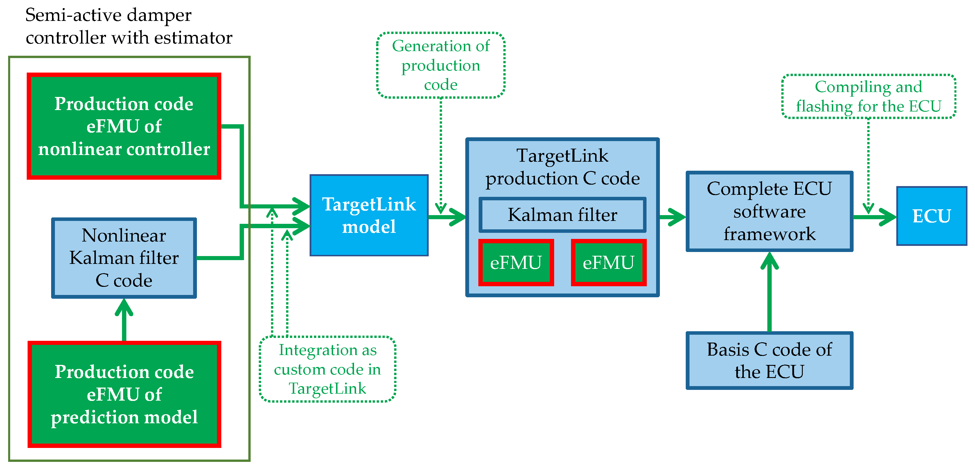
4.6.2. Assembly and Integration of the eFMUs
The state estimator and the semi-active damping controller are both executed on a low-volume production series control unit from our non-funded cooperation partner KW automotive. The main functionalities of the ECU, which are not covered by the control system, are implemented in TargetLink. These functionalities include inter alia fault detection, current controllers, sensor data processing, and mode selection. To utilize the eFMI-based control system, it is necessary to integrate the eFMUs as well as the embedded Kalman filter library into the TargetLink model. This is achieved by using the TargetLink custom code blocks (see
Figure 8).
Using the custom code blocks allows the integration of the eFMU into the code generated by TargetLink without altering the eFMU production code or the embedded Kalman filter library code. Additionally, this enables flawless interaction and signal flow between the eFMUs and different TargetLink modules. Moreover, this workflow reduces the need to manually integrate the eFMI production code into the complete software framework of the ECU. For the final deployment on the ECU, the TargetLink production C code containing the eFMUs is merged with additional basis C code of the ECU and compiled for the target. The basis C code handles low-level functionalities and is provided by the ECU supplier. The entire integration process is depicted in
Figure 8.
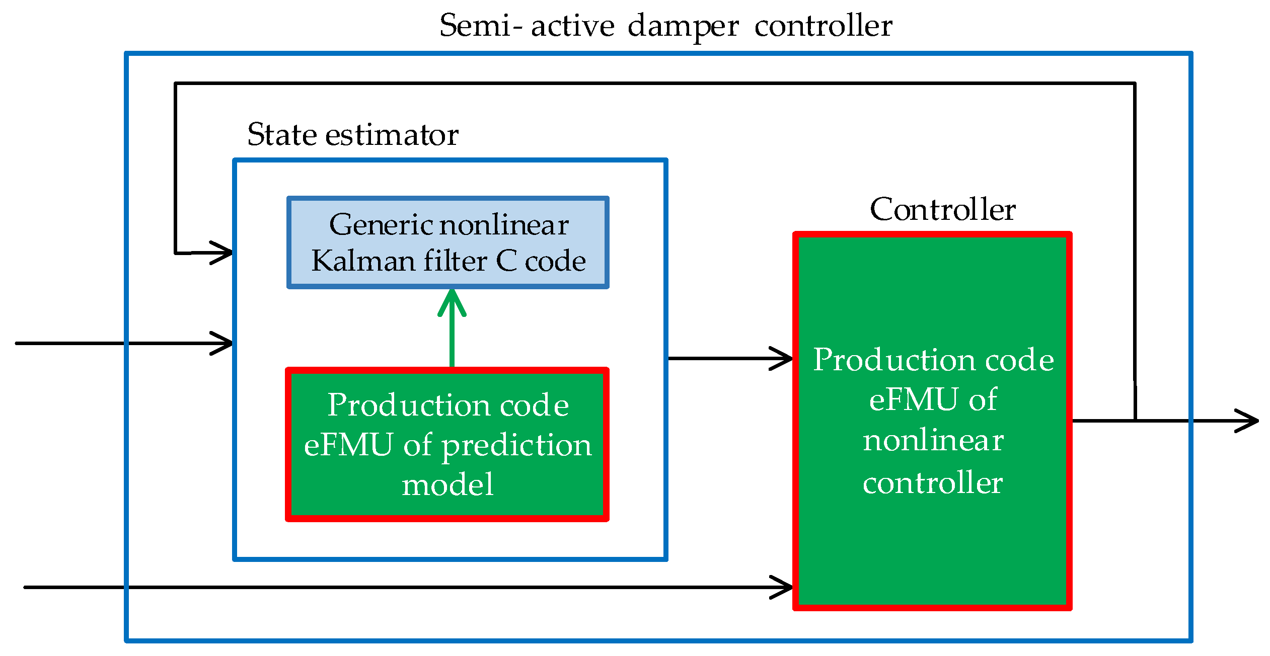
As inputs, the state estimator custom code requires the velocity of the vehicle and the damper currents as well as the measured outputs of the prediction model, respectively the measured vertical acceleration of the body, the vertical acceleration of the wheel and the damper deflection. The estimated states are used as inputs for the controller. The assembly of the controller eFMU, the prediction model eFMU, and the generic nonlinear Kalman filter C code are depicted in
Figure 9.
The controller uses the estimations of the Kalman filter along with additional measured signals (e.g., vehicle speed or steering wheel angle) as inputs. The state estimator exploits sensor signals as well as the fed-back damper current, which is commanded by the controller, to calculate its estimation.
In addition to the state estimation on the ECU, another approach to calculate the required controller inputs is implemented on a rapid-prototyping platform. This is only possible due to the higher numerical accuracy of the rapid-prototyping platform. The calculations on the rapid-prototyping platform can be used to bypass the state estimator. This enables stand-alone testing of the embedded Kalman filter and the controller (not shown in the figure).
Since the ECU has limited computational power, no multitasking features, and a sample-time of 1 ms, the real-time execution of the embedded Kalman filter is challenging. This caused the restriction that the filter could only be executed for 1 damper at each sampling time. However, for industrial applications the filter calculation for all 4 dampers could be performed sequentially across 4 timesteps.
5. Results of Software and Hardware Tests
After carrying out the control system design process for the vertical dynamics controller and the Kalman filter described in
Section 4, we conducted several tests to validate the toolchain and the methodology. For this validation, offline open-loop tests were executed. These tests are described in
Section 5.1. At that stage of eFMI standard development, the tools supporting the eFMI workflow were still prototypical implementations. Therefore, validation tests were necessary to proof the eFMI concept.
To validate the generated eFMUs in real operation, the target ECU with the embedded control system was integrated into an experimental vehicle and tested on a German rural road, as described in
Section 5.2.
5.1. Offline Open-Loop Tests
To test and validate the transformations described by the eFMI workflow (summarized in
Section 3) and to evaluate the Kalman filter library including the prediction model as an eFMU, several offline open-loop tests were performed. The experiments related to the controller eFMU are summarized in
Section 5.1.1. The combined testing of the nonlinear Kalman filter library and the prediction model eFMU is described in
Section 5.1.2.
5.1.1. Validation of the Controller eFMU
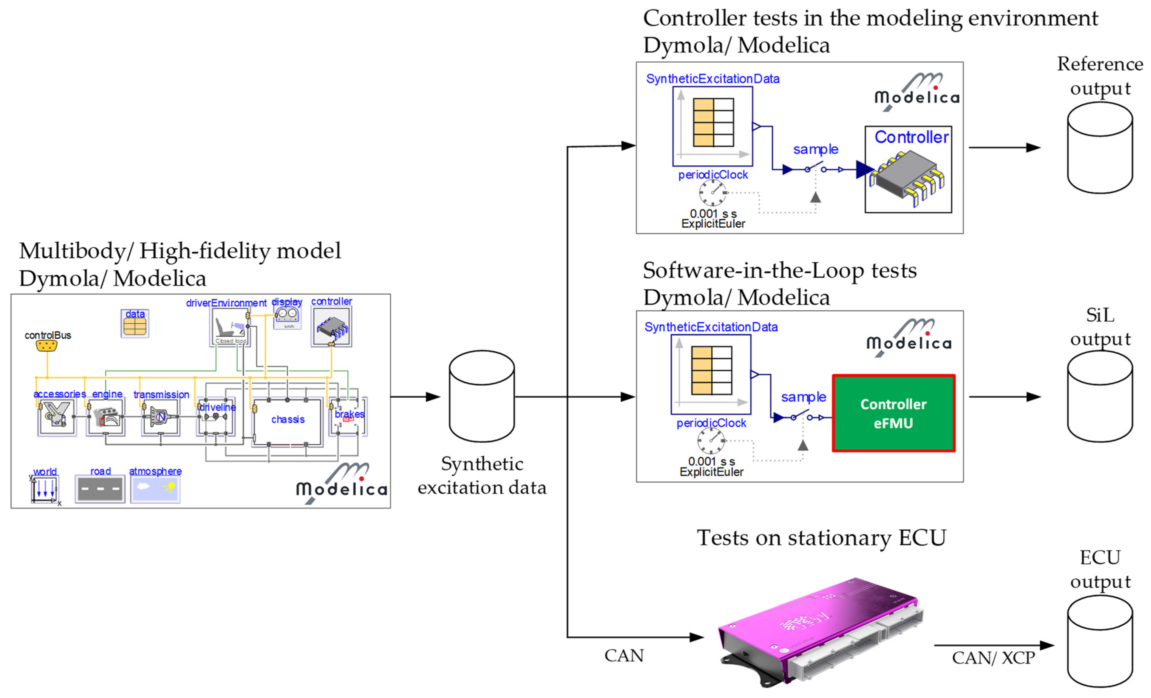
The test setup for validating the eFMI toolchain is depicted in
Figure 10. To stimulate the controller with realistic input data, the high-fidelity vehicle model was simulated with a dedicated road and driver excitation profile. During this simulation, the electric current input of the semi-active dampers was chosen to be constant. The controller input signals were recorded as realistic synthetic excitation data for the subsequent tests.
To obtain reference controller output data (reference output in
Figure 10, above right), the Modelica version of the controller, as described in
Section 4.2, was stimulated with the synthetic excitation data.
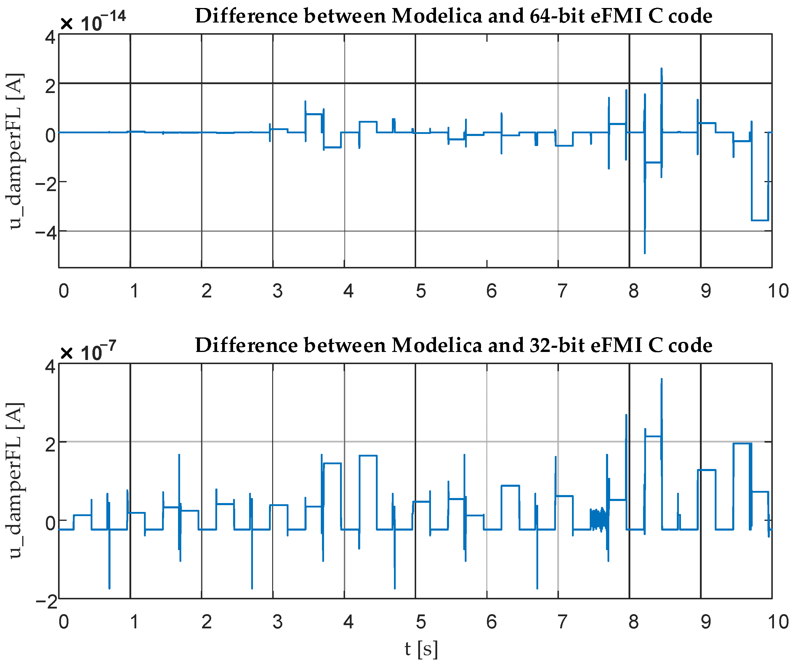
Then, to validate the eFMI transformation steps from Modelica to the eFMI algorithm and production code (cf.
Section 3), the production code was reimported into Dymola and excited with the same synthetic data. Afterwards, both results of the 64-bit variant of the C code and of the 32-bit variant (SiL output) were compared to the reference output of the controller. All these tests showed very good compliance between the Modelica version of the controller and the eFMI production code results in their expected accuracy range (maximum errors less than
for 64-bit and
for 32-bit floating-point precision). Exemplary results are depicted in
Figure 11.
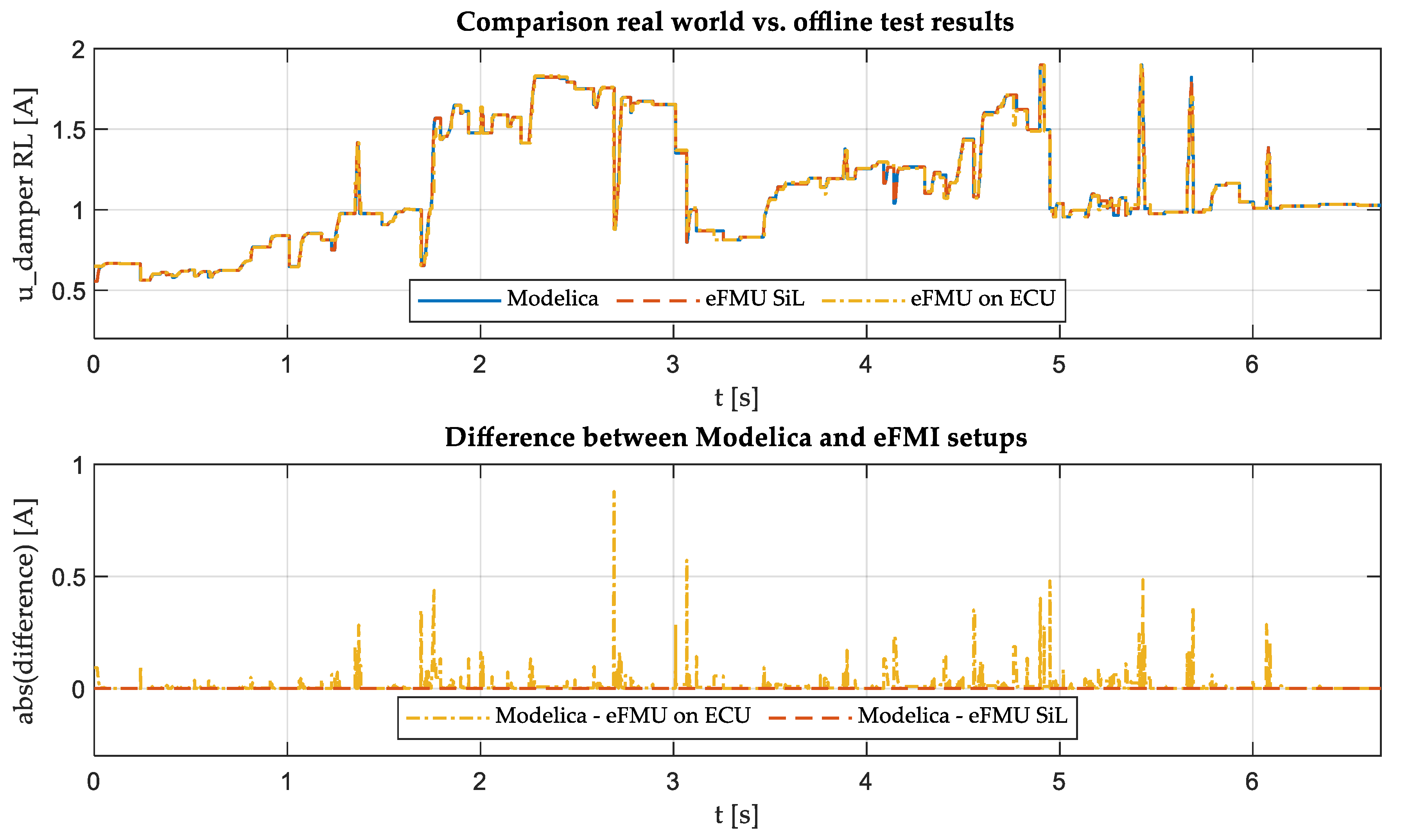
To finally ensure the correct execution on the target ECU, the synthetic excitation data were sent to the ECU via CAN and the outputs of the controller were logged via XCP over CAN (ECU output in
Figure 10, below right). An excerpt of the results from the open-loop tests is provided in
Figure 12.
Overall, the results from the simulations align very well. The observed deviations presumably originate from the fact that sending the signals over CAN to the ECU as well as logging the signals of the ECU via CAN introduces additional delays. This complicates the synchronization of data from the test on the stationary ECU with the SiL tests. The spikes in the difference plot in
Figure 12 are likely caused by jitter in the transmission over CAN/XCP and synchronization inaccuracies. For the steps in the controller output, these small time deviations result in large deviations between the offline open-loop tests results.
5.1.2. Validation of the Kalman Filter Including the Prediction Model eFMU
To validate the performance of the embedded Kalman filter library in combination with the eFMI production code of the prediction model, offline simulations in TargetLink were conducted. As described in
Section 4.6.1 and
Section 4.6.2, the production code representing the prediction model is integrated into the embedded Kalman filter library to perform the model evaluations for the state estimation. To test the estimator, the resulting Kalman filter algorithm (embedded Kalman filter library and prediction model eFMU) is integrated in TargetLink as custom code and simulated.
In this test setup, the inputs for the state estimation custom code were obtained from a recorded simulation of the high-fidelity vehicle model, as in the approach applied and described in
Section 5.1.1. The recorded data contain the inputs for the estimator as well as the reference signals (states of the quarter vehicle model, see
Section 4.3) which are estimated by the Kalman filter.
Figure 13 shows the comparison between the reference states obtained from the simulation of the high-fidelity model and the states estimated by the Kalman filter.
The simulations were carried out with the 32-bit variant of the EKF-SR. Two estimated states of interest from Equation (1) are depicted: the vertical velocity of the body and the vertical velocity of the wheel . The comparison shows that the estimator can follow the dynamics. Nevertheless, deviations between the reference and the estimation may be due to different reasons: The prediction model used in the filter represents only a simplification of the high-fidelity model, which was used to obtain the reference values. On top of that, to emulate the limited calculation precision on the embedded target, the simulation was carried out in the 32-bit version. Additionally, simplified numerical routines were applied to meet the challenging real-time requirements on the ECU.
5.2. Real World Tests
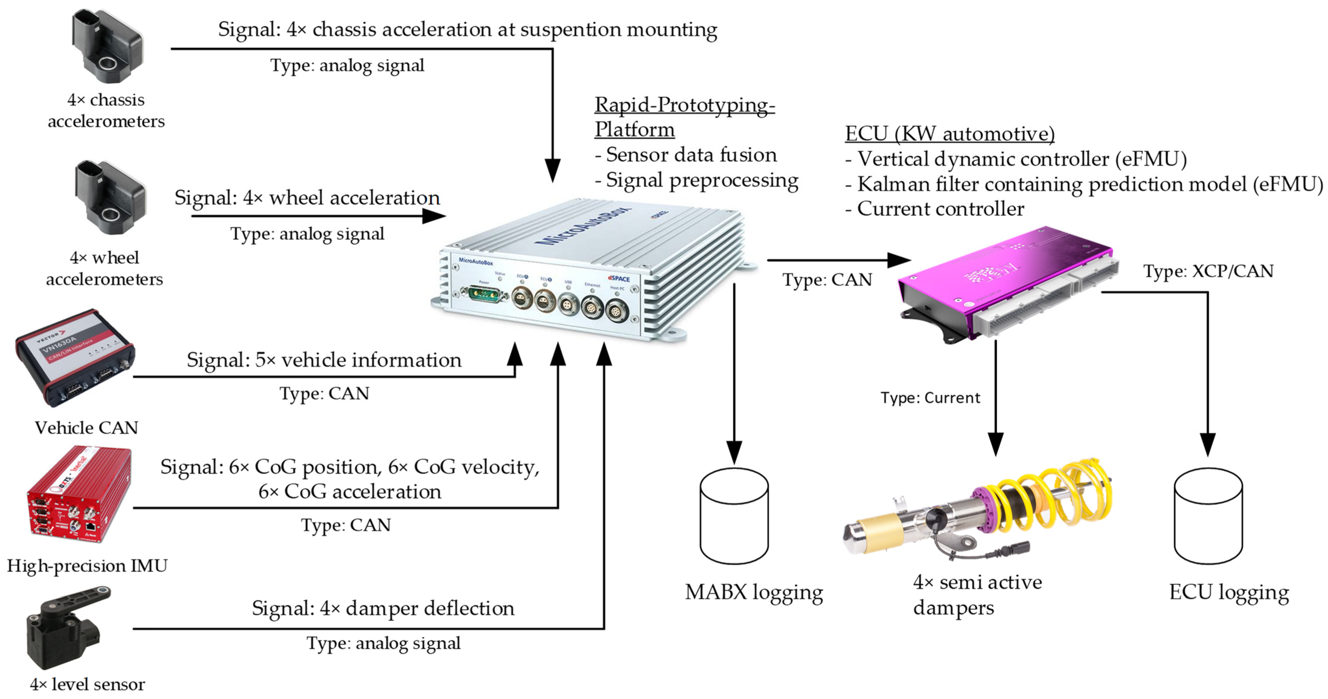
To validate the controller together with the nonlinear Kalman filter in real operation, an Audi A4 test vehicle was equipped with additional sensors as well as a rapid-prototyping platform (dSPACE MicroAutoBox II (MABX)), as shown in
Figure 14. The target ECU is included in the setup as depicted in
Figure 14. In the demonstrator the MABX II performs two main tasks: processing the sensor data and logging the data at a high sample rate of 1 kHz. Because of the bandwidth limitation of the CAN bus, the signals on the ECU can only be logged with a slower sample rate of 100 Hz.
The wheel and chassis accelerations, required by the controller and the estimator, were determined by eight acceleration sensors. They were installed at the suspension mountings on the chassis side and at the wheel carriers on the wheel side. The damper velocity was determined by the numerical differentiation of the damper deflection, which is measured by four rotational potentiometers on each wheel carrier. The vehicle’s internal variables, such as the brake pedal position, were obtained via the vehicle CAN. A high-precision inertial measurement unit (IMU) OxTS RT4000 merged with GPS was used as a reference sensor for analyzing the performance of the controller and the estimator. The test vehicle was also equipped with a 4G/LTE communication module, which enables remote access to all systems in the vehicle.
For the validation of the Kalman filter, the estimates made on the ECU were compared with reference measurements. To obtain the reference variables (body velocity
and wheel carrier velocity
) the corresponding measured variables of the accelerometers were high-pass filtered and then numerically integrated on the MABX. A comparison of these two states for a maneuver on a road rich in stochastic excitations is shown in
Figure 15.
Depending on the maneuver, the filter exhibited different tracking performance. One reason for the varying accuracy is the fact that the filter parameters were optimized exclusively based on synthetic data from the high-fidelity model, and not on the real sensor data with their specific noise characteristics. Additionally, the limited numerical accuracy in the ECU due to 32-bit bit floating-point precision and simplified numeric routines due to the challenging sample time of 1 ms might have reduced the accuracy of the filter. Furthermore, the quarter vehicle model incorporated as prediction model (see
Section 4.3) is the result of simplification and is, like every model, subject to model mismatches. For example, the kinematics of the entire suspension was approximated, and the effects of the bushings were neglected. This may have further affected the quality of the estimation.
To evaluate the respective submodules of the controller separately, different maneuvers were performed. On the one hand, we conducted maneuvers which induced driver-side excitations, such as accelerating, braking, or steering and double lane changes on flat ground. On the other hand, maneuvers with additional road-side excitations (driving over speed bumps with constant velocity) were carried out. Driving on a rural German road yielded a combined excitation. To evaluate the controller performance decoupled from potential inaccuracies caused by the Kalman filter, reference signals calculated on the MABX were used as inputs.
To validate the operation of the controller on the ECU after the real-world tests, the logged sensor data as well as the controller output were synchronized and imported to Dymola. Like the open-loop tests discussed in
Section 5.1, the recorded MABX output data were used to excite the Modelica model as well as the eFMI production code of the controller. The results were then compared to the logged ECU controller output data. An exemplary plot of the results is shown for the rear left damper current in
Figure 16.
As the offline open-loop tests presented in
Figure 11 show, the difference between the Modelica and the 32-bit eFMI SiL version of the controller was in the expected range of
. Therefore, this difference appears to be zero in
Figure 16. In addition,
Figure 16 shows that the logged data during the real-world test “eFMU on ECU” aligned well with the Modelica version of the controller and the 32-bit eFMI production code integrated into Dymola. Besides minor differences, greater deviations between the logged and simulated data could only be observed in rare situations. The mismatches may be related with different effects.
First, as
Figure 14 shows, the excitation data were logged on the MABX. In the test vehicle the sensor data were sent to the ECU via CAN. This signal transmission over CAN causes an additional delay. Another source of error is the fact that the output of the ECU via the XCP on CAN protocol (cf.
Figure 14) could only be logged with a sampling rate of 100 Hz because of the overhead of the XCP protocol. This fact complicated the synchronization of the ECU data logging with the recordings on the MABX. Since the controller has nonlinear characteristics, small deviations in the inputs can result in greater deviations in the output. Based on these issues, we assume that the rare deviations between the signals were for synchronization and numerical reasons rather than systematic errors.
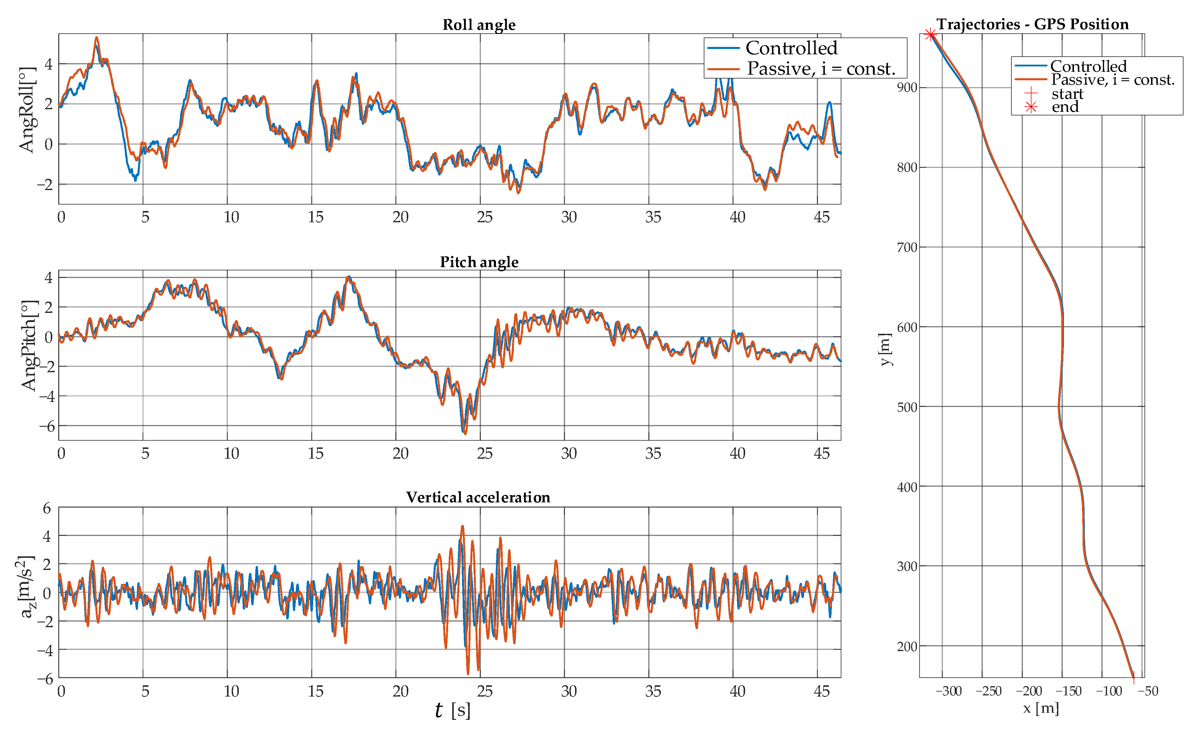
For the validation of the controller in real vehicle operation, comparative maneuvers were performed with an active and inactive controller (passive system). A fixed damper characteristic curve was chosen for the passive system, i.e., the damper currents were set to constant values. To ensure comparability, an identical trajectory had to be driven at the same speed for both setups. For this purpose, a pre-defined path on a German rural road (combined excitation) was driven through with the help of the vehicle’s cruise control system. After the test drive, the GPS position was used to synchronize both positions so that the parameters of interest in terms of vehicle dynamics could be compared.
Figure 17 shows a comparison of the controller with a constant soft damper characteristic curve.
A comparison of the two trajectories showed that an almost identical path was followed in both setups. This allows us to compare the test results of the system in controlled and passive mode.
Figure 17 shows that enabling the controller reduced the oscillations in the vertical acceleration as well as the oscillations in pitch and roll angle. As discussed in
Section 2, reduced vertical chassis accelerations are related to enhanced ride comfort. Since it was not possible to measure the wheel load during the tests on a public road, the effect of the controller on the road holding criterion could not be determined.
In summary, the tests described in this section show that the controller eFMU quantitatively calculates correct results (cf.
Figure 16) and qualitatively influences the vehicle dynamics in the expected manner (cf.
Figure 17). Thus, we demonstrated the entire controller development process supported by the eFMI workflow from multi-physical modeling up to successful real-world testing.
6. Summary and Outlook
In summary, the development, application, and verification of a model-based nonlinear controller in combination with a nonlinear Kalman filter—both based on multi-physical Modelica models—were successfully demonstrated on a low-volume production ECU for semi-active dampers in an experimental vehicle.
The application of the eFMI workflow introduced by the novel eFMI Standard was described in detail. We showed that this workflow closes the gap between the controller development in a high-level modeling language and the deployment on an embedded target. Utilizing the eFMI workflow enables a flawless toolchain for the integration of models and model-based controllers from high-level modeling languages into embedded targets. We showed the successful, stepwise process ranging from modeling, control system design and parametrization, eFMI export and transformation, integration, and deployment up to real-world testing of the control system. We further demonstrated that the transformations between the different eFMI model representation were performed successfully and that the tool prototypes covered a wide range of model properties. Therefore, a multitude of numerical offline tests to validate the transformed eFMU code were carried out. In addition, the necessary modifications to incorporate eFMUs as prediction model for a nonlinear Kalman were described. This enabled the application of Kalman filter methods in combination with the eFMI Standard. Besides the varying performance of the Kalman filter, all results related to the eFMI toolchain showed correct behavior in terms of quality and quantity. The conducted real-world tests of the final controller on an embedded target ECU in an experimental vehicle supported these findings and showed the maturity of the standard and the supporting tools.
Currently, there are missing features in the eFMI Standard and/or the corresponding software tools to directly generate eFMI prediction models for nonlinear state estimators. It is planned to include these requirements in the eFMI Standard and its supporting tools in the future based on the results established in this work.


 ,
, 