Continuous Control Strategy of Planar 3-Linkage Underactuated Manipulator Based on Broad Neural Network

Abstract

For the position control of a planar 3-linkage underactuated manipulator (PTUM) with a passive first linkage, a continuous control strategy is developed in this paper. In particular, a broad neural network (BNN)-based model is first established to accurately describe the motion coupling relationship between the passive linkage and the second linkage. Based on this model, by using the particle swarm optimization algorithm, the target angles of all linkages are calculated combining the start states of all linkages and the target position of the PTUM. Then, the target angles of the active linkages are directly achieved by their respective actuators, and that of the passive linkage is also achieved by the rotation of the second linkage. By carrying out several experiments, the effectiveness of the above strategy is verified.

1. Introduction

An underactuated mechanical system (UMS) is a kind of nonlinear systems with fewer control inputs than the degrees of freedom [1]. The underactuated manipulator (UM) is a typical UMS, which has the features of light weight, low energy consumption and high flexibility [2], so it has the broadly practical application prospects. Moreover, when a fully actuated manipulator (FAM) suffers from the actuator failure, using the control strategy of the UM can ensure the FAM to run normally [3]. Therefore, the growth of the control strategy of the UM indirectly improves the reliability of the FAM. With the growths of the aeronautical engineering and the deep sea exploration engineering, the motion control of the planar UM in the absence of gravity has become one of the hottest topics in the fields of the nonlinear system control and robot control [4].

In an ideal situation, there is no friction at the joints of the planar UM. Hence, the planar n-linkage UM (PNUM) with a passive first linkage (n > 2) has a first order nonholonomic constraint (FONC) [5]. The FONC illustrates that the passive linkage is static when all active linkages are static, which provides a guidance for the stable control of the PNUM [6]. Based on the FONC of the PNUM, some control strategies have been proposed to achieve its position control. Ref. [7] presents a model reduction-based control strategy for the PNUM. The PNUM is reduced to a planar virtual 3-linkage UM with a passive first linkage and two planar virtual 2-linkage Acrobots in turn. Considering that the planar virtual Acrobot has a holonomic constraint which interprets the relationship between the angles of the passive linkage and the active linkage [8], the angle control of the passive linkage of the PNUM can be achieved by dint of the holonomic constraints of two planar virtual Acrobots. Thus, the position control target of the PNUM can then be realized. Nevertheless, the model reduction-based control strategy is implemented with several control stages, which directly leads to the complicated controller design and long control time. To solve these problems, Ref. [9] proposes a continuous control strategy in accordance with the differential evolution algorithm to quickly fulfil the position control target of the PNUM. In this reference, a motion coupling relationship is developed to replace the holonomic constraint of the planar virtual Acrobot to achieve the angle control of the passive linkage of the PNUM.

The above control strategies are presented for the PNUM without considering the joint friction. However, for a real PNUM, the frictions at the joints are objective realities [10]. Thus, the real PNUM with a passive first linkage does not have the FONC, and it is even impossible to fulfil the angle control target of the passive linkage by means of the holonomic constraint of the planar virtual Acrobot. Namely, the control strategies in Refs. [7,9] are only proposed from the theoretical point of view, and cannot be used for the position control of the real PNUM. Therefore, it is vital to develop a feasible position control strategy for the real PNUM.

The greatest difficulty in the position control of the real PNUM is how to fulfil the angle control target of the passive linkage. Because of the lack of the actuator, the angle control of the passive linkage can merely be achieved by controlling the active linkages [11]. Thus, finding the motion coupling relationships (MCRs) between the passive linkage and the active linkages is the crux to fulfil the angle control target of the passive linkage. In general, the MCRs are evolved from the dynamic model of the PNUM [12]. Nevertheless, due to the existences of uncertain factors (such as, the frictions, joint clearances, parameter perturbations and so on) [13,14], it is hard to construct a precise dynamic model expression for the real PNUM. Therefore, it is necessary to explore a more effective method to get the MCRs between the active linkages and the passive linkage.

In recent years, the deep neural network (DNN) has been widely used to depict the complicated nonlinear mapping relationships [15,16]. Comparing with the shallow neural network, the DNN has a higher prediction accuracy [17,18]. However, there are still some problems when using the DNN, such as the complex model structure and the time-consuming training. To solve these problems, some scholars propose a new type of neural networks called broad neural network (BNN) [19,20]. The BNN is an emerging flat network, which shows the outstanding performance in regression problems [21,22]. Moreover, the BNN also has the features of simple network structure, fast training speed and good generalization performance [23], which can effectively overcome the shortcomings of the DNN. Therefore, for a real PNUM, the BNN may provide a feasible way to establish the model that can accurately depict the MCRs between the passive linkage and the active linkages.

On the basis of the above considerations, a continuous control strategy in accordance with the BNN is presented for the planar 3-linkage underactuated manipulator (PTUM) with a passive first linkage to rapidly achieve its position control. Firstly, we establish a model based on the BNN to accurately depict the MCR between the passive linkage and the second linkage. Then, according to the start state of each linkage, the target position of the end-point and the BNN model, the target angle of each linkage of the PTUM is calculated by using the particle swarm optimization (PSO) algorithm. Afterwards, in accordance with the start angle and the target angle of the second linkage, the rotation angle of the second linkage is calculated, and then the passive linkage is controlled to its target angle through one rotation of the second linkage. Due to the weak coupling between the third linkage and the passive linkage, the rotation of the third linkage has few influences on the state of the passive linkage and can be ignored. Therefore, while the second linkage is rotating, the third linkage is controlled to its target angle with low rotating speed. Eventually, the availability of the presented position control method is demonstrated by three sets of experimental tests.

2. Establishment of BNN Model

The control of the passive linkage is the crux to fulfil the position control target of the PTUM. Because of the lack of actuator, the passive linkage can merely be jointly controlled by the MCRs between the passive linkage and the active linkages, which are commonly evolved from the dynamic model of the PTUM. Nevertheless, the accurate dynamics model expression of a real PTUM is hard to be obtained due to the uncertainties (such as, frictions, joint clearances, parameter perturbations and so on). Therefore, in this part, we employ a data-driven modeling method to build a model which can depict the MCRs between the passive linkage and the active linkages, thus preparing for the position control of the PTUM.

The data-driven modeling method is based on a large amount of the input and output data [24]. The corresponding data mapping relationship can be established without understanding the internal mechanism of the object [25]. Currently, lots of data-driven modeling methods have been put forward, such as the multi-layer perception modelling method [26], support vector regression modeling method [27], BNN-based modeling method and wavelet neural network modeling method [28]. Among them, the BNN-based modeling method has the features of simple structure, fast training speed and good generalization performance [29,30]; thus, it is particularly suitable to establish the model that can accurately depict the MCRs between the passive linkage and the active linkages. So, we choose the BNN-based modeling method in the following developments.

Note that there exists couplings between the passive linkage and the second linkage and between the passive linkage and the third linkage. However, the coupling degree of the former is higher than that of the latter because the passive linkage and the second one are direct-coupled. So, only using the MCR between the passive linkage and the second one can realize the control target of the passive linkage. Based on that, next, we only need to employ the BNN-based modeling method to construct the MCR between the passive linkage and the second linkage.

Through a lot of experimental tests, we discover that the rotating angle of the passive linkage $\Delta q_1$ is determined by the rotating angle and angular velocity of the second linkage ${\dot{q}}_2$ and $\Delta q_2$, and the start angle of the passive linkage $q_{10}$. With this idea, we can build a mapping relation to represent the MCR between the passive linkage and the second linkage, which is described as

$$\Delta q_2=g(\Delta q_1,q_{10})$$

(1)

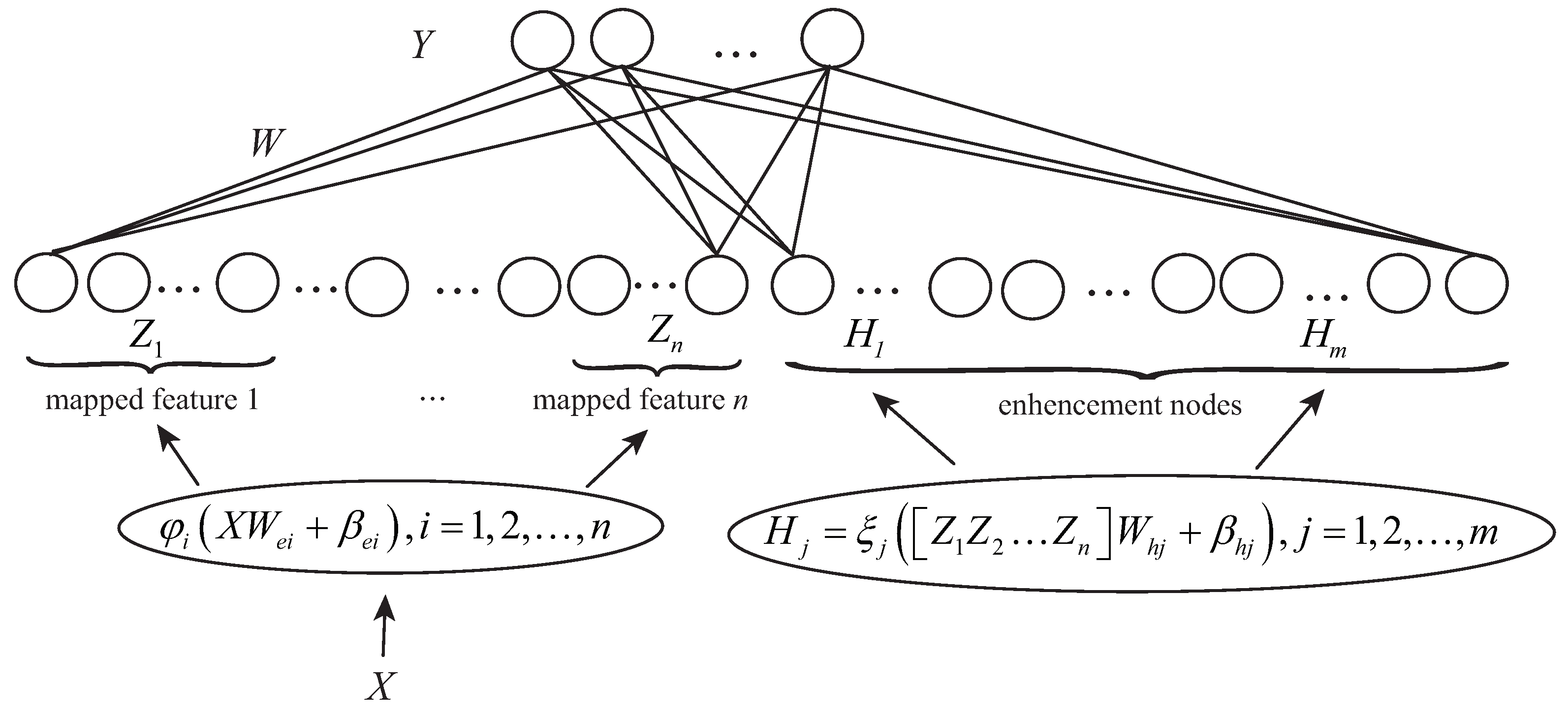
Then, we build the BNN model to depict this mapping relation. By collecting the data of $\Delta q_1,q_{10}$ and $\Delta q_2$, a sample set $(X,Y)$ is obtained to train the BNN model, where X is the input data including $\Delta q_1$ and $q_{10}$, Y is the output data only including $\Delta q_2$. The structure of the BNN model is shown in Figure 1.

The BNN model has n sets of the mapping feature nodes and m sets of the enhancement nodes. The output of the i-th group of the mapping feature nodes can be expressed as

$$Z_i={\phi }_i(X{W}_i^{mf}+{\beta }_i^{mf}),i=1,2,\dots ,n$$

(2)

where $W_i^{mf}$ and ${\beta }_i^{mf}$ are the weight and bias of the mapping feature nodes, respectively. ${\phi }_i$ is usually set as a linear transformation.

Letting $Z=[Z_1,\dots ,Z_n]$, the output of the j-th group of the enhancement nodes can be described as

$$H_j={\xi }_j(Z{W}_j^e+{\beta }_j^e),j=1,2,\dots ,m$$

(3)

where $W_j^e$ and ${\beta }_j^e$ are the weight and bias, respectively. ${\xi }_i$ is the activation function of the enhancement nodes, which can be set as Sigmoid function, Gaussian function, Tansig function, ReLU function and so on.

Letting $H=[H_1,H_2,\dots ,H_m]$, the output of the BNN model $\hat{Y}$ is

$$\hat{Y}=AW$$

(4)

where $A=[Z|H]$, $[Z|H]$ represents that Z and H are cascaded. W is the connecting weight of the BNN.

Different from other neural networks that employ the gradient descent method to obtain the network parameters, $W_i^{mf}$, ${\beta }_i^{mf}$, $W_j^e$ and ${\beta }_j^e$ in the BNN are randomly generated, and they do not need to be obtained by training. Thus, only W should be calculated, and it can be derived by the ridge regression approximation of the pseudoinverse [31], that is

$$\{\begin{array}{c}W=A^{+}Y\hfill \\ A^{+}=\underset{\lambda \to 0}{lim}{[\lambda I+A{A}^T]}^{-1}{A}^T\hfill \end{array}$$

(5)

where $\lambda$ is the ridge parameter, $A^{+}$ represents the pseudoinverse of A.

The training process of the BNN can be summarized as

Step 1: Set the numbers of the sets of the mapping feature nodes and enhancement nodes $n,m$. Meanwhile, set the activation function ${\xi }_j$.

Step 2: Randomly generate $W_i^{mf}$ and ${\beta }_i^{mf}$. Then, calculate $Z_i$ according to X and Equation (2). After that, let $Z=[Z_1,\dots ,Z_n]$.

Step 3: Randomly generate $W_j^e$ and ${\beta }_j^e$. Then, calculate $H_j$ according to Z and Equation (3). After that, let $H=[H_1,H_2,\dots ,H_m]$.

Step 4: According to Y and Equation (4), calculate W.

Through the above steps, the BNN model that accurately depicts the MCR between the passive linkage and the second linkage is established.

3. Solution of Target Angles

Figure 2 gives the schematic diagram of the PTUM, where the first joint is passive and the other two are active. In this figure, $q_n$ and $L_n$ ($n=1,2,3$), respectively, are the angle and length of the n-th linkage, and $(x,y)$ and $(x_d,y_d)$, respectively, are the position and target position of the manipulator end-point.

By means of coordinate transformation, the kinematic model of the PTUM is established as follows.

$$\{\begin{array}{c}x={\displaystyle \sum _{n=1}^3}(-L_n\sin {\displaystyle \sum _{m=1}^n}{q}_m)\hfill \\ y={\displaystyle \sum _{n=1}^3}(L_n\cos {\displaystyle \sum _{m=1}^n}{q}_m)\hfill \end{array}$$

(6)

Based on Equation (6), the position control of the PTUM can be translated into the angle control of all linkages. Therefore, firstly, we should get the target angle of each linkage in accordance with the target position of the end-point, which is the inverse kinematics solution of the PTUM. For a fully actuated manipulator, its inverse kinematics solution is easy to implement in many ways. However, the PTUM has a passive linkage, and the control of the passive linkage can merely be achieved by the MCR between the passive linkage and the second linkage. Therefore, the MCR depicted by the BNN model should be regarded as a constraint condition, and then fully considered in solving the inverse kinematics problem of the PTUM.

The PSO algorithm has the advantages of simplicity and fast convergence [32,33], so it is suitable for solving the inverse kinematics problem of the PTUM. Supposing there are C particles searching in D dimensional space, the updating equations of the PSO algorithm are

$$\{\begin{array}{c}{v}_{uv}^{i+1}=w{v}_{uv}^i+c_1{r}_1(p_{uv}^i-s_{uv}^i)+c_2{r}_2(p_g^i-s_{uv}^i)\hfill \\ s_{uv}^{i+1}=s_{uv}^i+v_{uv}^{i+1}\hfill \end{array}$$

(7)

where $v_{uv}^i$ and $s_{uv}^i$ are the velocity and position of the u-th particle in the v-th dimension, respectively. i is the number of iteration. w is the inertia weight. $c_1$ and $c_2$ are the learning coefficients. $p_{uv}^i$ and $p_g^i$ are the historical best position and the global best position of the u-th particle in i-th iteration, respectively. $r_1$ and $r_2$ are random numbers.

Then, using the following equation evaluates the calculation results.

$$f_e=\sqrt{{(x-x_d)}^2+{(y-y_d)}^2}$$

(8)

The process of the PSO algorithm is as follows:

Step 1: Stochastically initialize the assumed target angels of the passive linkage and third active linkage ${\tilde{q}}_{1d}$, ${\tilde{q}}_{3d}$.

Step 2: According to ${\tilde{q}}_{1d}$ and the start angle of the passive linkage $q_{10}$, the deviation $\Delta q_1$ is calculated by letting $\Delta q_1={\tilde{q}}_{1d}-q_{10}$. Taking $\Delta q_1$ and $q_{10}$ as the inputs of the established BNN model, the output of the BNN model is the rotation angle of the second linkage $\Delta q_2$. Thus, the assumed target angle of the second linkage can be calculated as ${\tilde{q}}_{2d}=\Delta q_2+q_{20}$.

Step 3: Substituting ${\tilde{q}}_{1d}$, ${\tilde{q}}_{2d}$ and ${\tilde{q}}_{3d}$ into Equation (6), the position of the end-point $(\tilde{x},\tilde{y})$ is obtained. Then, in accordance with Equation (8), $(\tilde{x},\tilde{y})$ and $(x_d,y_d)$, $f_e$ can be calculated. If $f_e<e_1$ ($e_1$ is a very small positive number), the target angle of the passive linkage is obtained, which is $q_{1d}={\tilde{q}}_{1d}$. Meanwhile, the target angles of the second linkage and third linkage are $q_{2d}={\tilde{q}}_{2d}$ and $q_{3d}={\tilde{q}}_{3d}$, respectively. Otherwise, update ${\tilde{q}}_{1d}$ and ${\tilde{q}}_{3d}$ according to Equation (7), and then jump to Step 2.

Through the above steps, the target angles of all linkages are obtained, which are $q_{1d}$, $q_{2d}$ and $q_{3d}$. Thus, the position control target of the PTUM can be fulfilled by controlling each linkage to rotate to its target angle.

4. Realization of Position Control Target

In the previous part, the target angle of each linkage is calculated. Then, by controlling each linkage rotates to its target angle, the end-point of the PTUM can be controlled from the given premier position to the given target position.

According to $q_{20}$ and $q_{2d}$, the rotation angle of the second linkage is $\Delta q_2=q_{20}-q_{2d}$. By controlling the second linkage rotates $\Delta q_2$, the passive linkage rotates $\Delta q_1$ due to the motion coupling between the second linkage and the passive linkage, and eventually stop at $q_1$ because of the friction at the joint. We define the deviation between $q_1$ and $q_{1d}$ as $\delta =q_{1d}-q_1$. Thus, the control target of the passive linkage is to make $\left|\delta \right|\le e_2$, where $e_2$ is a very small positive number. Once $\left|\delta \right|\le e_2$, the passive linkage is accurately controlled to its target angle through one rotation of the second linkage.

Considering that the third linkage is not adjacent to the passive linkage, the degree of coupling between the third linkage and the passive linkage is week. Thus, the rotation of the third linkage has few influences on the state of the passive linkage, so it can be ignored. Therefore, the third linkage is controlled to its target angle with low rotating speed when the second linkage rotates.

In this way, all linkages of the PTUM are controlled from their start angles to their target angles. Thereupon, the end-point of the PTUM is moved from its start position to its target position. Namely, the position control target of the PTUM is realized.

5. Experiments

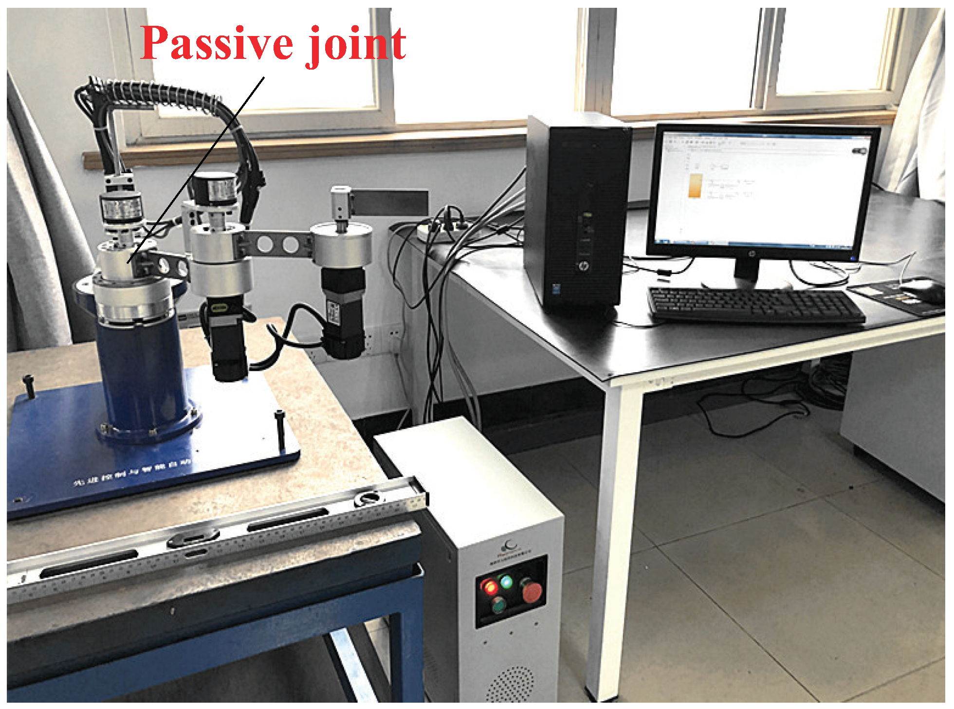
By locking the first joint of a planar 4-linkage underactuated manipulator with a passive second linkage all the time, we can obtain a PTUM with a passive first linkage, which is shown in Figure 3. Each joint of the PTUM equips an encoder used to measure the angle of the corresponding linkage. Moreover, both the second joint and third joint of the PTUM equip the servo motors working in the position control mode [34]. The motion control board sends the assembled data to the PC and sends the control commands to the servo motors. The length of each linkage is: $L_1$ = 0.158 m, $L_2$ = 0.154 m, and $L_3$ = 0.110 m.

5.1. Model Validation

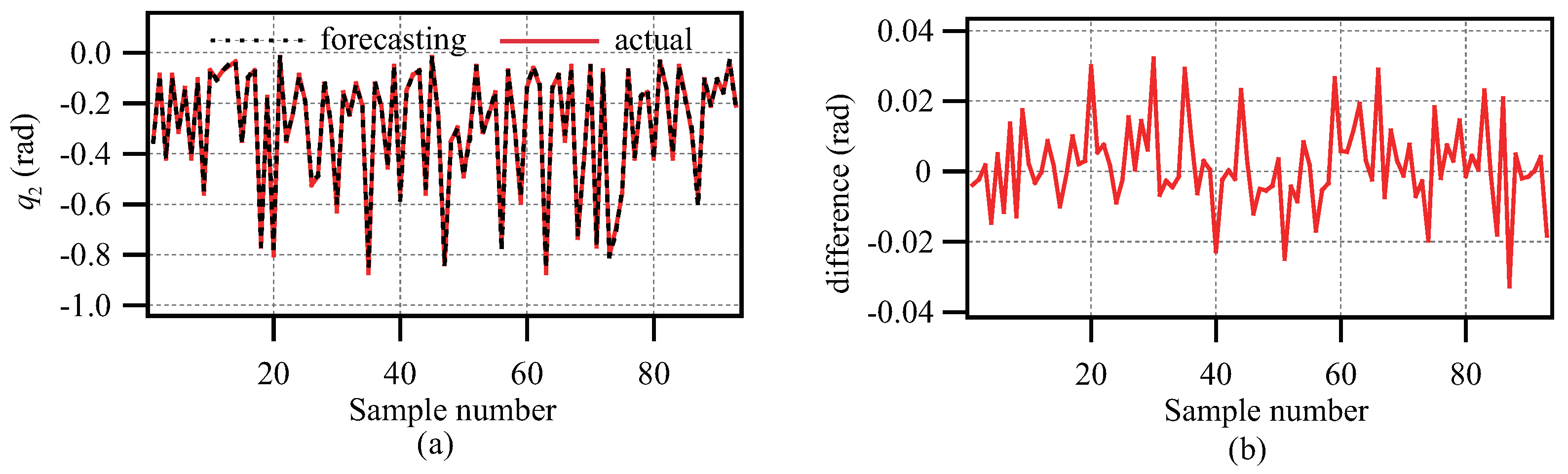
To establish and verify the BNN model that depicts the MCR between the passive linkage and the second linkage, 930 groups of data are collected, in which the training data accounts for 837 groups and the test data accounts for the remaining groups.

Here, using the following indexes evaluates the prediction ability of the BNN model [31].

$$RMSE=\sqrt{\frac{1}{L}\sum _{l=1}^L{(y_l-{\hat{y}}_l)}^2}\times 100\%$$

(9)

$$EC=1-\frac{\sqrt{{\sum }_{l=1}^L{(y_l-{\hat{y}}_l)}^2}}{\sqrt{{\sum }_{l=1}^L{(y_l)}^2}+\sqrt{{\sum }_{l=1}^L{(\hat{y})}^2}}\times 100\%$$

(10)

where $RMSE$ is the root mean square error, which is employed to reflect the size of the prediction error. $EC$ is the equalization coefficient, which is used to reflect the accuracy of the prediction. L is the total number of the samples. For the l-th sample, $y_l$ is the actual value obtained from the experiment, and ${\hat{y}}_l$ is the forecasting value calculated by the BNN model. When the RMSE value is smaller and the EC value is larger, the BNN model has the higher prediction accuracy and can describe the MCR between passive linkage and second one well.

The activation function ${\xi }_j$ is set as the Tansig function. Considering that there is no prior knowledge about the optimal values of m and n, we employ a trial-and-error method to explore their optimal values. By repeatedly training the BNN model with different values of m and n, we find that the optimal results are $m=49$ and $n=2$. Figure 4a shows the forecasting value and the actual value of the second linkage of the PTUM. Moreover, the deviation between the forecasting value and the actual value is shown in Figure 4b. The evaluation indexes of the BNN model are $RMSE=1.21\%$ and $EC=98.37\%$, respectively. Therefore, the established BNN model is effective and can be used to realize the position control target of the PTUM.

5.2. Experimental Results

Three groups of experiments are conducted to prove the validity of the presented control strategy. The parameters of the PSO algorithm are chosen as: $w=1$, $c_1=2$, $c_2=2$ and $e_1=1\times {10}^{-4}$. The rotating speeds of the second linkage and the third linkage are set as $\dot{q_2}=(5\pi /18)$ rad/s and $\dot{q_3}=(\pi /90)$ rad/s, respectively. Moreover, $e_{q_1}$ is chosen as 0.01 rad.

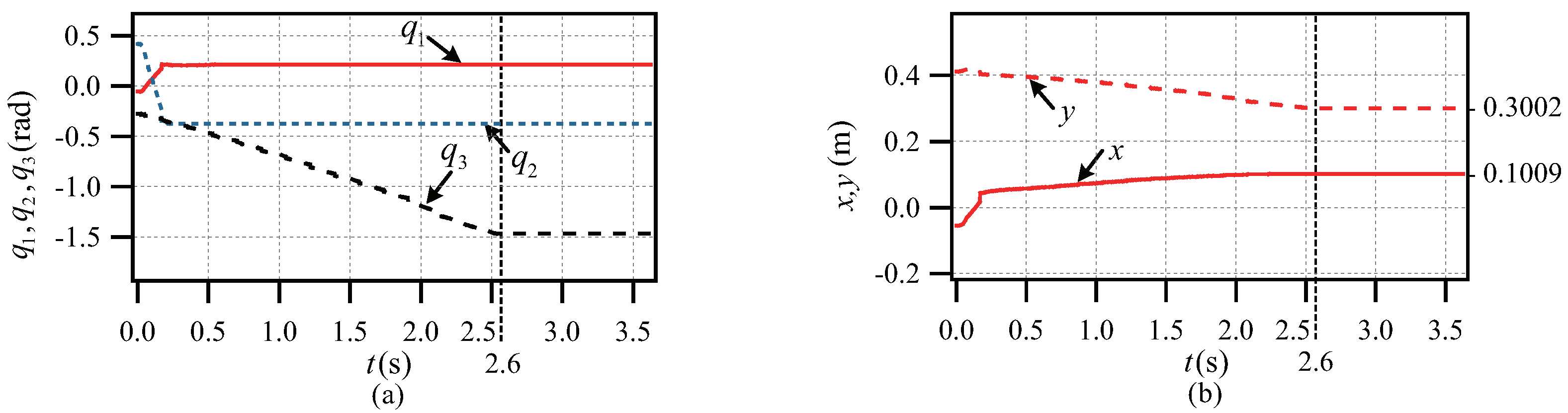
5.2.1. Case A

The target position and the start states of the PTUM are as follows

$$\{\begin{array}{c}[x_d,y_d]=[0.1000,0.3000]\mathrm{m}\hfill \\ [q_{10},q_{20},q_{30}]=[-0.0562,0.4180,-0.2746]\mathrm{rad}\hfill \\ [{\dot{q}}_{10},{\dot{q}}_{20},{\dot{q}}_{30}]=[0,0,0]\mathrm{rad}/\mathrm{s}\hfill \end{array}$$

(11)

According to Equation (11) and the established BNN model, the target angles of all linkages calculated by employing the PSO algorithm are $[q_{1d},q_{2d},q_{3d}]$ = [0.2206, −0.3743, −1.4656] rad.

The experiment results are shown in Figure 5. Based on $q_{20}$ and $q_{2d}$, we obtain $\Delta q_2$ = 0.7923 rad. By controlling the second linkage to rotate $\Delta q_2$, the passive linkage rotates $\Delta q_1$ = 0.2708 rad under the action of the coupling, and eventually stabilizes at $q_1$ = 0.2146 rad. According to $q_{1d}$ and $q_1$, we can get $\left|\delta \right|=0.0060\mathrm{rad}<e_{q_1}$, which shows that the passive linkage is accurately controlled to its target angle through one rotation of the second linkage. In addition, the third linkage is controlled to its target angle with low rotating speed ${\dot{q}}_3$ when the second linkage rotates. The position control target of the PTUM is fulfilled at t = 2.6 s. The end-point of the PTUM is stabilized at $[x,y]=[0.1009,0.3002]$ m. The absolute errors of the x-direction and y-direction are 0.009 m and 0.002 m, separately.

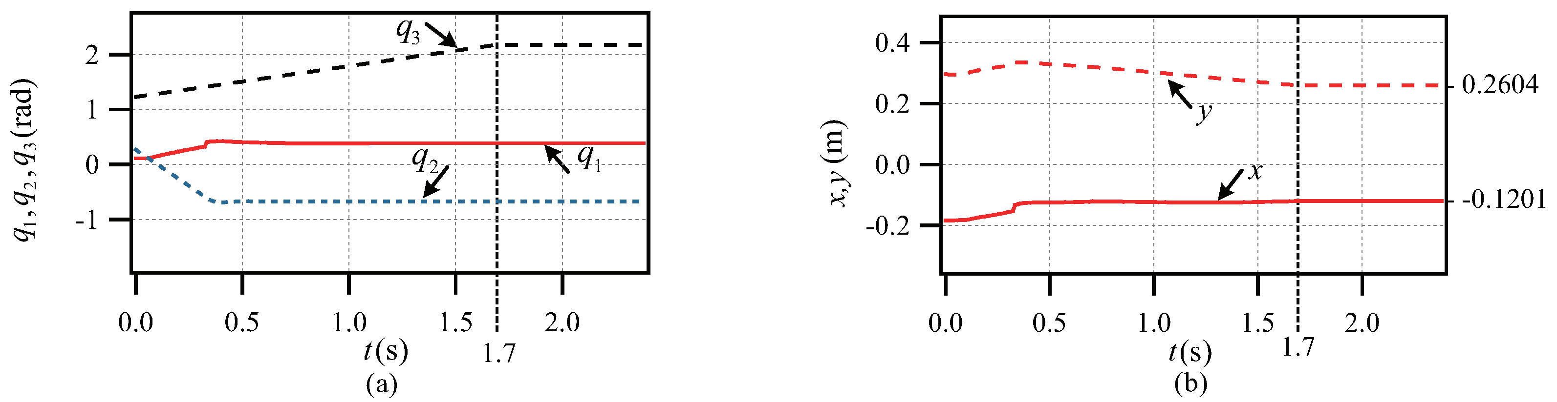
5.2.2. Case B

We perform the second group of experiments to further prove the availability of the presented control strategy. The start state and the target position of the PTUM are selected as

$$\{\begin{array}{c}[q_{10},q_{20},q_{30}]=[0.1053,0.2657,1.2261]\mathrm{rad}\hfill \\ [{\dot{q}}_{10},{\dot{q}}_{20},{\dot{q}}_{30}]=[0,0,0]\mathrm{rad}/\mathrm{s}\hfill \\ [x_d,y_d]=[-0.1200,0.2600]\mathrm{m}\hfill \end{array}$$

(12)

Similarly, according to Equation (12) and the established BNN model, the target angles of all linkages calculated by using the PSO algorithm are $[q_{1d},q_{2d},q_{3d}]$ = [0.3856, −0.6743, 2.1748] rad.

The experiment results are shown in Figure 6. It is light to find out that the control target is realized at t = 1.7 s. The end-point of the PTUM is stabilized at $[x,y]$ = [0.1201, 0.2604] m, and comparing the target position, the absolute errors are 0.001 m and 0.004 m, separately. It should be noted that the passive linkage is almost stationary after 1.5 s, but other linkages are still rotating. The reasons are as follows. The passive linkage can only be rotated through the coupling forces generated by the rotations of the active linkages. However, the passive linkage is also affected by the joint friction. When the coupling force is smaller than the joint friction, the passive linkage does not rotate.

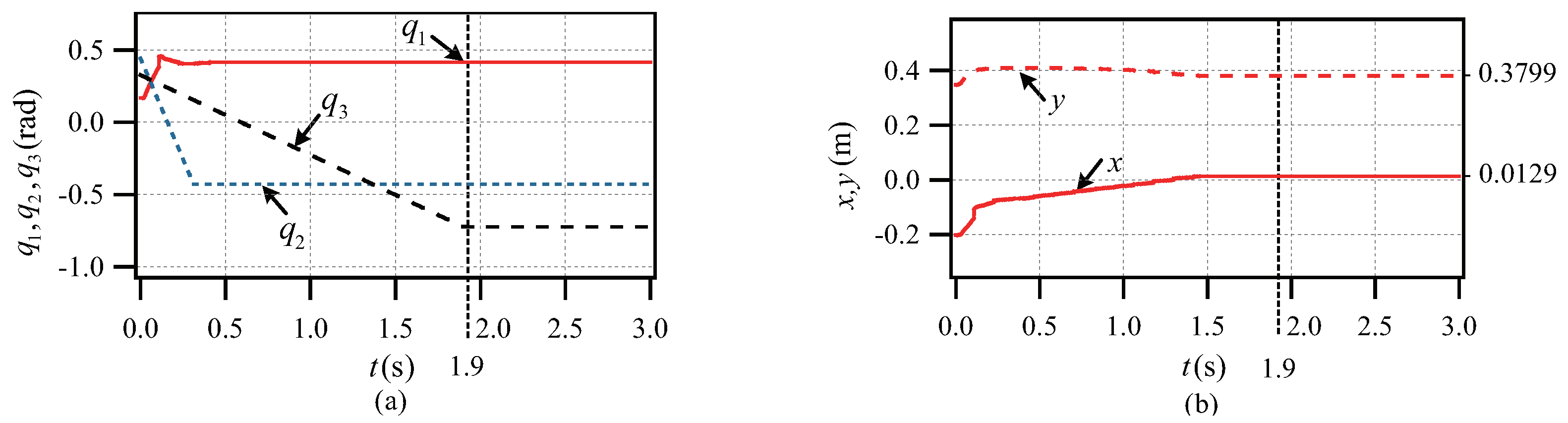
5.2.3. Case C

The start state and the target position of the PTUM in this group of experiments are chosen to be different from that of the first and second set of experiments, which are

$$\{\begin{array}{c}[q_{10},q_{20},q_{30}]=[0.1665,0.4413,0.3261]\mathrm{rad}\hfill \\ [{\dot{q}}_{10},{\dot{q}}_{20},{\dot{q}}_{30}]=[0,0,0]\mathrm{rad}/\mathrm{s}\hfill \\ [x_d,y_d]=[0.0120,0.3800]\mathrm{m}\hfill \end{array}$$

(13)

According to Equation (13) and the established BNN model, the target angle of each linkage calculated by using the PSO algorithm is $[q_{1d},q_{2d},q_{3d}]$ = [0.4159, −0.4286, −0.7240] rad. The experiment results are shown in Figure 7. The position control target of the PTUM is fulfilled at t = 1.9 s, and the end-point of the PTUM is stabilized at $[x,y]$ = [0.0129, 0.3799] m. Comparing the target position, the absolute errors of the position of the end-point are 0.009 m and 0.001 m, separately.

From the above three sets of experiments, we can find that the experiment results of the PTUM with a passive first linkage have realized a high precision if considering the inevitable systematic error. Hence, the presented control strategy is available.

6. Conclusions

This paper proposes the continuous control strategy in accordance with the BNN model for the PTUM with a passive first linkage to rapidly achieve its position control. Firstly, based on the collected experimental data, a BNN model is established, which can accurately depict the MCR between the second linkage and the passive linkage. Next, according to the start state of each linkage, the target position of the end-point and the established BNN model, the target angles of all linkages of the PTUM are calculated by using the PSO algorithm. On the basis of the start angle and target angle of the second linkage, its rotation angle is calculated. Through one rotation of the second linkage, the passive linkage is corporately controlled to its target angle. Meanwhile, the third linkage is controlled to its target angle with low speed. Eventually, three groups of control experiments prove that the presented control strategy is available and of great reference value.

References

- Beschi, M.; Villagrossi, E.; Tosatti, L.M.; Surdilovic, D. Sensorless model-based object-detection applied on an underactuated adaptive hand enabling an impedance behavior. Robot. Comput.-Integr. Manuf. 2017, 46, 38–47. [Google Scholar] [CrossRef]
- Chen, T.; Goodwine, B. Controllability and accessibility results for N-link horizontal planar manipulators with one unactuated joint. Automatica 2021, 125, 109480. [Google Scholar] [CrossRef]
- Ma, N.; Dong, X.; Axinte, D. Modeling and Experimental Validation of a Compliant Underactuated Parallel Kinematic Manipulator. IEEE/ASME Trans. Mechatron. 2020, 25, 1409–1421. [Google Scholar] [CrossRef]
- Huang, Z.; Lai, X.; Zhang, P.; Meng, Q.; Wu, M. A general control strategy for planar 3-DoF underactuated manipulators with one passive joint. Inf. Sci. 2020, 534, 139–153. [Google Scholar] [CrossRef]
- Oriolo, G.; Nakamura, Y. Control of mechanical systems with second-order nonholonomic constraints: Underactuated manipulators. In Proceedings of the 30th IEEE Conference on Decision and Control, Brighton, UK, 11–13 December 1991; Volume 3, pp. 2398–2403. [Google Scholar]
- Oriolo, G.; Nakamura, Y. Free-joint manipulators: Motion control under second-order nonholonomic constraints. In Proceedings of the IEEE/RSJ International Workshop on Intelligent Robots and Systems, Osaka, Japan, 3–5 November 1991; Volume 3, pp. 1248–1253. [Google Scholar]
- Lai, X.; Wang, Y.; Wu, M.; Cao, W. Stable Control Strategy for Planar Three-Link Underactuated Mechanical System. IEEE/ASME Trans. Mechatron. 2016, 21, 1345–1356. [Google Scholar] [CrossRef]
- Lai, X.; She, J.; Cao, W.; Yang, S. Stabilization of underactuated planar acrobot based on motion-state constraints. Int. J. Non-Linear Mech. 2015, 77, 342–347. [Google Scholar] [CrossRef]
- Zhang, P.; Lai, X.; Wang, Y.; Su, C.; Wu, M. A quick position control strategy based on optimization algorithm for a class of first-order nonholonomic system. Inf. Sci. 2018, 460–461, 264–278. [Google Scholar] [CrossRef]
- Suzuki, T.; Miyoshi, W.; Nakamura, Y. Control of 2R underactuated manipulator with friction. In Proceedings of the 37th IEEE Conference on Decision and Control, Tampa, FL, USA, 16–18 December 1998; Volume 2, pp. 2007–2012. [Google Scholar]
- Wang, Y.; Yang, H.; Zhang, P. Iterative convergence control method for planar underactuated manipulator based on support vector regression model. Nonlinear Dyn. 2020, 102, 2711–2724. [Google Scholar] [CrossRef]
- Bergerman, M.; Lee, C.; Xu, Y. Dynamic coupling of underactuated manipulators. In Proceedings of the International Conference on Control Applications, Albany, NY, USA, 28–29 September 1995; pp. 500–505. [Google Scholar]
- Akbarimajd, A.; Kia, S. NARMA-L2 controller for 2-DoF underactuated planar manipulator. In Proceedings of the 2010 11th International Conference on Control Automation Robotics Vision, Singapore, 7–10 December 2010; pp. 195–200. [Google Scholar]
- Duong, S.; Kinjo, H.; Uezato, E.; Yamamoto, T. Intelligent control of a three-DOF planar underactuated manipulator. Artif. Life Robot. 2009, 14, 284–288. [Google Scholar] [CrossRef]
- Li, Y.; Cao, Y.; Jia, F. A Neural Network Based Dynamic Control Method for Soft Pneumatic Actuator with Symmetrical Chambers. Actuators 2021, 10, 112. [Google Scholar] [CrossRef]
- Gong, M.; Liu, J.; Qin, A.; Zhao, K.; Tan, K. Evolving Deep Neural Networks via Cooperative Coevolution With Backpropagation. IEEE Trans. Neural Netw. Learn. Syst. 2020, 32, 420–434. [Google Scholar] [CrossRef]
- Song, Z.; Zhang, J.; Shi, G.; Liu, J. Fast Inference Predictive Coding: A Novel Model for Constructing Deep Neural Networks. IEEE Trans. Neural Netw. Learn. Syst. 2019, 30, 1150–1165. [Google Scholar] [CrossRef]
- Zhou, Y.; Zhang, L.; Yi, Z. Predicting movie box-office revenues using deep neural networks. Neural Comput. Appl. 2019, 31, 1855–1865. [Google Scholar] [CrossRef]
- Chen, C.; Liu, Z. Broad Learning System: An Effective and Efficient Incremental Learning System Without the Need for Deep Architecture. IEEE Trans. Neural Netw. Learn. Syst. 2018, 29, 10–24. [Google Scholar] [CrossRef]
- Zheng, Y.; Chen, B.; Wang, S.; Wang, W. Broad Learning System Based on Maximum Correntropy Criterion. IEEE Trans. Neural Netw. Learn. Syst. 2021, 32, 3083–3097. [Google Scholar] [CrossRef]
- Yang, F. A CNN-Based Broad Learning System. In Proceedings of the 2018 IEEE 4th International Conference on Computer and Communications, Chengdu, China, 7–10 December 2018; pp. 2105–2109. [Google Scholar]
- Peng, X.; Ota, K.; Dong, M. A broad learning-driven network traffic analysis system based on fog computing paradigm. China Commun. 2020, 17, 1–13. [Google Scholar] [CrossRef]
- Chen, C.; Liu, Z.; Feng, S. Universal Approximation Capability of Broad Learning System and Its Structural Variations. IEEE Trans. Neural Netw. Learn. Syst. 2019, 30, 1191–1204. [Google Scholar] [CrossRef]
- Hu, C.; Jain, G.; Zhang, P.; Schmidt, C.; Gomadam, P.; Gorka, T. Data-driven method based on particle swarm optimization and k-nearest neighbor regression for estimating capacity of lithium-ion battery. Appl. Energy 2014, 129, 49–55. [Google Scholar] [CrossRef]
- Tian, Z.; Su, S.; Shi, W.; Du, X.; Guizani, M.; Yu, X. A data-driven method for future Internet route decision modeling. Future Gener. Comput. Syst. 2019, 95, 212–220. [Google Scholar] [CrossRef]
- Momeni, A.; Maleki, S.; Khajeh, R. Analysts’ equity forecasts using of multi-layer perception (MLP). Adv. Environ. Biol. 2014, 8, 207–211. [Google Scholar]
- Kazem, A.; Sharifi, E.; Hussain, F.; Saberi, M.; Hussain, O. Support vector regression with chaos-based firefly algorithm for stock market price forecasting. Appl. Soft Comput. 2013, 13, 947–958. [Google Scholar] [CrossRef]
- Zhou, P.; Wang, C.; Li, M.; Wang, H.; Wu, Y.; Chai, T. Modeling error PDF optimization based wavelet neural network modeling of dynamic system and its application in blast furnace ironmaking. Neurocomputing 2018, 285, 167–175. [Google Scholar] [CrossRef]
- Sheng, B.; Li, P.; Zhang, Y.; Mao, L.; Chen, C. GreenSea: Visual Soccer Analysis Using Broad Learning System. IEEE Trans. Cybern. 2021, 51, 1463–1477. [Google Scholar] [CrossRef] [PubMed]
- Han, M.; Li, W.; Feng, S.; Qiu, T.; Chen, C. Maximum Information Exploitation Using Broad Learning System for Large-Scale Chaotic Time-Series Prediction. IEEE Trans. Neural Netw. Learn. Syst. 2021, 32, 2320–2329. [Google Scholar] [CrossRef]
- Ma, Y.; Liu, Z.; Chen, C. Hybrid spatial-spectral feature in broad learning system for Hyperspectral image classification. Appl. Intell. 2021. [Google Scholar] [CrossRef]
- Wang, D.; Tan, D.; Liu, L. Particle swarm optimization algorithm: An overview. Soft Comput. 2018, 22, 387–408. [Google Scholar] [CrossRef]
- Aydilek, I. A hybrid firefly and particle swarm optimization algorithm for computationally expensive numerical problems. Appl. Soft Comput. 2018, 66, 232–249. [Google Scholar] [CrossRef]
- Zhao, R. Design of Metro Locomotive Positioning Control System Based on Servo Motor Position Control Mode. Autom. Instrum. 2016, 5, 36–37. [Google Scholar]