Article

Introducing Twitter Daily Estimates of Residents and Non-Residents at the County Level

1
School of Public Administration, University of Central Florida, Orlando, FL 32801, USA
2
Geoinformation and Big Data Research Laboratory, Department of Geography, University of South Carolina, Columbia, SC 29208, USA
3
Department of Geosciences, University of Arkansas, Fayetteville, AR 72701, USA
*
Author to whom correspondence should be addressed.
Soc. Sci. 2021, 10(6), 227; https://doi.org/10.3390/socsci10060227
Submission received: 6 May 2021 / Revised: 31 May 2021 / Accepted: 10 June 2021 / Published: 14 June 2021

Abstract

:
The study of migrations and mobility has historically been severely limited by the absence of reliable data or the temporal sparsity of available data. Using geospatial digital trace data, the study of population movements can be much more precisely and dynamically measured. Our research seeks to develop a near real-time (one-day lag) Twitter census that gives a more temporally granular picture of local and non-local population at the county level. Internal validation reveals over 80% accuracy when compared with users’ self-reported home location. External validation results suggest these stocks correlate with available statistics of residents/non-residents at the county level and can accurately reflect regular (seasonal tourism) and non-regular events such as the Great American Solar Eclipse of 2017. The findings demonstrate that Twitter holds the potential to introduce the dynamic component often lacking in population estimates. This study could potentially benefit various fields such as demography, tourism, emergency management, and public health and create new opportunities for large-scale mobility analyses.

1. Introduction

Spatial mobility has long been a matter of interest for many disciplines (e.g., Faggian and McCann 2008; Squire 2010; Colleoni 2016), and particularly as a subject of study of geography (Cresswell 2011). In a context of unprecedented human movement, where short- and long-distance travel becomes more and more common, the study of all kinds of mobility is a necessity. The study of population movements has historically been severely limited by the absence of reliable data or the temporal sparsity of available data (Laczko 2015; Rango and Vespe 2017). For long-term movements (e.g., displacement, migration), census data, with a multi-year periodicity, and household surveys, often collected on an annual basis, constitute the main data source for studying population movements. Address registers, residence permits, and visa records have also been analyzed by researchers when available. However, in broad terms, changes of residence are rarely recorded and readily available at the time of the move, which precludes from connecting triggering events with population movements (Fussell et al. 2014). Shorter-term movements (e.g., commuting, vocational movements, or evacuations) need to rely on individual surveys or transportation statistics, which, in many cases, do not provide comparable information. The need for a comparable, reliable, and dynamic (with a finer temporal resolution) source of data is, therefore, a condition to improve our understanding of human spatial mobility.
In addition to the transportation revolution, advancements in electronics and computation have permitted us to reach a high degree of physical and virtual connectivity that Harvey (1989) named time–space compression. The digital revolution meant a shift from analog electronic technology to digital electronics, particularly after the propagation of the Internet and the mass production of computers and cell phones. In this digital era, the immense amount of data produced by the use of digital devices and web-based platforms is commonly referred to as “Big Data”, which many characterized as the “4+1 Vs”: Volume, Velocity, Variety, Veracity, and more recently, Value (Laczko 2015). Several researchers believe that Big Data holds the capacity to transform the study of spatial mobility (Isaacson and Shoval 2006; Billari and Zagheni 2017; Cesare et al. 2018). Within the great variety of Big Data types, geospatial digital trace data, also known as passive citizen sensor data, are seen as the source of data that can capitalize this change.
Our research seeks to develop a near real-time (one-day lag) Twitter census that gives a more temporally granular picture of local and non-local population at the county level. We aim to contribute to the field of digital and computational demography and obtain daily estimates of Twitter population stocks (residents and non-residents) at the county level for the whole contiguous US, as a first step for extending this analysis to other parts of the world. The implications of this research could mean the inclusion of a dynamic component in the study of population movements and serve as an input to model more sophisticated estimates of total residents (i.e., including other sources and variables to account for representation biases). Following this line of research, population estimates at a particular location and time can progress from scattered snapshots to a spatiotemporal continuum where authorities and researchers can track and measure population movements over time and across space at the daily and county scales. We believe the resulting output can potentially benefit several fields such as disaster management (e.g., tracking evacuations in real time), public health (e.g., gauging the compliance with travel restrictions), or tourism (e.g., determining the impact of cyclic and seasonal travel patterns) and help reach a better understanding of human mobility. To the best of our knowledge, this is the first attempt to produce an access-free variable of population estimates from passive citizen sensor data at high temporal (daily based) and spatial (county-based) scales, which can be implemented in population modeling.
The paper is organized as follows. First, we review common demographic approaches to the study of short-term and long-term population movements, followed by advances in the field of digital and computational demography, with a particular focus on previous contributions using geotagged social media. Next, we describe the data and methods applied to generate our results. The following section first deals with the internal validation of the residency assumption comparing the resulting data with self-reported home locations from Twitter users. We then conduct an external validation using annual aggregates of county residents and available statistics of SC 2% accommodation tax collections. Next, we present the potential of the results with a case study based on the 2017 total solar eclipse. Finally, we conclude with a discussion about the potential applications of the approach for different disciplines and further work.

2. Related Work

2.1. Measuring Population Movements through Traditional Sources: Censuses, Registries, and Surveys

Demography is a highly data-driven discipline that has sustained a significant share of its advancements in data collection efforts. Other disciplines with interest in studying population movements such as geography or tourism also share this concern about the availability of data to fuel their investigations. Many scholars have voiced the necessity of measuring population movements in a consistent manner considering all their dimensions, for which data quality is vital (Skeldon 2012; Bell et al. 2015). Monitoring populations is critical to evaluate demographic trends, and researchers have traditionally relied on a set of data sources that includes vital statistics, censuses/registries, and population-based surveys (Mallick and Vogt 2014; Fussell et al. 2017). However, Coleman (2013) pointed out that the distinction between these sources is becoming fuzzier and that hybrid approaches tend to be employed.
Demographers interested in large-scale population movements rely on censuses and registries to study these phenomena. Censuses and registries are systematic data collection efforts carried out by official entities to record information about a given population. Censuses are internationally accepted, and the United Nations issues standards and methods to assist national statistical authorities in their compilation (United Nations 2008). The main limitation of these approaches is their cross-sectional temporal coverage, with a considerable time lag between collection periods, which is insufficient for most migration research purposes (Fussell et al. 2014). Many countries only carry out censuses on a five- or ten-year basis. Some of the countries are systematic with these data collection procedures and undertake the census campaign on fixed years, therefore offering an inventory of the population of a territory on a regular basis. However, this is not the case for all countries, and many have abandoned or not initiated a regular and universal data collection strategy (Bell et al. 2015), which is often related to the considerable human and economic resources needed to carry out these initiatives (Fussell et al. 2014). Although demographers have used censuses to study migration, they are not explicitly designed for this purpose and can, therefore, only include a limited number of questions about this matter. Bell et al. (2015) discussed the different mechanisms used to infer migration/mobility data from censuses (i.e., lifetime migration, migration over a fixed interval, or place of the last residence), and stresses the great differences among countries, which further limits the comparability of the data.
Nationwide surveys are another widely used data collection method for internal migration and tourist movements. One of the main advantages over censuses or registries is that it can provide information with more temporal periodicity (more frequent data). In addition, national surveys can be tailored to reflect on large-scale migration, daily mobility, or tourist behaviors, unlike censuses and registries whose focus is not on these issues. This flexibility that surveys allow, in addition to being less expensive and involving considerably fewer human resources than censuses and registries, has enabled this data collection method to substitute universal data collection strategies (i.e., censuses and registries) in some countries (Franklin and Plane 2006). These surveys are normally available on a yearly basis, which is more amenable for migration studies, although it still does not suffice to comprehensively study short-term movements such as weekly/seasonal mobility patterns or special events such as emergency-induced population movements. One of the trade-offs of nationwide surveys (e.g., American Community Survey (ACS)) in comparison with census data is the loss of geographic detail (Bell et al. 2015). Annual surveys are not universal, which further generates problems of representativeness, particularly in small communities.
None of the traditional methods to keep track of population movements have shown to be completely adequate to study such dynamic and complex processes in a comparable manner, particularly in a context of increased spatial mobility. Thus, many scholars insist on incorporating innovative data collection methods that can complement conventional approaches and offer a more dynamic estimate of human spatial behavior (Willekens et al. 2016).

2.2. Digital Geospatial Shadow: An Opportunity

According to multiple researchers, the study of population movements and spatial behavior has entered a new era or a new data paradigm (Isaacson and Shoval 2006; Billari and Zagheni 2017; Cesare et al. 2018). These scholars refer to a new phase where the study of population movements can be much more precisely and dynamically measured using geospatial digital trace data. This new area of study has grown considerably in the previous few years, and a new field called digital and computational demography has emerged. Within this growing body of literature, many contributions have been made using different data sources and data collection approaches. The final output of these investigations has improved the knowledge of population processes, such as fertility and mortality (Tamgno et al. 2013), migration (Zagheni and Weber 2012), or emergency-induced population movements (Martín et al. 2020a).
Digital and computational demography is based on the use of Big Data to track populations. Within the term of Big Data, we find multiple types of data. The one that holds the greatest potential for the field is geospatial digital trace data. These, also known as passive citizen sensor data, are generated by individuals in their daily digital activity. Passive citizen sensor data can be used for many purposes, with research being just one of them. These digital shadows, unintentionally left behind by the individuals, can be used to determine the spatial behavior of those who generated them, as some carry information about the physical location where the data record was created. The possibilities of these data go beyond their application in demography (e.g., Zagheni et al. 2014), and other fields or disciplines have also leveraged them. This is the case of transportation (Jurdak et al. 2015), public health (Wesolowski et al. 2012), sociology (Amini et al. 2014) or natural hazards (Martín et al. 2017; Li et al. 2018; Huang et al. 2018, 2019). Some of the characteristics that these researchers seek in passive citizen sensor data are its immediacy, as its collection and exploitation can be carried out close to real time, its wide coverage, and its reduced cost (Spyratos et al. 2018).
Among the different sources of passive citizen sensor data, mobile phone call detail records (CDR) have been the one with the largest number of applications. The application of CDR in short-term mobility and human spatial behavior studies has been extensive. For instance, Wesolowski et al. (2014) looked into the mobility patterns and connectivity in West Africa to monitor the progression of the 2014 Ebola outbreak and predict its future spread. This data source also has been proved valid in other contexts such as earthquakes and humanitarian crises. An illustration of this is found in Bengtsson et al. (2011), where this team developed a methodology to detect population movements leading to cholera outbreaks by mining call data records in the aftermath of the Haiti earthquake in 2011, concluding that the method was able to correctly estimate population movements during disasters and outbreaks. However, contrary to short term studies of population movements, long-term analyses using CDR are not common. One of the few studies in the literature was conducted by Blumenstock (2012), who investigated a four-year dataset from 1.5 million Rwandans and revealed patterns of temporary and circular migration previously unknown. The main limitation is data accessibility, as these data are privately owned by corporations that are reluctant to freely share these data for research purposes. In addition, if access to the data is ever granted, it is after extensive paperwork and bureaucracy, precluding the use of these data in real-time applications. Additionally, scholars have voiced concerns about ethical and privacy issues, in particular with vulnerable populations (Taylor 2016). Despite these pitfalls, CDR is considered one of the richest passive citizen sensor data, as the penetration of cell phones in today’s society is very high (Turner 2020), and they provide high periodicity data (continuous records rather than sporadic or episodic). WiFi and Bluetooth networks are another rich data source for spatial mobility, and even though they share the difficulty of data accessibility with CDR, they have been explored to track population movements at smaller scales (i.e., neighborhood) and indoor settings. Thus, for instance, Traunmueller et al. (2018) were able to analyze human mobility trajectories in New York City using WiFi probe data.
Due to the difficulty of accessing mobile phone call records or WiFi and Bluetooth networks, many researchers have resorted to other sources of digital shadows to track populations. Some of the platforms explored by researchers include video conference applications. Using Google+, Messias et al. (2016) developed a method to measure aspects such as migration clusters of country triads that were beyond the reach of traditional demographic sources, while leveraging Skype, Kikas et al. (2015) found that the percentage of international calls and foreign logins in a country can be used as relatively accurate proxies for estimating migration. LinkedIn data allowed Barslund and Busse (2016) to determine that the European Union is losing tech skills as Information Technology professionals are leaving towards the United States. Social media, and particularly Twitter, is considered the richest supplier of data due to the easier accessibility of its content (Stock 2018). Although Facebook has a more restrictive policy when it comes to data sharing and exploitation for mobility and migration purposes, several authors have been able to obtain positive results with this data source. For instance, Zagheni et al. (2017) managed to estimate stocks of migrants within and across countries using Facebook’s advertising platform. More recently, and using the same platform, Alexander et al. (2019) estimated a 17.0% increase in the number of Puerto Rican migrants in the continental United States in the months after Hurricane Maria.
Because of its open data sharing policy, Twitter data are the most broadly used and have garnered a lot of attention from researchers, including migration and mobility scholars. Twitter data offer immediacy (i.e., data available almost in real-time) and adequate spatiotemporal coverage for many mobility and migration analyses. Its reduced cost—mainly only computational—and a large number of users in many countries are also seen as great advantages for research and management. Many fields have mined Twitter data for research purposes: psychology (Bittermann et al. 2021), tourism (Ćurlin et al. 2019), urban studies (Roberts et al. 2019), sociology (Tinati et al. 2014), geography (Takhteyev et al. 2012), journalism (Sheffer and Schultz 2010), emergency management (Martín et al. 2017), public health (Bisanzio et al. 2020; Li et al. 2021a), or even medicine (Pershad et al. 2018). Within this myriad of studies, several authors have focused on using Twitter to estimate human mobility, whether it is under normal circumstances or triggered by an extraordinary event. Among those who studied human mobility and migration not connected to triggering events, Hawelka et al. (2014) were able to estimate the volume of international travelers by country of residence and their mobility profile, analyzing a pool of almost a billion tweets from 2012 and computing radius of gyration for each user. Zagheni et al. (2014) used geolocated tweets from 500,000 users in a 2-year period and highlighted that Twitter is a valid data source to predict turning points in migration trends and to improve understanding of the relationships between internal and international migration. Among those interested in spatial mobility following extraordinary events such as emergencies, Wang and Taylor (2016) revealed spatiotemporal patterns of human mobility analyzing a 2-year Twitter sample and calculating individual displacements (distance over two consecutive points from one individual), concluding that mobility in urban environments is altered during disaster events and this disturbance depends on the characteristics of the emergency. Martín et al. (2017) measured evacuation compliance in South Carolina during Hurricane Matthew by tracking Twitter users through their geotagged tweets during different stages (pre, during, and post emergency), which was later extended by Jiang et al. (2019), focusing on the users’ social networks, activity spaces, and sentiment. Similarly, this method was also used to estimate post-disaster migration following Hurricane María in Puerto Rico in 2017 (Martín et al. 2020b). In the context of the COVID-19 pandemic, Huang et al. (2020), measuring two types of distance—single-day distance and cross-day distance—revealed that mobility patterns obtained from Twitter data are amenable to quantitatively reflect the mobility dynamics, finding country discrepancies in the response throughout the different epidemic phases.
This study aims to take a step further and develop an automated algorithm that converts millions of daily geotagged Twitter data into an easily understandable measure of resident and non-resident stocks, thus introducing a dynamic component in the measure of spatial mobility. Most of the research projects cited earlier, and many others, focus on relatively small regions, short periods of time, and are based on particular events (e.g., a hurricane), having to download, pre-process (i.e., data cleaning), and analyze the data for each set of conditions, which is time and resource consuming and makes comparisons between different studies very challenging due to differences in the methodologies. The research presented here offers much-needed information in several fields such as tourism, epidemiology, or emergency management; this is a rapid, comparable, and geospatially detailed product of population estimates that can be directly implemented as a dynamic input in more sophisticated population modeling approaches.

3. Materials and Methods

3.1. Case Study

The 2017 US Solar Eclipse offers a great opportunity to test the potential of our approach to detect, quantify, and compare the influx of Twitter non-residents (hereinafter referred to as visitors) to counties within the path of totality and to counties outside the path of totality (see Figure 1). On Monday 21 August 2017, a total solar eclipse moved across the continental US from the northwest (Oregon) to the southeast (SC). Millions of people traveled nationally and internationally to see the astronomic event. Some have pointed out this was the “greatest temporary mass migration of humans” in US history, which put major pressure on infrastructures as nearly 200 million people lived a one-day drive from the totality path, with SC being the closest location for near 95 million of them (Zeiler 2017). Many cities and towns across the path of totality saw their population multiplied, many accommodations were 100% booked months in advance, and many roads experienced bumper-to-bumper traffic during the previous weekend and on the day of the Eclipse (Boyle 2017). As we can see in Figure 1, the path of totality covered nearly half of SC in a 70-mile-wide swath and across the US. Thus, if our method is operatively valid, we can expect a major influx of visitors in the counties under the totality path and a smaller increase in the counties outside of it.

3.2. Classification of Daily Residents and Non-Residents

Over 1.5 billion (N = 1,527,455,625) geotagged Twitter data were collected using the Twitter Streaming Application Programming Interface (API) covering the contiguous US from 2017 to 2019. The tweets were cleaned and preprocessed into CSV (comma-separated values) files, stored in a big data computing cluster. Apache Hive, Impala, and GIS Tools for Hadoop by Esri were used to conduct spatial analyses and query analytics (Li et al. 2021c).
The literature provides several methods to classify users into local (resident) users and non-resident users. Some have used density-based spatial clustering of applications with noise (DBSCAN) (Ester et al. 1996) to retrieve the user’s home location (Huang and Xiao 2015), which is the most precise method to obtain the home location at the finest possible spatial resolution when the geolocation is based on a pair of coordinates (latitude and longitude). However, the scope of our research is focused on the county level, which includes tweets with a spatial resolution finer than county (e.g., a city name) but that is not necessarily pinpointed with a pair of coordinates. Others have based their home location classification in the study of the center of mass (Hawelka et al. 2014) or the median center (Martín et al. 2017), which is in accordance with the findings of Jurdak et al. (2015) about the preference of people to tweet around half of the time from their most popular location (home location). Following this idea, another method to identify the residency of users has involved weighting the most frequently visited cluster (Lin and Cromley 2018) or just selecting their most repeated location (the mode in numerical terms) (McNeill et al. 2017). Different scenarios and conditions have been applied to this latter approach, including n-day time intervals (Jiang et al. 2018; Hu et al. 2019) or night-time tweets (Koylu 2018). Unfortunately, these investigations often do not report a measure of the goodness of their home location assumptions (validation), for which selecting the most appropriate method remains conditional to the objectives of the particular research project.
For this reason, we adopted the most repeated location among the tweets sent by each individual user during a whole year (e.g., 1 January 2017–31 December 2017). In addition, we tested n-day time interval, but the small change in the residency assumptions (between 2% and 5%) led us to use the most simplistic approach based on just the most repeated location. The workflow to obtain the total Twitter residents and non-residents per county per day for the contiguous US is presented below.
(1)
For each day, for each county of the contiguous US, obtain a list of distinct (unique) users active in that county.
(2)
Retrieve all tweets available in our repository from each of the active users from the year of the study period. We used an entire year to eliminate the effect of seasonal variations had we chose a shorter timeframe.
(3)
Assign a distinctive code of the US county, or country if outside the US, from where each of the tweets was sent.
(4)
Compute the most repeated tweeting location for each user during the year of the study period.
(5)
Classify those whose most repeated tweeting location falls within the analyzed county as residents. If a user’s most repeated tweeting location is outside of the county, the program classifies this user as a non-resident. A third category, unknown, is reserved for those users whose most repeated tweeting location cannot be calculated (when having less than two tweets in the whole year, or more than one county as the most repeated tweeting location).
A program was developed to perform the tasks in the workflow to automatically compute the daily number of users (resident, non-resident, and unknown) from billions of tweets for each county of the contiguous US for the whole year of 2017, 2018, and 2019.
To facilitate the mapping and comparison across the different counties, we standardize the classified daily residents and non-residents for each county along the year using Equation (1).
z i j = x i j x j ¯ S j
where z i j denotes the residents (or non-residents) standard score for county j on day i. x i j denotes the estimated residents (or non-residents) for county j on day i. x j ¯ denotes the mean of estimated residents (or non-residents) for county j along a year, and S j denotes the standard deviation of the estimated residents (or non-residents) for county j along a year.

3.3. Validation

To evaluate the performance of our automated classification, we designed two validation analyses—internal and external—using the SC as the study area. In addition, we use the 2017 Solar Eclipse of 21 August as operational validation to show the potential of the method, using South Carolina and the contiguous US as the study areas.

3.3.1. Internal Validation: Residency Assumption

The internal validation is designed based on the self-reported home location of a sample of Twitter users. Using self-reported home location is a common strategy to determine the residence of the social media user. For instance, according to Zagheni et al. (2018), this is the approach followed by Facebook Adverts Manager to define expats (people whose original country is different from the current country). The process is summarized in the following steps: (1) Extraction of a representative sample of users. We calculated the total number of distinct active Twitter users (who tweeted at least once) in 2017 in SC. A total of 190,608 distinct users were identified. We randomly selected a significant sample size of these population of Twitter users with a confidence level of 99% and a margin of error of 5%. The sample size was therefore fixed in 661 Twitter users with self-reported home location. (2) Manual assessment of the self-reported home locations of the sampled users to eliminate obvious fake locations (e.g., “Neverland”, “Waffle House”, “Mars”, or “Moon”) or not geographically detailed enough descriptions to estimate the home location at the county level (e.g., “South Carolina” or “United States”). A total of 18.2% of the initial sample reported fake locations, while 22.0% did not provide enough geographical detail. We randomly substituted these users with other users whose self-reported location was not fake and accurate enough until obtaining 661 users. (3) Manual attribution of a county from the self-reported location for each validation user. For instance, if a user self-reported their home location as Columbia, SC, we assigned Richland County. (4) Comparison of automatically estimated home location based on the most repeated tweeting county (mode) and the validation sample (failure/success analysis). (5) Individual assessment of the misidentifications.

3.3.2. External Validation of Final Estimates

The second validation assessment aims to relate the obtained results with the most accurate and spatiotemporally detailed data about the number of residents and tourist activity through a case study.
We used 5-year ACS estimates to relate the annual number of distinctive users per county with county resident estimates for 2017. The ACS is an annual survey of the U.S. Census Bureau designed to supplement the decennial census. There are no official statistics about the daily or seasonal variations in resident populations. Therefore, our daily data had to be aggregated to annual totals in order to be compared with ACS data. For tourism statistics, the only data available at the county level for SC are the monthly state accommodation tax (SCPRT 2019), which is a mandatory 2% charge applied to all accommodations statewide. Accommodations are defined as “the rental or charges for any rooms, campground spaces, lodgings, or sleeping accommodations furnished to transients by any hotel, inn, tourist court, tourist camp, motel, campground, residence, or any place in which rooms, lodgings, or sleeping accommodations are furnished to transients for a consideration” (SCPRT 2019). Again, there is no official data available at the daily level, and our daily estimations had to be aggregated, in this case to monthly data. We are aware that the state accommodation tax is just a partial estimate of the non-resident movements, as it does not register trips that do not involve accommodation or those who spend the night at second homes or relatives’/friends’ homes.

4. Results

4.1. Internal Validation of Residency Assumption

One of the objectives of the internal validation was to determine whether a threshold about the minimum number of tweets from users in the previous year was needed in order to accurately identify their home location. In Table 1, we report the percentages of successful identification of home residency by our method (most repeated tweeting county or mode) in comparison to the user’s self-reported home location. As we can see in the table, once assigned the home location category “unknown” to those whose most repeated tweeting county location could not be calculated, the percentage of success (between 77 and 78%) is almost independent from the number of tweets per user per year for users with less than 200 tweets. Only for users with 200 tweets or more in the year (26.2% of the total users) the home location identification slightly improves by roughly 5%. For this reason, we decided not to apply any threshold in our method (all users).
We believe 77–78% of successful home location identification is sufficiently accurate for an automated method, even more so after individually analyzing the misidentifications (which brings the accuracy to 83.1%). Looking at the home location identification failures of users in the category “All users” from Table 1 (no threshold applied), we found out that 37 of the misidentifications (26%) could be related to the user identifying themselves as a resident of a multicounty metropolitan area or with Twitter inaccurately placing a geotag (place) in a county that does not belong there. Table 2 shows these issues, which relate to the validation process, and that might make the percentage of successful home-identification be lower. In the case of Fulton and Gwinnett (GA), the user identified themselves as an Atlanta (GA) resident; however, most of their tweeting activity falls within Gwinnett County, part of the metropolitan area of Atlanta. This problem was also common in the Charleston (SC) and Columbia (SC) metropolitan areas. For instance, our method assigned home location in Berkeley or Dorchester (in towns such as Summerville, Goose Creek, or Hanahan) to users who self-reported Charleston as their home location. This is particularly relevant in the SC capital city, Columbia, where the Congaree River divides the metropolitan area into two counties (Richland and Lexington) and multiple cities (Columbia, West Columbia, Cayce, or Lexington). Thus, 10.4% of the home location misidentifications occurred in this area, where the user self-reported to be a resident of Columbia (Richland County), but their tweeting behavior showed their home residence in places such as West Columbia, Cayce or Lexington (Lexington County). Similarly, this issue was also observed in the counties of Greenville and Pickens, where the users would self-report Greenville as their home location but their tweeting behavior would show that their home residency (most repeated tweeting location) is in the metropolitan area (partly pertaining to Pickens County). Finally, we also identified how Twitter wrongly placed the town of Fort Mill (SC) in Lancaster County, when it is located in York County. This error transfers into an automated home location identification and is external to our identification approach. Speculating that the 37 misidentifications (32 from metropolitan areas issues and 5 because of the Twitter geolocation of Fort Mill) were actually successful home location identifications, the percentage of success reported in Table 1 would increase from 77.3% to 83.1%.

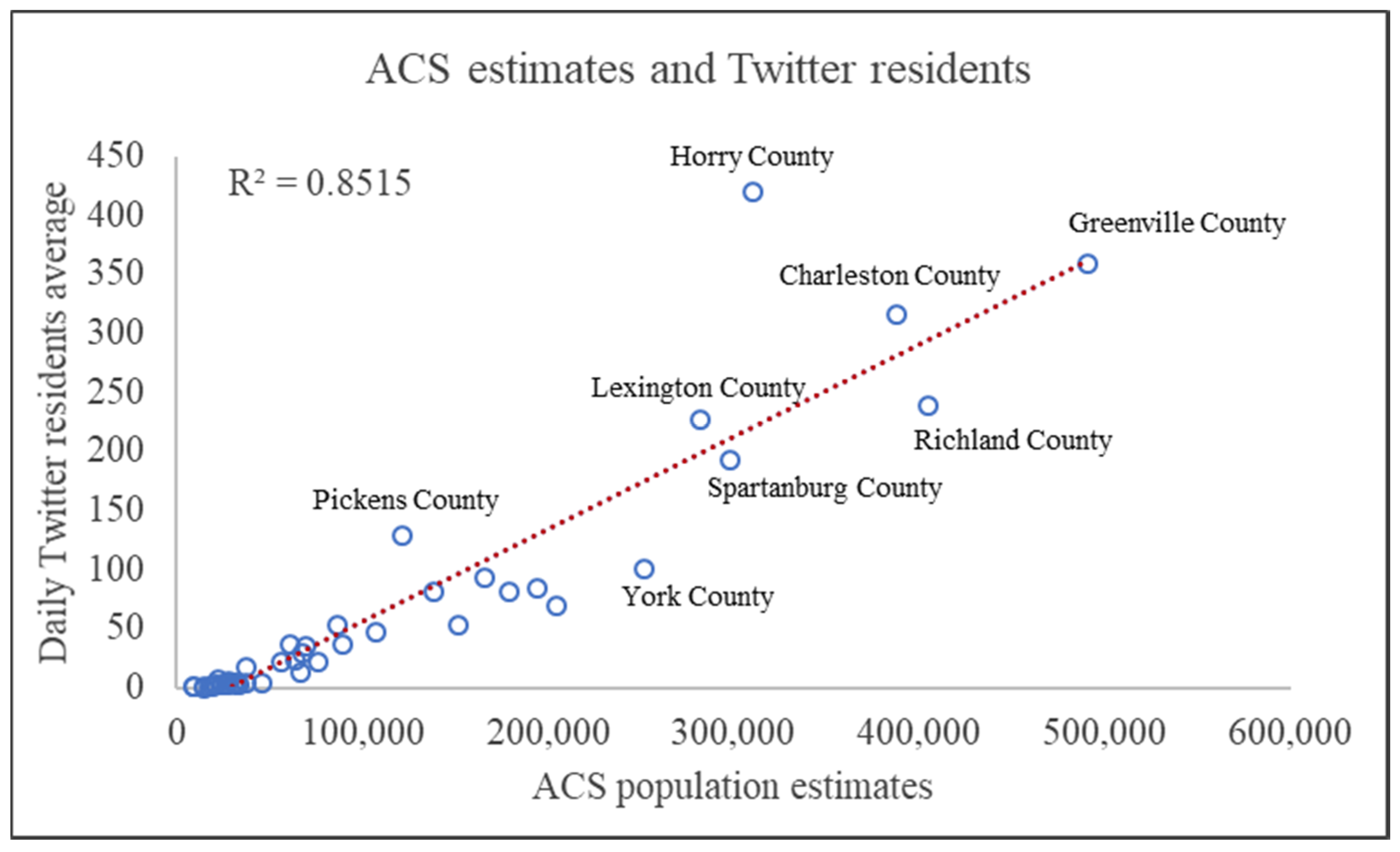
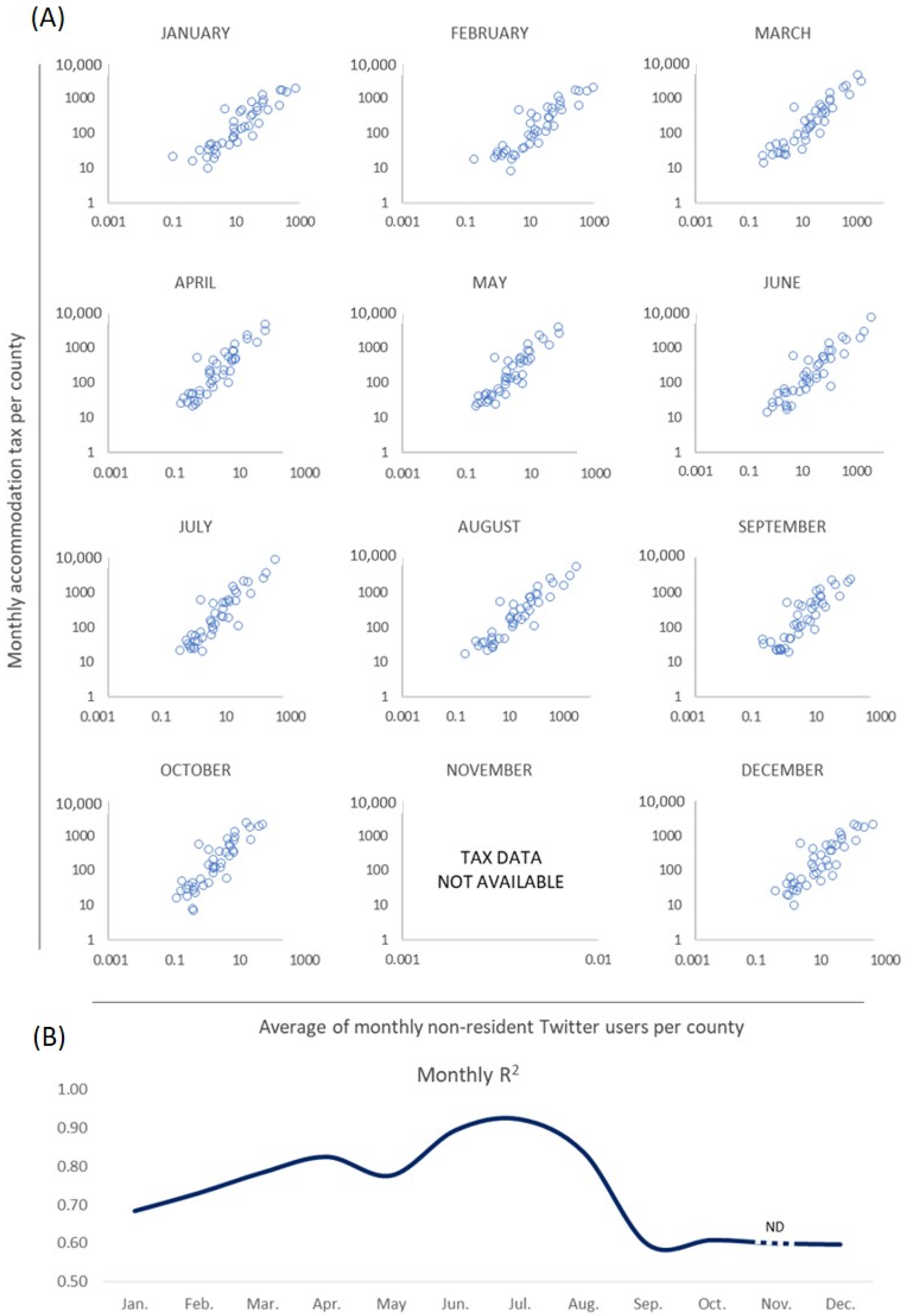
4.2. External Validation of Final Estimates

Here, we present the relationship of our Twitter classification of residents and non-residents with the most spatiotemporally detailed official statistics. Figure 2 shows the association between the estimated total county population and the daily average of total active Twitter residents per county. As we can see, the annual average of daily Twitter residents is highly correlated with the ACS estimates, and 85 percent of the variability in the data is explained by a straight line through the observations. We only identified one big outlier corresponding with Horry County (Myrtle Beach area), for which we have no explanation at this time. The rest of the observations are close to the line, confirming that more Twitter residents are found in more populated counties.
Figure 3 relates the monthly aggregated observations of non-resident Twitter users with SC Statewide 2% Accommodations Tax Collections. In the monthly log-log plots, we can observe there is a strong positive linear relationship between the two variables. The R2 values further reveal a closer relationship during the months of highest accommodation occupancy (summer months), with around 90% of the variance of June and July explained by a straight line. We believe the lower values during the rest of the months (still with strong relationships with R2 over 0.6) are explained by the difference in travel behavior. During the low (touristic) season, from September to February, travels tend to be more locally based and of shorter duration, not reflecting as much on accommodation occupancy as much of this travel is day-long trips or the local SC population with second homes in touristy areas (e.g., Myrtle Beach). The SC Department of Parks, Recreation, and Tourism did not have available data of accommodation tax collections for November 2017.
Overall, we are aware that the nature of the official data used for the external validation (ACS annual resident estimates and monthly aggregates of accommodation tax collections) does not fully confirm the goodness and fit of our approach. While these data constraints hinder the assessment of a geotagged social media approach to provide a daily picture of the behavior of residents and non-residents at the county level, they reveal the necessity of research of this kind that offers innovative solutions to the paucity of data about population stocks and mobility in such a spatiotemporally detailed scale.

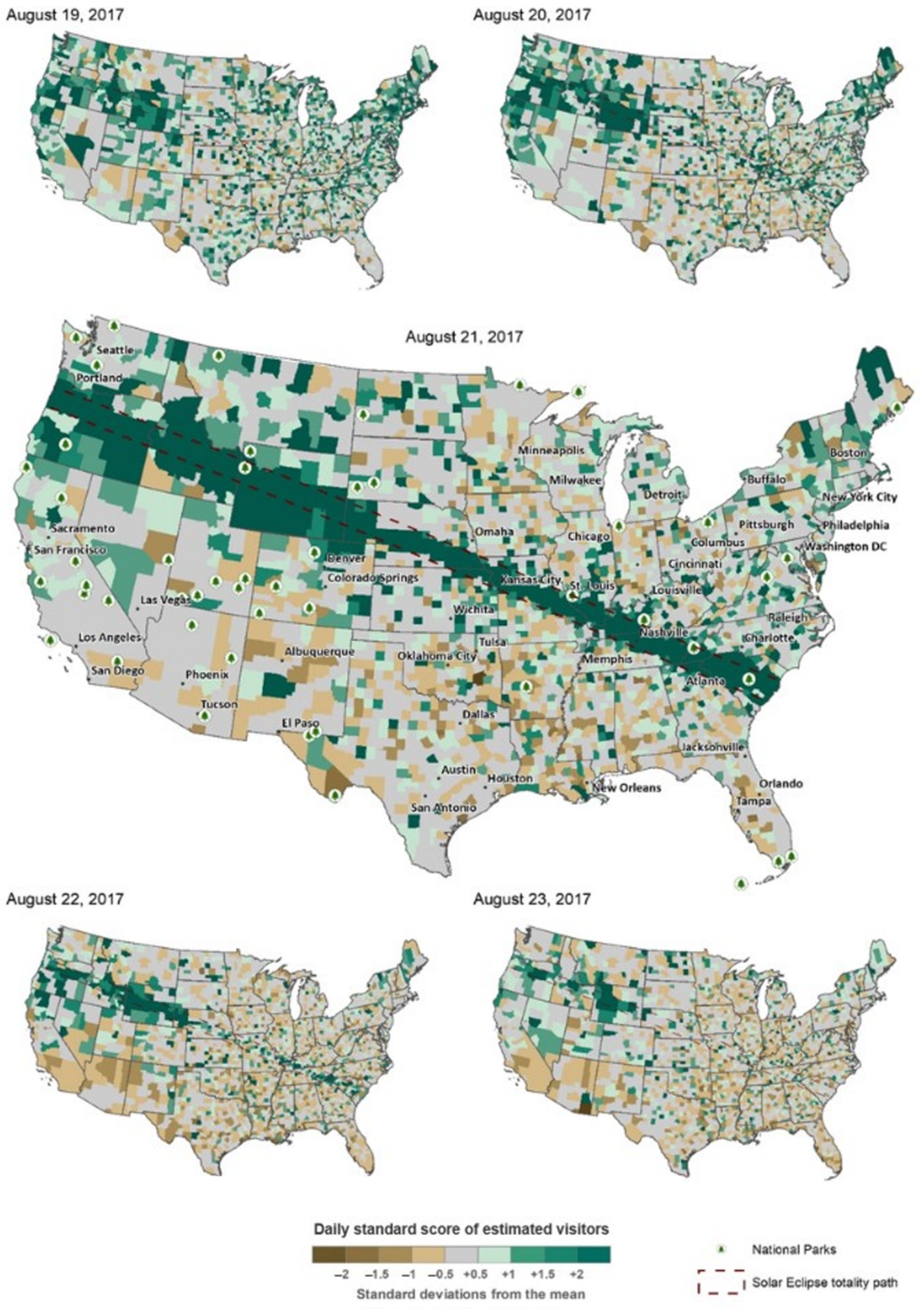
4.3. Case Study: Visitor Dynamics during the 2017 US Solar Eclipse

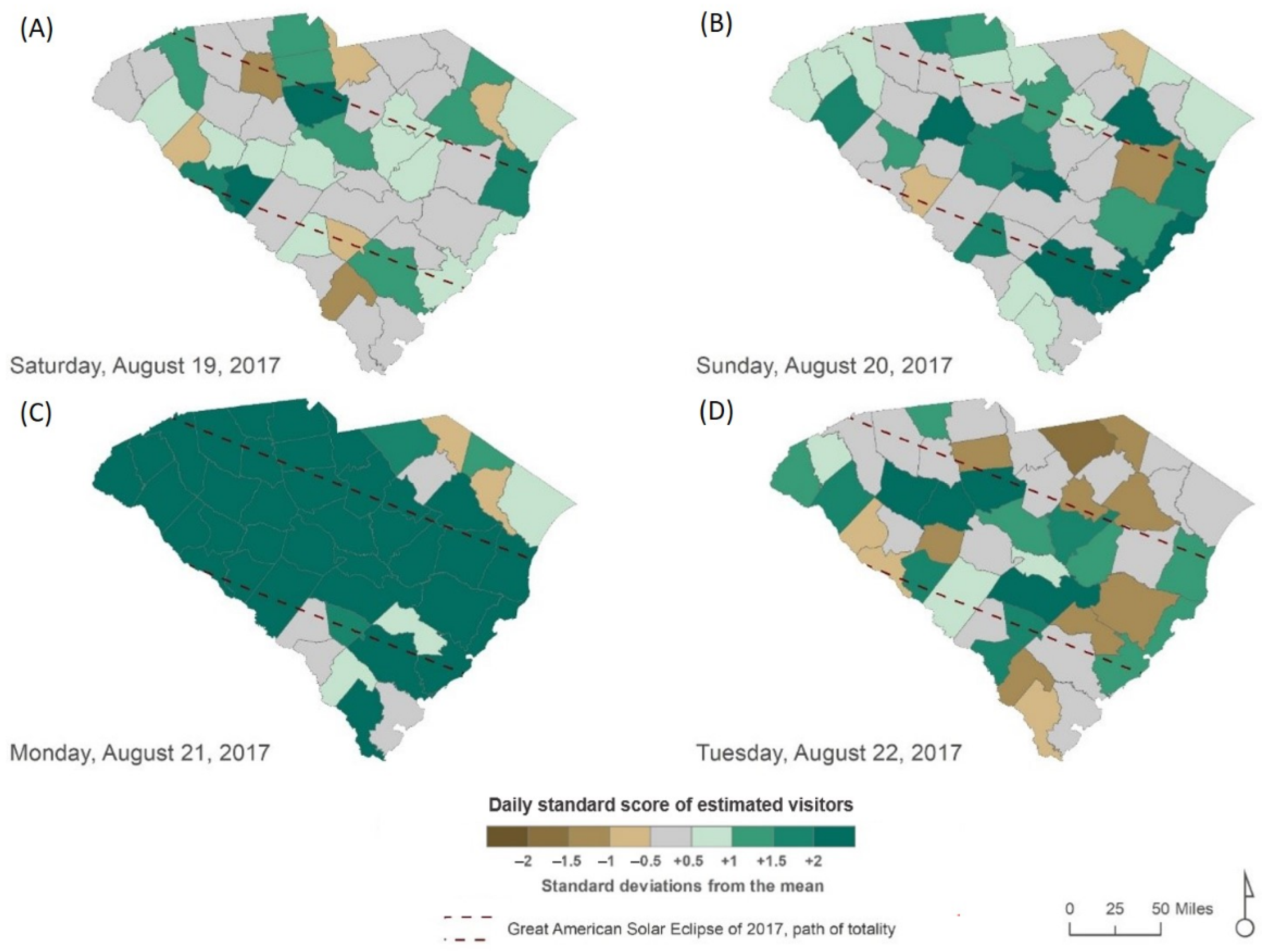
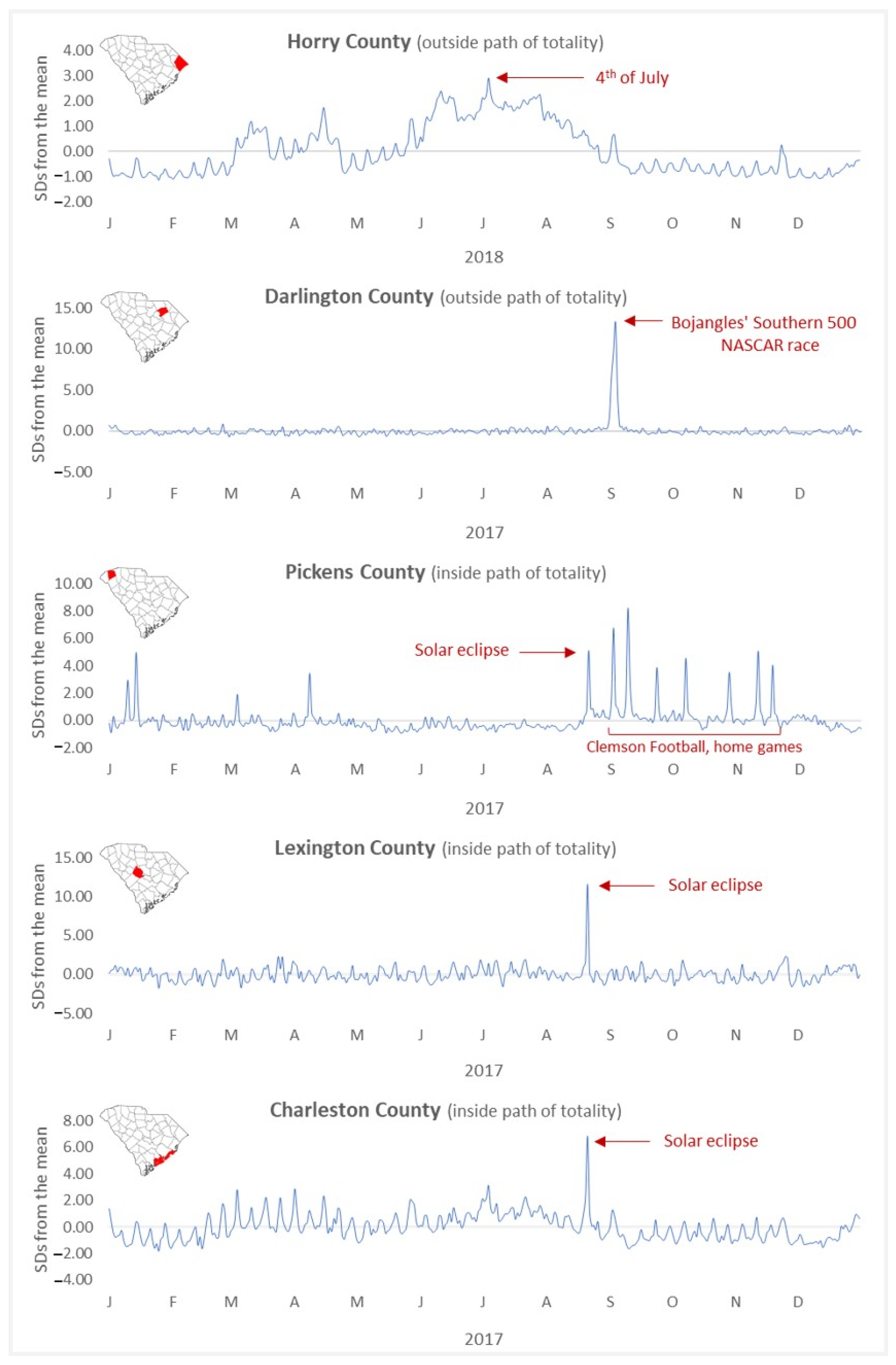
4.3.1. Visitor Dynamics in South Carolina

To facilitate comparison along the year and across the different counties, a nine-interval divergent legend (fewer visitors than the average in brown shades and more visitors than the average in green shades) was designed to represent the daily Twitter non-residents standard score computed with Equation (1).
On 19 August 2017 (Figure 4A), we can identify the first effects of the Solar Eclipse on the influxes of visitors, with several counties with +1 or +1.5 standard deviations from the county’s year non-resident average. On 20 August (Figure 4B), the pattern becomes more obvious, particularly centered in the Columbia metropolitan area (Richland and Lexington counties) and the central coastal counties. On 21 August (Figure 4C), the day of the solar eclipse, most of the state recorded over two standard deviations above the mean in the daily percentages of visitors, indicating that this day was exceptional for most of the counties, especially those in the path of totality. Green shades are still present on 22 August, indicating that many visitors did not leave SC right after the solar eclipse. By 23 August, the low season scenario returns and grey and brown shades are predominant.
We further estimated this normality by averaging the number of visitors of the following days: Monday, 22 August 2016; Monday, 20 August 2018; and Monday, 19 August 2019. We found that SC counties in the totality path registered, on average, around 550% more visitors in comparison with what could be considered normal for the third Monday of August. Counties outside of the totality path registered 180% more visitors than the normal values.
Figure 5 shows the annual distribution of visitors for five counties (two outside the totality path and three inside of this totality path). Horry and Darlington counties, outside of the totality path, do not have a maximum on the day of the eclipse. Horry County shows a low–high season pattern with a maximum on 4 July. Darlington county has a major peak on Labor Day Weekend, coinciding with the annual celebration of the Bojangles’ Southern 500 NASCAR race, which attracts to this small community tens of thousands of visitors during the whole weekend. Pickens County shows an interesting Twitter non-resident distribution across the year. Being in the totality path, we can observe a great influx of visitors around 21 August, but this is not the highest peak of the year. This county, home of the Clemson college football team, has a multipeak distribution coinciding with Clemson home games during the fall. Lexington County, in the central area of SC, does not stand out as a touristy location, but it did experience a major arrival of visitors around the eclipse. In the Charleston graphic, we can easily observe a serrated distribution across the year due to weekday–weekend duality (higher visitation during weekends) and a pronounced peak coinciding with the eclipse.

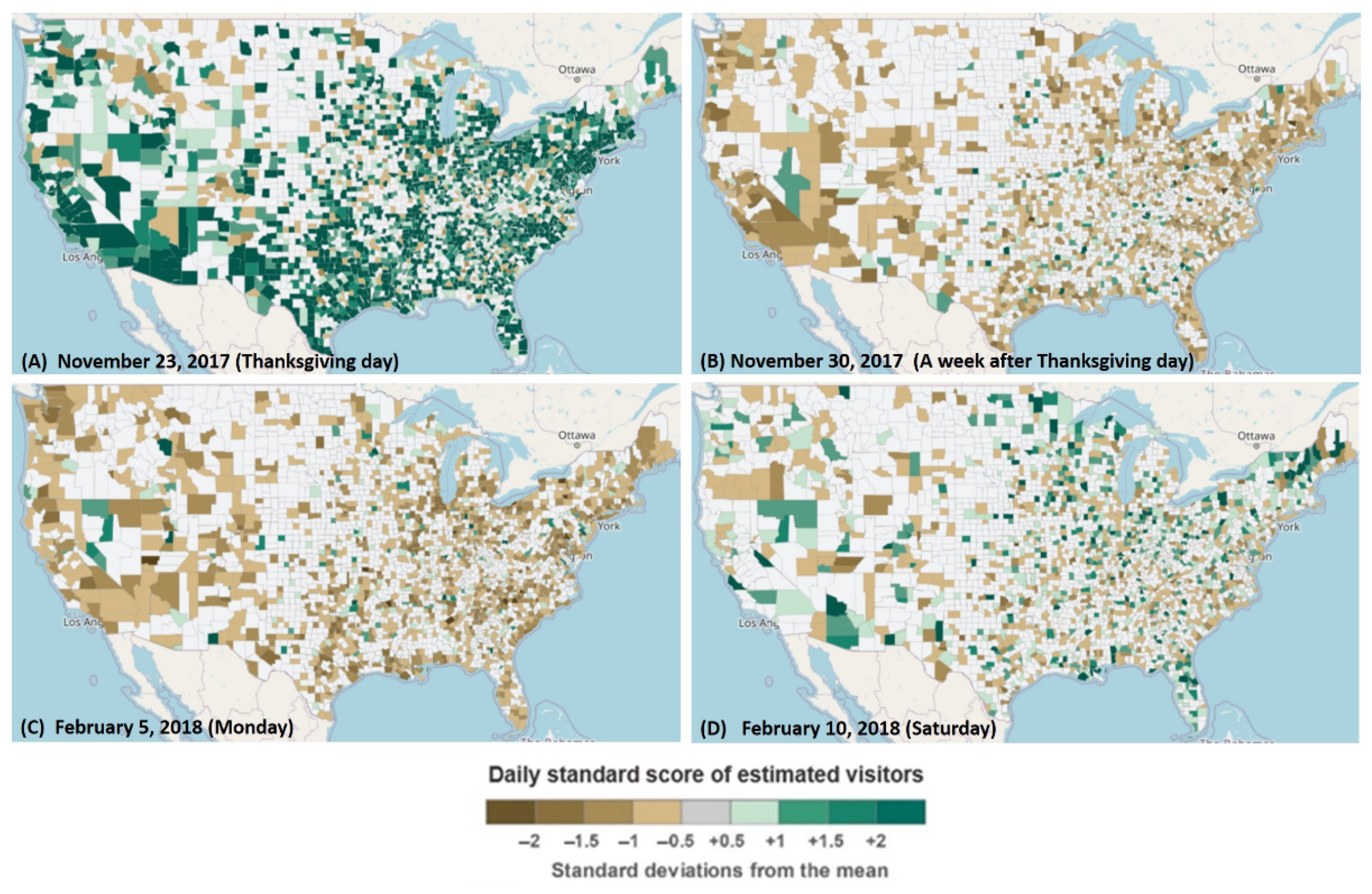
4.3.2. National Scale Analysis

To examine the performance of our approach in revealing the spatiotemporal dynamics of visitors at the national scale, we map the z-score of visitors from 19 August to 23 August 2017 for the contiguous US (Figure 6). The early effects of the Eclipse can be observed on August 19 when the national parks along the totality path (e.g., Yellowstone and Crater Lake) start to attract more visitors than normal. The pattern becomes more obvious on 20 August as the green shades start to emerge along the totality path. On the day of the solar eclipse (21 August), all the counties within the totality path recorded over two standard deviations above the mean in the daily percentages of visitors, resulting in a clear green belt matching well with the totality path. The day after the solar eclipse (22 August), the green belt begins to fade but is still observable, especially around the national parks, indicating that many visitors did not leave after the solar eclipse. On 23 August, the green belt disappears; however, many visitors still did not leave the Yellowstone National Park area.
Following the proposed method, we further computed the county daily z-score of the Twitter non-residents (visitors) for the entire contiguous US for three years including 2017, 2018, and 2019. An interactive web portal1 is developed to interactively visualize the daily spatial patterns and temporal trends for any selected date or county within the time period. Figure 7 shows a snapshot of Twitter non-residents for four selected days in 2017 and 2018 visualized using the portal, revealing clear holiday and weekday–weekend variations in a national scale. Figure 7A reveals the prevalence of travels on Thanksgiving Day (23 November 2017) as most counties in the continuous US recorded over two standard deviations above the mean (green counties) in the daily percentages of visitors. A week after Thanksgiving Day (30 November 2017), grey and brown shades are predominant in the map (Figure 7B), indicating a normal scenario with less travels. Similar patterns are observed during different days of the week. For example, Monday (Figure 7C) shows less visitors while Saturday (Figure 7D) shows more visitors, though the intensity is less dramatic than Thanksgiving Day. A video animation2 has been created to demonstrate the spatial patterns of Twitter visitors for selected dates in 2018, which reveals clear holiday and seasonal variations at a national scale.
The results of this case study demonstrate that the presented approach is operatively valid to estimate the magnitude of non-resident visitations at the county and daily scales. This research not only validates the resident/non-resident classification approach employed but showcases the potential application of the method for near real-time population estimation when combined with other sources of data such as surveys (Alexander et al. 2020).

5. Conclusions and Future Work

This work intends to offer insights towards an automated Twitter census that can provide a more temporally granular picture of the local and non-local populations at the county level. Focusing on data from 2017, we designed a method that precisely determines—success rate around 80% according to internal validation based on self-reported home location—the residential location of a Twitter user based on their tweeting activity. An external validation confirmed that the yearly aggregated results of Twitter residents from our method correlate well with 5-year ACS county population estimates. In addition, the monthly aggregated Twitter non-residents found a strong positive relationship with a tourism indicator such as the monthly state accommodation tax at the county level. Altogether, this external validation helped to confirm the validity of the approach.
The case study of the 2017 US Solar Eclipse further confirmed the potential and validity of the approach as it added intuitive sense to the data resulting from our method. The method was able to estimate the magnitude of the extraordinary influx of Twitter users at the county level, in particular to counties under the path of totality, by comparing it with normal expected visitation levels. The resulting data were also able to identify high/low visitation seasons, weekday/weekend visitation patterns and detect other events, such as college football games or a NASCAR race in SC. It should be noted that our approach did not account for potential increases in tweeting activity during special events. In other words, people might tend to tweet more frequently during particular events such as disasters, which could increase the identified resident and non-resident users in a county. This limitation can be, in part, addressed by using several years of data to offset/normalize this effect using the total daily tweets sent in each county.
Another aspect that must be discussed due to its relevance is the representativeness of Twitter data. The sample we investigated is a subset (only geotagged tweets) of the 1% of the total Twitter content, which is what the company make available through its Application Programming Interface (API) (Burton et al. 2012). Our sample consists of about 80% of tweets tagged at the place level (city, neighborhood, and point of interest) with the remaining tweets geotagged with coordinates (latitude and longitude) (Li et al. 2021b). It must be noted that Twitter data, and therefore, our sample, are just representative of themselves (the Twitter population), which several studies have concluded have urban, gender (male), and race (Caucasian) biases (Mislove et al. 2011; Hecht and Stephens 2014). In addition, these biases of differential usage are not equally distributed across time and space, as Jiang et al. (2018) demonstrated by spatially analyzing the different characteristics of Twitter users. While we are fully aware of this representativeness shortcoming and by no means intend to directly associate our Twitter population estimates (residents/non-residents) with the general population estimates, we believe the inclusion of the dynamic component extracted in this study to models that take into consideration the different biases of Twitter data and potentially incorporate and combine data from other sources can indeed bring us closer to a real daily updated population census. This study must therefore be taken as a necessary step to that ultimate goal and that is why we make our results available through the interactive web portal.
In follow-up projects, we intend to apply the method to other countries of the world and make the information available in near real-time, which would be of great help to follow dynamic processes such as evacuations or shelter-in-place orders during emergencies. We believe this new dataset could benefit various fields such as demography, geography, tourism, emergency management, and public health and create new opportunities for large-scale mobility analyses, as it can introduce the dynamic component often lacking in population estimates. For instance, the creation of worldwide real-time monitoring of the spatial behavior of the population would be particularly relevant during emergencies such as the COVID-19 crisis, where identifying where a population is concentrating in near real-time or determining whether people are complying with shelter-in-place official orders becomes a top priority for authorities. Even though this is just an initial step and more detailed analyses would be needed to blend Twitter with other sources such as surveys and SafeGraph data (https://www.safegraph.com, accessed on 13 June 2021) and model the intrinsic biases associated with social media data, geotagged tweets, as one of the few forms of freely available geospatial digital trace data, hold promise for the understanding of human spatial behavior under normal and extraordinary conditions such as the COVID-19 global crisis.

Author Contributions

Conceptualization, Y.M., Z.L., Y.G.; methodology, Y.M., Z.L.; software, Z.L., X.H.; validation, Y.M. and Z.L.; formal analysis, Y.M., Z.L.; investigation, Y.M., Z.L.; resources, Z.L., Y.G.; data curation, Z.L., X.H.; writing—original draft preparation, Y.M.; writing—review and editing, Z.L., Y.M., Y.G., X.H.; visualization, Y.M., Z.L., X.H.; supervision, Y.G., Z.L.; project administration, Y.G., Z.L.; funding acquisition, Z.L., Y.G. All authors have read and agreed to the published version of the manuscript.

Funding

The research is in part supported by National Science Foundation (2028791) to Z.L.; and University of South Carolina COVID-19 Internal Funding Initiative (135400-20-54176) to Z.L. The first and third authors were supported by the Urban Resilience Initiative at the University of Central Florida. The funders had no role in study design, data collection and analysis, decision to publish, or preparation of the manuscript.

Data Availability Statement

Geotagged tweets were collected using Twitter’s public Streaming API from the public domain following Twitter’s Developer Agreement. Following Twitter’s policy on “Redistribution of Twitter content” (https://developer.twitter.com/en/developerterms/more-on-restricted-use-cases, accessed on 13 June 2021), the geotagged tweet IDs used in this analysis can be shared upon request.

Conflicts of Interest

The authors declare no conflict of interest.

Note

1
2

References

  1. Alexander, Monica, Emilio Zagheni, and Kivan Polimis. 2019. The impact of Hurricane Maria on out-migration from Puerto Rico: Evidence from Facebook data. SocArXiv. [Google Scholar] [CrossRef] [Green Version]
  2. Alexander, Monica, Kivan Polimis, and Emilio Zagheni. 2020. Combining social media and survey data to nowcast migrant stocks in the United States. Population Research and Policy Review. [Google Scholar] [CrossRef]
  3. Amini, Alexander, Kevin Kung, Chaogui Kang, Stanislav Sobolevsky, and Carlo Ratti. 2014. The impact of social segregation on human mobility in developing and industrialized regions. EPJ Data Science 3: 1–20. [Google Scholar] [CrossRef] [Green Version]
  4. Barslund, Mikkel, and Matthias Busse. 2016. How Mobile Is Tech Talent? A Case Study of IT Professionals Based on Data from LinkedIn (CEPS Special Report, No. 140). Available online: https://ssrn.com/abstract=2859399 (accessed on 13 June 2021).
  5. Bell, Martin, Elin Charles-Edwards, Dorota Kupiszewska, Marek Kupiszewski, John Stillwell, and Yu Zhu. 2015. Internal migration data around the world: Assessing contemporary practice. Population, Space and Place 21: 1–17. [Google Scholar] [CrossRef]
  6. Bengtsson, Linus, Xin Lu, Anna Thorson, Richard Garfield, and Johan von Schreeb. 2011. Improved response to disasters and outbreaks by tracking population movements with mobile phone network data: A post-earthquake geospatial study in Haiti. PLoS Medicine 8: e1001083. [Google Scholar] [CrossRef]
  7. Billari, Francesco C., and Emilio Zagheni. 2017. Big Data and Population Processes: A Revolution? SocArXiv. [Google Scholar] [CrossRef]
  8. Bisanzio, Donal, Moritz U. Kraemer, Isaac I. Bogoch, Thomas Brewer, John S. Brownstein, and Richard Reithinger. 2020. Use of Twitter social media activity as a proxy for human mobility to predict the spatiotemporal spread of COVID-19 at global scale. Geospatial Health 15. [Google Scholar] [CrossRef]
  9. Bittermann, André, Veronika Batzdorfer, Sarah Marie Müller, and Holger Steinmetz. 2021. Mining Twitter to Detect Hotspots in Psychology. Zeitschrift für Psychologie 229: 3–14. [Google Scholar] [CrossRef]
  10. Blumenstock, Joshua. E. 2012. Inferring patterns of internal migration from mobile phone call records: Evidence from Rwanda. Information Technology for Development 18: 107–25. [Google Scholar] [CrossRef]
  11. Boyle, Rebecca. 2017. The Largest Mass Migration to See a Natural Event Is Coming. The Atlantic. Available online: https://www.theatlantic.com/science/archive/2017/08/the-greatest-mass-migration-in-american-history/535734/ (accessed on 13 June 2021).
  12. Burton, Scott H., Kesler W. Tanner, Christophe G. Giraud-Carrier, Joshua H. West, and Michael D. Barnes. 2012. “Right time, right place” health communication on Twitter: Value and accuracy of location information. Journal of Medical Internet Research 14. [Google Scholar] [CrossRef]
  13. Cesare, Nina, Hedwig Lee, Tyler McCormick, Emma Spiro, and Emilio Zagheni. 2018. Promises and pitfalls of using digital traces for demographic research. Demography 55: 1979–99. [Google Scholar] [CrossRef]
  14. Coleman, David. 2013. The twillight of the census. Population and Development Review 38: 334–51. [Google Scholar] [CrossRef]
  15. Colleoni, Matteo. 2016. A social science approach to the study of mobility: An introduction. In Understanding Mobilities for Designing Contemporary Cities. Edited by Paola Pucci and Matteo Colleoni. Cham: Springer, pp. 23–33. [Google Scholar] [CrossRef]
  16. Cresswell, Tim. 2011. Mobilities I: Catching up. Progress in Human Geography 35: 550–58. [Google Scholar] [CrossRef]
  17. Ćurlin, Tamara, Božidar Jaković, and Ivan Miloloža. 2019. Twitter usage in tourism: Literature review. Business Systems Research: International Journal of the Society for Advancing Innovation and Research in Economy 10: 102–19. [Google Scholar] [CrossRef] [Green Version]
  18. Ester, Martin, Hans-Peter Kriegel, Jörg Sander, and Xiaowei Xu. 1996. A density-based algorithm for discovering clusters in large spatial databases with noise. Kdd 96: 226–31. [Google Scholar]
  19. Faggian, Alessandra, and Philip McCann. 2008. Human capital, graduate migration and innovation in British regions. Cambridge Journal of Economics 33: 317–33. [Google Scholar] [CrossRef] [Green Version]
  20. Franklin, Rachel S., and David A. Plane. 2006. Pandora’s box: The potential and peril of migration data from the American Community Survey. International Regional Science Review 29: 231–46. [Google Scholar] [CrossRef]
  21. Fussell, Elizabeth, Lori M. Hunter, and Clark L. Gray. 2014. Measuring the environmental dimensions of human migration: The demographer’s toolkit. Global Environmental Change 28: 182–91. [Google Scholar] [CrossRef] [Green Version]
  22. Fussell, Elizabeth, Sara R. Curran, Matthew D. Dunbar, Michael A. Babb, Luanne Thompson, and Jacqueline Meijer-Irons. 2017. Weather-related hazards and population change: A study of hurricanes and tropical storms in the United States, 1980–2012. The Annals of the American Academy of Political and Social Science 669: 146–67. [Google Scholar] [CrossRef] [PubMed]
  23. Harvey, David. 1989. The Condition of Postmodernity. An Enquiry into the Origins of Cultural Change. Oxford: Blackwell. [Google Scholar]
  24. Hawelka, Bartosz, Isabela Sitko, Euro Beinat, Stanislav Sobolevsky, Pavlos Kazakopoulos, and Carlo Ratti. 2014. Geo-located Twitter as proxy for global mobility patterns. Cartography and Geographic Information Science 41: 260–71. [Google Scholar] [CrossRef] [Green Version]
  25. Hecht, Brent J., and Monica Stephens. 2014. A tale of cities: Urban biases in volunteered geographic information. ICWSM 14: 197–205. [Google Scholar]
  26. Hu, Fei, Zhenlong Li, Chaowei Yang, and Yongyao Jiang. 2019. A graph-based approach to detecting tourist movement patterns using social media data. Cartography and Geographic Information Science 46: 368–82. [Google Scholar] [CrossRef]
  27. Huang, Qunying, and Yu Xiao. 2015. Geographic situational awareness: Mining tweets for disaster preparedness, emergency response, impact, and recovery. ISPRS International Journal of Geo-Information 4: 1549–68. [Google Scholar] [CrossRef] [Green Version]
  28. Huang, Xiao, Cuizhen Wang, and Zhenlong Li. 2018. Reconstructing flood inundation probability by enhancing near real-time imagery with real-time gauges and tweets. IEEE Transactions on Geoscience and Remote Sensing 56: 4691–701. [Google Scholar] [CrossRef]
  29. Huang, Xiao, Zhenlong Li, Cuizhen Wang, and Huan Ning. 2019. Identifying disaster related social media for rapid response: A visual-textual fused CNN architecture. International Journal of Digital Earth 13: 1017–39. [Google Scholar] [CrossRef]
  30. Huang, Xiao, Zhenlong Li, Yuqin Jiang, Xiaoming Li, and Dwayne Porter. 2020. Twitter reveals human mobility dynamics during the COVID-19 pandemic. PLoS ONE 15: e0241957. [Google Scholar] [CrossRef] [PubMed]
  31. Isaacson, Michal, and Noam Shoval. 2006. Application of tracking technologies to the study of pedestrian spatial behavior. The Professional Geographer 58: 172–83. [Google Scholar] [CrossRef]
  32. Jiang, Yuqin, Zhenlong Li, and Susan L. Cutter. 2019. Social Network, Activity Space, Sentiment, and Evacuation: What Can Social Media Tell Us? Annals of the American Association of Geographers 109: 1795–810. [Google Scholar] [CrossRef]
  33. Jiang, Yuqin, Zhenlong Li, and Xinyue Ye. 2018. Understanding demographic and socioeconomic biases of geotagged Twitter users at the county level. Cartography and Geographic Information Science 46: 228–42. [Google Scholar] [CrossRef]
  34. Jurdak, Raja, Kun Zhao, Jiajun Liu, Maurice AbouJaoude, Mark Cameron, and David Newth. 2015. Understanding human mobility from Twitter. PLoS ONE 10: e0131469. [Google Scholar] [CrossRef] [PubMed]
  35. Kikas, Riivo, Marlon Dumas, and Ando Saabas. 2015. Explaining international migration in the skype network: The role of social network features. Paper presented at 1st ACM Workshop on Social Media World Sensors, Guzelyurt, Cyprus, September 17–22; pp. 17–22. [Google Scholar] [CrossRef]
  36. Koylu, Caglar. 2018. Discovering multi-scale community structures from the interpersonal communication network on Twitter. In Agent-Based Models and Complexity Science in the Age of Geospatial Big Data. Cham: Springer, pp. 87–102. [Google Scholar]
  37. Laczko, Frank. 2015. Factoring migration into the development data revolution. Journal of International Affairs 68: 1. [Google Scholar]
  38. Li, Zhenlong, Cuizhen Wang, Christopher T. Emrich, and Diansheng Guo. 2018. A novel approach to leveraging social media for rapid flood mapping: A case study of the 2015 South Carolina floods. Cartography and Geographic Information Science 45: 97–110. [Google Scholar] [CrossRef]
  39. Li, Zhenlong, Shan Qiao, Yuqin Jiang, and Xiaoming Li. 2021a. Building a Social media-based HIV Risk Behavior Index to Inform the Prediction of HIV New Diagnosis: A Feasibility Study. AIDS 35: S91–S99. [Google Scholar] [CrossRef]
  40. Li, Zhenlong, Xiao Huang, Xinyue Ye, Yuqin Jiang, Martín Yago, Huan Ning, Michael E. Hodgson, and Xiaoming Li. 2021b. Measuring Global Multi-Scale Place Connectivity using Geotagged Social Media Data. arXiv arXiv:2102.03991. [Google Scholar]
  41. Li, Zhenlong, Xiao Huang, Tao Hu, Huan Ning, Xinyue Ye, and Xiaoming Li. 2021C. ODT FLOW: A Scalable Platform for Extracting, Analyzing, and Sharing Multi-source Multi-scale Human Mobility. arXiv arXiv:2104.05040. [Google Scholar]
  42. Lin, Jie, and Robert G. Cromley. 2018. Inferring the home locations of Twitter users based on the spatiotemporal clustering of Twitter data. Transactions in GIS 22: 82–97. [Google Scholar] [CrossRef]
  43. Mallick, Bishawjit, and Joachim Vogt. 2014. Population displacement after cyclone and its consequences: Empirical evidence from coastal Bangladesh. Natural Hazards 73: 191–212. [Google Scholar] [CrossRef]
  44. Martín, Yago, Susan L. Cutter, and Zhenlong Li. 2020a. Bridging twitter and survey data for evacuation assessment of Hurricane Matthew and Hurricane Irma. Natural Hazards Review 21: 04020003. [Google Scholar] [CrossRef]
  45. Martín, Yago, Susan L. Cutter, Zhenlong Li, Christopher T. Emrich, and Jerry T. Mitchell. 2020b. Using geotagged tweets to track population movements to and from Puerto Rico after Hurricane Maria. Population and Environment 42: 4–27. [Google Scholar] [CrossRef]
  46. Martín, Yago, Zhenlong Li, and Susan L. Cutter. 2017. Leveraging Twitter to gauge evacuation compliance: Spatiotemporal analysis of Hurricane Matthew. PLoS ONE 12: e0181701. [Google Scholar] [CrossRef] [PubMed] [Green Version]
  47. McNeill, Graham, Jonathan Bright, and Scott A. Hale. 2017. Estimating local commuting patterns from geolocated Twitter data. EPJ Data Science 6: 24. [Google Scholar] [CrossRef] [Green Version]
  48. Messias, Johnnatan, Fabrício Benevenuto, Ingmar Weber, and Emilio Zagheni. 2016. From migration corridors to clusters: The value of Google+ data for migration studies. Paper presented at 2016 IEEE/ACM International Conference on Advances in Social Networks Analysis and Mining, San Francisco, CA, USA, August 18–21; pp. 421–28. [Google Scholar] [CrossRef] [Green Version]
  49. Mislove, Alan, Sune Lehmann, Yong-Yeol Ahn, Jukka-Pekka Onnela, and James N. Rosenquist. 2011. Understanding the demographics of Twitter users. Paper presented at Fifth International AAAI Conference on Weblogs and Social Media, Barcelona, Spain, July 17–21; Available online: http://www.aaai.org/ocs/index.php/ICWSM/ICWSM11/paper/viewFile/2816/3234 (accessed on 13 June 2021).
  50. Pershad, Yash, Patrick T. Hangge, Hassan Albadawi, and Rahmi Oklu. 2018. Social medicine: Twitter in healthcare. Journal of Clinical Medicine 7: 121. [Google Scholar] [CrossRef] [Green Version]
  51. Rango, Marzia, and Michele Vespe. 2017. Big Data and Alternative Data Sources on Migration: From Case-Studies to Policy Support (Summary report European Commission—Joint Research Centre). Available online: https://gmdac.iom.int/big-data-and-alternative-data-sources-on-migration-from-case-studies-to-policy-support (accessed on 13 June 2021).
  52. Roberts, Helen, Jon Sadler, and Lee Chapman. 2019. The value of Twitter data for determining the emotional responses of people to urban green spaces: A case study and critical evaluation. Urban Studies 56: 818–35. [Google Scholar] [CrossRef]
  53. SCPRT—South Carolina Department of Parks, Recreation and Tourism. 2019. Research and Statistics. Available online: https://www.scprt.com/research (accessed on 13 June 2021).
  54. Sheffer, Mary L., and Brad Schultz. 2010. Paradigm shift or passing fad? Twitter and sports journalism. International Journal of Sport Communication 3: 472–84. [Google Scholar] [CrossRef]
  55. Skeldon, Ronald. 2012. Migration and its measurement: Towards a more robust map of bilateral flows. In Handbook of Research Methods in Migration. Edited by Carlos Vargas-Silva. Cheltenham: Edward Elgar Publishing Ltd., pp. 229–48. [Google Scholar]
  56. Spyratos, Spyridon, Michele Vespe, Fabrizio Natale, Ingmar Weber, Emilio Zagheni, and M. Rango. 2018. Migration Data Using Social Media: A EUROPEAN Perspective (EUR 29273 EN). Luxembourg: Publications Office of the European Union. [Google Scholar] [CrossRef]
  57. Squire, Vicki, ed. 2010. The Contested Politics of Mobility: Borderzones and Irregularity. New York: Routledge. [Google Scholar]
  58. Stock, Kristin. 2018. Mining location from social media: A systematic review. Computers, Environment and Urban Systems 71: 209–40. [Google Scholar] [CrossRef]
  59. Takhteyev, Yuri, Anatoliy Gruzd, and Barry Wellman. 2012. Geography of Twitter networks. Social Networks 34: 73–81. [Google Scholar] [CrossRef]
  60. Tamgno, James. K., Roger M. Faye, and Claude Lishou. 2013. Verbal autopsies, mobile data collection for monitoring and warning causes of deaths. Paper presented at 2013 15th International Conference on Advanced Communications Technology (ICACT), PyeongChang, Korea, January 27–30; pp. 495–501. [Google Scholar]
  61. Taylor, Linnet. 2016. No place to hide? The ethics and analytics of tracking mobility using mobile phone data. Environment and Planning D: Society and Space 34: 319–36. [Google Scholar] [CrossRef]
  62. Tinati, Ramine, Susan Halford, Leslie Carr, and Catherine Pope. 2014. Big data: Methodological challenges and approaches for sociological analysis. Sociology 48: 663–81. [Google Scholar] [CrossRef] [Green Version]
  63. Traunmueller, Martin W., Nicholas Johnson, Awais Malik, and Constantine E. Kontokosta. 2018. Digital footprints: Using WiFi probe and locational data to analyze human mobility trajectories in cities. Computers, Environment and Urban Systems 72: 4–12. [Google Scholar] [CrossRef]
  64. Turner, Ash. 2020. How Many Smartphones Are in the World? Available online: https://www.bankmycell.com/blog/how-many-phones-are-in-the-world (accessed on 13 June 2021).
  65. United Nations. 2008. Principles and Recommendations for Population and Housing Censuses (Statistical Papers (Seri. M)). New York: United Nations. [Google Scholar] [CrossRef]
  66. Wesolowski, Amy, Caroline O. Buckee, Linus Bengtsson, Erik Wetter, Xin Lu, and Andrew J. Tatem. 2014. Commentary: Containing the Ebola outbreak-the potential and challenge of mobile network data. PLoS Currents, 6. [Google Scholar] [CrossRef] [PubMed]
  67. Wesolowski, Amy, Nathan Eagle, Andrew J. Tatem, David L. Smith, Abdisalan M. Noor, Robert W. Snow, and Caroline O. Buckee. 2012. Quantifying the impact of human mobility on malaria. Science 338: 267–70. [Google Scholar] [CrossRef] [PubMed] [Green Version]
  68. Willekens, Frans, Douglas Massey, James Raymer, and Cris Beauchemin. 2016. International migration under the microscope. Science 352: 897–99. [Google Scholar] [CrossRef] [Green Version]
  69. Zagheni, Emilio, and Ingmar Weber. 2012. You are where you e-mail: Using e-mail data to estimate international migration rates. Paper presented at 4th Annual ACM Web Science Conference, Evanston, IL, USA, June 22–24; pp. 348–51. [Google Scholar] [CrossRef]
  70. Zagheni, Emilio, Ingmar Weber, and Krishna Gummadi. 2017. Leveraging Facebook’s advertising platform to monitor stocks of migrants. Population and Development Review 43: 721–34. [Google Scholar] [CrossRef]
  71. Zagheni, Emilio, Kivan Polimis, Monica Alexander, Ingmar Weber, and Francesco C. Billari. 2018. Combining social media data and traditional surveys to nowcast migration stocks. Paper presented at Annual Meeting of the Population Association of America, Austin, TX, USA, April 10–13. [Google Scholar]
  72. Zagheni, Emilio, Venkata R. K. Garimella, and Ingmar Weber. 2014. Inferring international and internal migration patterns from twitter data. Paper presented at 23rd International Conference on World Wide Web, Seoul, Korea, April 7–11; pp. 439–44. [Google Scholar] [CrossRef]
  73. Zeiler, Michael. 2017. Predicting Eclipse Visitation with Population Statistics. Available online: https://www.greatamericaneclipse.com/statistics/ (accessed on 13 June 2021).
Figure 1. Path of the 2017 Solar Eclipse totality in South Carolina and across the US.
Socsci 10 00227 g001
Figure 2. Scatter plot of 5-year ACS county population estimates and the daily average of total active Twitter residents per county (46 counties in SC).
Socsci 10 00227 g002
Figure 3. (A) Log-log plots of the relationship between monthly accommodation tax per county and the average of monthly non-resident Twitter users per county. (B) R2 values of this relationship across year 2017.
Socsci 10 00227 g003
Figure 4. Daily standard score of estimated visitors from 19 August to 22 August 2017 in South Carolina. (A) Saturday, 19 August 2017, (B) Saturday, 20 August 2017, (C) Saturday, 21 August 2017 (solar eclipse day), (D) Saturday, 22 August 2017.
Socsci 10 00227 g004
Figure 5. Annual distribution of Twitter non-residents (expressed in daily standard deviations from the mean) for five SC counties: outside of the path of totality (Horry County and Darlington County) and inside of the path of totality (Pickens County, Lexington County, and Charleston County).
Socsci 10 00227 g005
Figure 6. Daily standard score of estimated visitors from 19 August to 23 August 2017 for the contiguous US.
Socsci 10 00227 g006
Figure 7. A snapshot of standard score of estimated visitors for four selected days in 2017 and 2018 visualized using the portal, revealing clear holiday and weekday–weekend patterns in a national scale. (A) 23 November 2017 (Thanksgiving Day), (B) 30 November 2017 (A week after the Thanksgiving Day), (C) 5 February 2018 (Monday), (D) 10 February 2018 (Saturday).
Socsci 10 00227 g007
Table 1. Percentages of successful home location identification for different thresholds.
Users% Total% Successful
Cannot compute mode284.24%/
All users *633100.0%77.3%
Users 3 tweets or more *63199.7%77.3%
Users 5 tweets or more *61697.3%77.6%
Users 10 tweets or more *58291.9%77.8%
Users 15 tweets or more *54786.4%77.1%
Users 20 tweets or more *51581.4%77.7%
Users 25 tweets or more *48376.3%78.1%
Users 30 tweets or more *46673.6%78.1%
Users 50 tweets or more *38761.1%78.3%
Users 100 tweets or more *27443.3%78.5%
Users 200 tweets or more *16626.2%82.5%
Users 500 tweets or more *589.2%82.8%
Users 1000 tweets or more *182.8%83.3%
* After removing those whose mode could not be computed.
Table 2. Issues identified during the analysis of home location misidentifications.
Affected CountiesUsers% Total
Fulton (GA)/Gwinnett (GA)10.7%
Charleston/Dorchester/Berkeley117.6%
Richland/Lexington1510.4%
Pickens/Greenville53.5%
York/Lancaster53.5%
Publisher’s Note: MDPI stays neutral with regard to jurisdictional claims in published maps and institutional affiliations.

