Prediction of the Maximum Seismic Member Force in a Superstructure of a Base-Isolated Frame Building by Using Pushover Analysis


Department of Architecture, Faculty of Creative Engineering, Chiba Institute of Technology, Chiba 275-0016, Japan
Buildings 2019, 9(9), 201; https://doi.org/10.3390/buildings9090201
Submission received: 13 August 2019
/
Revised: 29 August 2019
/
Accepted: 3 September 2019
/
Published: 5 September 2019
(This article belongs to the Special Issue Smart Solutions and Structural Systems for Seismic-Resistant Buildings)
Abstract
:It is essential for the seismic design of a base-isolated building that the seismic response of the superstructure remains within the elastic range. The evaluation of the maximum seismic member force in a superstructure is thus an important issue. The present study predicts the maximum seismic member force of five- and fourteen-story reinforced concrete base-isolated frame buildings adopting pushover analysis. In the first stage of the study, the nonlinear dynamic (time-history) analysis of the base-isolated frame buildings is carried out, and the nonlinear modal responses of the first and second modes are calculated from pushover analysis results. In the second stage, a set of pushover analyses is proposed considering the combination of the first and second modal responses, and predicted maximum member forces are compared with the nonlinear time-history analysis results. Results show that the maximum member forces predicted in the proposed set of pushover analyses are satisfactorily accurate, while the results predicted considering only the first mode are inaccurate.
1. Introduction
Seismic isolation is widely applied to buildings for earthquake protection in earthquake-prone countries [1]. Unlike the case for traditional earthquake-resistant structures, seismic isolation ensures the behaviors of building structures are within the elastic range and the reduction of the acceleration in the buildings during a large earthquake. In the case of large seismic excitation, most seismic energy input to the base-isolated building will be absorbed in the isolation layer, and the energy absorbed by the supported superstructure will be limited. In contrast, most seismic energy input to a traditional earthquake-resistant structure will be absorbed as damage to columns and beams, and most traditional earthquake-resistant structures are thus at risk of being demolished in a severe seismic event. It is therefore recommended that the behavior of the supported superstructure of the base-isolated building be elastic in design guidelines for seismically isolated buildings [2]. For the design of the superstructure for base-isolated buildings, some formulas for the vertical distribution of lateral seismic forces have been proposed [3,4]. Lee et al. have proposed a formula based on the combination of the fundamental mode of the base-isolated structure idealized as a two-degree-of-freedom (two-DOF) model and the fundamental mode of a fix-based structure [3]. Although their formula successfully estimates the seismic story shear force of five-story base-isolated building models, it fails to estimate that of fifteen-story base-isolated building models, because the higher mode effect is significant in the distribution of seismic forces in case of taller base-isolated buildings. In addition, their formula cannot consider the nonlinearity of an isolated layer. York and Ryan have proposed a formula considering the nonlinearity of the isolation layer [4]. Their formula is based on a huge number of numerical analysis results and is implemented to the American Society of Civil Engineering (ASCE) standard for seismic retrofit of existing buildings [5]. Although the original purpose of the proposed formula is to determine the design member forces in a superstructure by the linear static analysis, the ASCE standard [5] allows us to use this formula for the nonlinear static analysis, unless some conditions are satisfied, including that the superstructure is less than or equal to four stories or 65 ft in height from the base level.
There have been studies on the nonlinear seismic response of base-isolated buildings considering the nonlinear behavior of superstructures [6,7,8,9]. For example, Kikuchi et al. investigated the inelastic response of base-isolated buildings on the basis of the theoretical solution of the response of a yielding two-DOF model subjected to sinusoidal excitation [7]. They found that the behavior of yielding isolated structures is fundamentally different from that of fixed-base structures, i.e., positive aspects of yielding (i.e., a change in effective frequency and an increase in energy absorption) should not be expected in the case of yielding isolated structures.
In the seismic design of traditional earthquake-resistant structures, a simplified nonlinear analysis procedure, which combines the nonlinear static (pushover) analysis of a multi-degrees-of-freedom model with the response spectrum analysis of an equivalent single-degree-of-freedom (SDOF) model, is available, e.g., the N2 method [10,11] and modal pushover analysis [12]. Although a rigorous nonlinear time-history analysis is required in most cases of the seismic design of seismically isolated buildings, there have been studies on the application of such nonlinear static analysis to base-isolated buildings by Kilar and Koren [13,14,15,16], Providakis [17], Faal and Poursha [18], and Bhandari et al. [19,20]. In most of these investigations, the nonlinearity of the superstructure was considered, and discussions focused on the accuracy of story drift and plastic hinge rotations in comparison with nonlinear time-history analysis results. However, the author understands that there have been no studies on the demand of the member force in the superstructure of a base-isolated building.
As mentioned above, it is essential in the seismic design of a base-isolated building that the seismic response of the superstructure remains within the elastic range. The evaluation of the maximum seismic member force in a superstructure is thus an important issue. Although there are several studies regarding the seismic story shear force of superstructures in base-isolated buildings (e.g., [3,4]), their discussions are mainly focused on the vertical distribution of lateral force applying to the linear static analysis. In case the behavior of the isolated layer is nonlinear, the member force in the superstructure is influenced by the nonlinearity of the isolated layer, even though the superstructure remains elastic. Therefore, the author thinks the better method to calculate the member force in the superstructure is carried out in the nonlinear static analysis of the whole structure, including the nonlinear isolated layer. Of course, the most rigorous method for this purpose is the nonlinear dynamic (time-history) analysis of the whole structure. However, from the author’s point of view, such analysis demands highly engineering judgement, such as detailed modelling of the structural behavior (including the cyclic behavior) and selection of the ground motions and computation costs. Besides, it is very difficult to interpret the analysis results properly: how to understand the fundamental behavior of the analyzed structure is a very tough task for the analysts and also the designers, and the analysis results are highly dependent on the ground motion characteristics. The nonlinear static analysis, in contrast, provides us the basic information about the building under investigation. From this aspect, the author believes the nonlinear static analysis assists designers and analysts in the understanding of the nonlinear behavior of buildings.
The present study predicts the maximum seismic member force of five- and fourteen-story reinforced concrete base-isolated frame buildings adopting pushover analysis. For the simplicity of discussion, the behavior of members in the superstructure is assumed to be linear elastic. The isolated layer of each of the two buildings comprises natural rubber bearings (NRBs), lead-rubber bearings (LRBs), and steel dampers.
The rest of the paper is organized as follows. Section 2 provides basic information on the two model buildings and ground motions. Section 3 carries out the nonlinear time-history analysis of the base-isolated frame buildings and calculates the nonlinear modal responses of the first and second modes using pushover analysis results. Section 4 proposes a set of pushover analyses considering the combination of the first and second modal responses and compares the predicted maximum member forces with the nonlinear time-history analysis results. Discussions are then presented on the accuracy of the proposed pushover analysis for the prediction of the maximum member force of superstructures.
2. Building and Ground Motion Data
2.1. Building Data
The present study investigates the two base-isolated building models shown in Figure 1 and Figure 2. Both models were based on the buildings originally designed as traditional earthquake-resistant structures according to the current seismic design code of Japan and a design example published by Japan Building Disaster Prevention Association (JABDA) [21]. Model-05, shown in Figure 1, is a five-story base-isolated reinforced concrete building model while Model-14, shown in Figure 2, is a 14-story reinforced concrete building model. The weight of floor per unit area above level Z1 and at level Z0 are respectively assumed to be 14 and 32 kN/m2. The member sections, compressive strength, and Young’s modules of concrete for each model are given in Table 1 and Table 2. All beams and columns are assumed to have linear elastic behavior.
The isolated layer below level Z0 comprises NRBs, LRBs, and steel dampers. Figure 3 shows envelopes of the force–deformation relationship for the isolators and damper. The behavior of an NRB is assumed to be linear elastic while that of an LRB and that of a steel damper are assumed to be bilinear.
To determine the properties of the isolated layer, the seismic isolation period, Tf, defined as:
is adjusted between 4.0 to 5.0 seconds. In Equation (1), M is the total mass of the superstructure above the isolated layer and Kf is the total stiffness of the isolated layer without dampers. The shear force coefficient of dampers, αs, is defined by:
In Equation (2), g is the acceleration due to gravity and is assumed to be 9.8 m/s2, sQy is the sum of the yield strength of dampers (including LRBs), Qyd. In this study, αs is adjusted around 0.05.
All isolators are chosen from a catalog provided by Bridgestone Corporation [22], considering the range of nominal stress of each isolator due to a vertical load ranging from 5 to 15 MPa. Meanwhile, the steel dampers used in Model-14 are chosen from a catalog provided by Nippon Steel Corporation Engineering Co. Ltd. [23]. Table 3, Table 4 and Table 5 give the properties of isolators and dampers for the two models.
The isolated period Tf, calculated using K1 of NRBs and K2 of LRBs, is 4.04 s for Model-05 and 4.84 s for Model-14. The shear force coefficient of dampers αs, calculated using QyD of LRBs and steel dampers, is 0.055 for Model-05 and 0.048 for Model-14.
The two buildings are modelled as three-dimensional spatial frames, wherein the floor diaphragms are assumed to be rigid in their own planes without out-of-plane stiffness. For numerical analyses, the nonlinear analysis program for spatial frames developed by the author in a previous study [24] is upgraded for the base-isolated buildings. The beams are modelled as an elastic line element with a rigid zone at each end and a length assumed as half the depth of the intersected column minus one-fourth the depth of the considered beam. Similarly, the columns are modelled as an elastic line element with a rigid zone at each end and a length assumed as half the depth of the intersected beam minus one-fourth the depth of the considered column. The shear behavior of isolators is modelled using the multiple-shear-spring model proposed by Wada and Hirose [25]. The vertical behavior of isolators is assumed to be linear elastic while the bending stiffness of isolators is ignored. The steel dampers installed in Model-14 are modelled as two orthogonal shear springs. The hysteresis behavior of LRBs and steel dampers is modelled as following the normal bilinear rule for simplicity of analysis. In determining the damping of the superstructure, eigenvalue analysis is carried out to obtain the natural period of the first mode, assuming the superstructure is pin supported. The damping matrix of the superstructure is then assumed to be proportional to the stiffness matrix of the superstructure, with 2% of the first mode’s critical damping. The damping of isolators and dampers is not considered, assuming their energy absorption effects are already included in the hysteresis rule.
Figure 4 shows the first two natural modes of the two building models in the elastic stage, considering the initial stiffness of LRBs and steel dampers. Note that only natural modes in the X-direction are shown here because the present study considers unidirectional excitation in the X-direction and the two buildings are symmetric across the X- and Y-axes. Here, Tie is the ith natural period in the elastic range (i = 1, 2) and mie* is the equivalent (effective) modal mass ratio of the ith mode.
As shown in Figure 4, the equivalent first modal mass ratio is close to 1 for both models. Therefore, the buildings may oscillate predominantly in the first mode.
2.2. Ground Motion Data
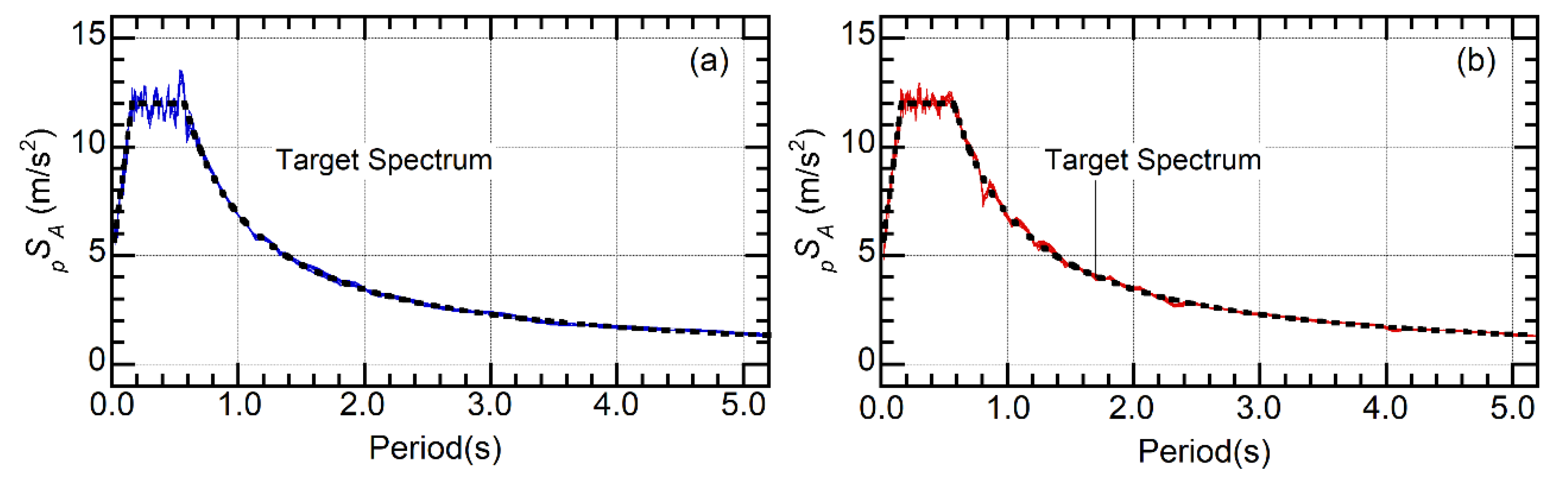
Two series of artificial ground motions are used for the nonlinear time-history analysis. The target elastic spectrum with 5% critical damping, pSA(T, 0.05), is determined from the Building Standard Law of Japan considering the type-1 (rock) soil condition. Two records are used to determine the phase angle of artificial ground motions. One is the horizontal major component of the 1995 Japan Meteorological Agency (JMA) Kobe record while the other is the horizontal major component of Sendai Government Office building #2 recorded during the 2011 earthquake that struck off the Pacific coast of Tohoku [26] (respectively referred to as the JKB record and SND record). The scheme of the generation of artificial ground motion is the same as that in a previous study [27], except that the range of the natural period considered in spectrum fitting is 0.02 to 10.0 s, as recommended in design guidelines of seismically isolated buildings [2]. The phase angle is shifted by the constant Δϕ0 to generate artificial ground motion with the same phase difference but a different time history. Twelve artificial ground motions are generated for each record by varying Δϕ0 in intervals of π/12 from 0 to 11π12. The Art-S series (wave Art-S00 to Art-S11) are the artificial waves generated from the JKB record while the Art-L series (wave Art-L00 to Art-L11) are the artificial waves generated from the SND record. Figure 5 shows the pseudo acceleration spectra of the generated artificial ground motions while Figure 6 shows an example wave of generated artificial ground motions.
Figure 7 compares the 12 waves of the Art-S series. As far as the whole waveform, from 0 to 30 s, as shown in Figure 7a, is concerned, differences among the 12 waves are not significant, however, differences within a short time are noticeable among the 12 waves, as shown in Figure 7b. These differences are due to the shift in phase angle. In the linear seismic response, it is expected that such a detailed difference in the input acceleration would not notably affect the peak response, however, in the nonlinear seismic response, there may be a notable difference in the peak response, as was found in a previous study [27].
2.3. Cases of Nonlinear Time-history Analysis
In this study, the seismic excitation is considered unidirectional in the X-direction. Nonlinear time-history analyses were carried out using the 2 × 12 = 24 artificial ground motions presented in Section 2.2. The intensity of ground motion was scaled as 50%, 75%, and 100%. Therefore, 3 × 2 × 12 = 72 analyses were carried out for each model.
3. Nonlinear Modal Response
This section carries out nonlinear time-history analyses of the base-isolated frame buildings and then calculates the nonlinear modal response of the first and second modes based on pushover analysis results. Note that no orthogonal response in the Y-direction or torsional response is considered because the building model considered in this study is symmetric with respect to the X- and Y-axes and the earthquake excitation is unidirectional in the X-direction.
3.1. Procedure for Calculating the Modal Response
As the first step of this investigation, it is important to understand the contribution of each modal response in the relative displacement and restoring force in each floor. In this paper, the nonlinear modal response of two base-isolated frame buildings are calculated as follows. Figure 8 shows the concept of the calculating modal response in this study.
Note that this procedure is based on the procedure proposed by Kuramoto [28] for traditional reinforced concrete moment-resisting frame building structures. The outline of the calculation is:
- Carry out the nonlinear time-history analysis of an N-story base-isolated frame building model to obtain the displacement vector d(t) and the restoring force vector fR(t).
- Carry out the pushover analysis of the base-isolated frame building model considering the change in the first mode’s shape at each nonlinear stage. Displacement-based mode-adaptive pushover (DB-MAP) analysis [24,29] is adopted. The first mode vector at each loading step n, , is calculated assuming that the displacement vector at each loading step, nd, is proportional to the first-mode vector at each loading step:In Equations (3) to (5), nxj is the relative displacement of the jth floor at step n.
- Assume the first mode vector as that in the elastic stage and set D1*push = 1D1*.
- Calculate the time-history response of the equivalent displacement of the first mode, D1*(t), using the displacement vector d(t). Then find D1*peak as the largest value of |D1*(t)|:In Equation (6), M1* is the effective first modal mass calculated in terms of .
- Determine the first mode vector from the pushover analysis results corresponding to D1*peak.
- If D1*peak equals D1*push, go to the next step. Otherwise, update and D1*push = D1*peak. Then repeat steps 4 to 6 until the difference between D1*push and D1*peak is within the allowable band.
- Calculate the time-history response of the equivalent acceleration of the first mode, A1*(t), using the restoring force vector fR(t):In Equation (8), M1ie* is the effective first modal mass in terms of .
- Determine the second mode vector from Equations (10) and (11) in terms of and the second-mode vector in the elastic stage (), with consideration given to the orthogonality of the mode vectors, to satisfy the orthogonal condition of the two mode vectors:
- Calculate the time history of the equivalent displacement and acceleration of the second mode, D2*(t) and A2*(t), respectively:In Equation (12), M2ie* is the effective first modal mass in terms of .
- Calculate the relative displacement and restoring force vector of the ith mode (i = 1, 2), di(t) and fRi(t) respectively, and then calculate the relative displacement and restoring vector of the higher mode, dh(t) and fRh(t), respectively:
It is worth mentioning that, in this calculation, the change in the mode shape in the nonlinear stage is considered based on pushover analysis of the first mode. Therefore, the second mode vector is determined according to the first modal response.
3.2. Calculation Results
3.2.1. Validation for Modal Response Calculations
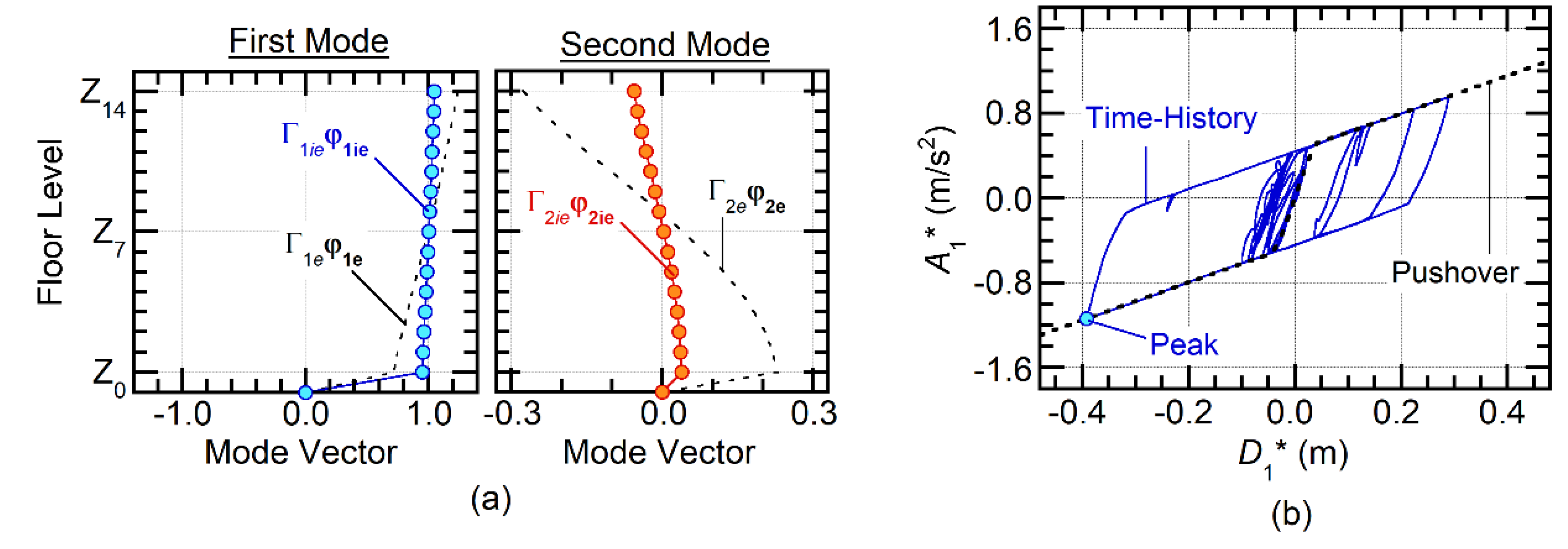
Figure 9 shows an example of the evaluated mode vector at peak and the first modal response of Model-14. The figures also show the relationship of the equivalent acceleration nA1* versus equivalent displacement nD1* calculated from pushover analysis results (Equations (4) and (17)):
Figure 9a shows that the first mode vector of Model-14 changes from the elastic stage: the component of level Z0 is closer to 1.0 and the superstructure comes to behave as a rigid body. The figure also shows that all components of the second mode vector are smaller from the elastic stage. The relationship of A1*(t) versus D1*(t) obtained from time-history analysis is regular and similar to the normal bilinear hysteresis rule, and its peak point agrees with the pushover result, as shown in Figure 9b. A similar observation is made for Model-05, which is not shown in this paper.
Figure 10 compares the relationships of A1* versus D1* obtained from the pushover analysis results and the peak of nonlinear time-history analysis results. The peaks of all nonlinear time-history analysis results are plotted in the figure. It is seen that all peak plots agree well with the curve of nA1* versus nD1* obtained from the pushover analysis results.
It is concluded from the above results that the calculation of the nonlinear modal response gives good results. The nonlinear modal responses are investigated in detail in the following discussions. Note that since the superstructure comes to behave as a rigid body in the nonlinear stage, the relative displacement of the level Z0 is almost equal to the equivalent displacement D1*. Therefore, the maximum deformations of isolators are approximately 0.5 m (Model-05) and 0.6 m (Model-14), respectively. According to a catalog provided by Bridgestone Corporation [22], the minimum of the ultimate horizontal deformation of the isolator used in Model-05 is 0.648 m, while that of Model-14 is 0.720 m (ultimate shear strain of rubber = 400%). Therefore, the responses shown in this study are smaller than the ultimate value.
3.2.2. Comparison of the Modal Response
Figure 11 shows the time-history response of Model-14 (Art-S09, 100%). In the figure, the responses of the relative displacement and restoring force at the top (level Z14), middle (level Z7), and bottom (level Z0) are shown. Note that “total (All Modes)” is the response originally obtained from time-history analysis results (e.g., displacement vector d(t) and restoring force vector fR(t)) while “First mode” is the response vector of the first mode (e.g., d1(t) and fR1(t)).
It is clear that, in terms of the relative displacement shown in Figure 11a, the first modal response agrees well with the total response. This confirms that the relative displacement response of Model-14 is governed by the first mode. However, this observation is different from that for the restoring force shown in Figure 11b, where the difference between the first modal response and the total response is notable at levels Z14 and Z0 and negligibly small at level Z7. This implies that the effect of the second and higher modal responses are significant in the restoring force, especially the top and bottom floor. A similar observation can be found in Model-05.
Figure 12 compares the modal responses at the top of Model-14 (Art-S09, 100%). The figures compare the relative displacement (d1(t), d2(t), and dh(t)) and restoring force (fR1(t), fR2(t), and fRh(t)). In terms of the relative displacement, the first modal response is the most pronounced and the second and higher modal responses are negligibly small, as shown in Figure 12a. In contrast, for the restoring force, the second modal response is more pronounced than the first modal response (Figure 12b).
Note that the higher modal response of the restoring force is smaller than the first and second modal responses. Therefore, the contribution of the higher modal response may be neglected for the approximation of the restoring force response of the base-isolated building models studied herein.
3.2.3. Simultaneity of the Peak Modal Response
The important issue in determining the proper horizontal force distribution used in the pushover analysis is the combination of the first and second modal responses. This section discusses the simultaneity of the peaks of the two modal responses.
The factor of simultaneity of the peaks of the two modal responses, γ, is defined as:
where, tpeak is the time at which |A1*(t)| reaches a maximum value, A1*max, and A2*max is the maximum value of |A2*(t)|. Using the factor γ, the horizontal force distribution, p, may expressed as:
Figure 13 shows the orbit of normalized acceleration of the two modal responses, A1*(t) / A1*max and A2*(t) / A2*max, for Model-05. The points at t = tpeak are plotted using the symbol “●”. It is seen that the range of γ is approximately between −1/2 and 1/2, i.e., most of the symbols “●” in the figure are distributed at A1*(t) / A1*max = ±1, −1/2 ≤ A2*(t) / A2*max ≤ 1/2. There are no plots corresponding to γ = ±1. No noticeable difference due to the intensity of ground motion or series (Art-S/L series) was observed.
Figure 14 shows the orbit of normalized acceleration of the two modal responses for Model-14. Most of the plots “●” in the figure are distributed at A1*(t) / A1*max = ±1, −1/2 ≤ A2*(t) / A2*max ≤ 1/2, and no plots correspond to γ = ±1. However, there are plots outside the range −1/2 ≤ A2*(t) / A2*max ≤ 1/2, especially when the intensity of ground motion is 50% (4 plots/12 analyses in Art-S series 50%, 3 plots/12 analyses in Art-L series).
It is concluded from the above investigation that the peaks of the first and second modal responses rarely occur simultaneously, although there is a certain level of contribution of the second modal response when the maximum first modal response occurs. Therefore, the value γ = ±1 may lead to overestimation while the value γ = 0 may lead to underestimation. The proper value of γ may be taken as 1/2. However, as shown in the case of Model-14 when the intensity of ground motion is 50%, the value of γ may be taken as larger than 1/2 for the conservative prediction of the maximum member force. It is interesting to note that Rahmani et al. had reached a similar conclusion in their research, that the contribution of the second mode should be factored by 0.5 for the improvement of accuracy in upper stories, in their improved upper-bound pushover analysis for the traditional moment-resisting frame structures [30].
4. Prediction of the Maximum Seismic Member Force in a Superstructure
This section proposes a set of pushover analyses considering the combination of the first and second modal responses. The predicted maximum member forces are then compared with the nonlinear time-history analysis results.
4.1. Proposal of a Set of Pushover Analyses
The procedure for a set of pushover analyses is described as follows. Note that the basic idea of a set of pushover analyses herein is the same as mode-adaptive bidirectional pushover analysis (MABPA) proposed previously by the author [24,29] for the consideration of combination of bidirectional excitation.
- Calculate a set of horizontal-force distributions p+ and p− in terms of the first- and second-mode vectors at D1*max:
- Perform the pushover analysis using the invariant force distributions p+ and p− (termed Pushover 1 and 2, respectively) until the equivalent displacement nD* calculated as:reaches D1*max.
- Determine the maximum response from the envelope of Pushover 1 and 2, i.e., the maximum relative displacement, the maximum restoring force, and the maximum member forces are obtained as the maximum value of the results of Pushover 1 and 2.
Note that Pushover 1 and 2 are carried out using the same model as the nonlinear time-history analysis by the same computer code. To investigate the accuracy of the proposed set of pushover analyses, the “exact” values of D1*max, A1*max and A2*max are used. The value D1*max used in the following section is taken as the mean of the peak modal response D1*peak obtained from the calculation of modal responses for 12 waves in each series. Similarly, the values A1*max and A2*max used in this section are taken as the mean of the maximum modal response obtained from the calculation of modal responses. The procedure for predicting D1*max, A1*max, and A2*max is not discussed in this paper.
The parameter γ, an important parameter considering the combination of the first and second modal responses, is set at 0, 1/2, 3/4, and 1. Note that the case γ = 0 is the case in which only the contribution of the first modal response is considered while the case γ = 1 is the case in which the maximum responses of the first and second modes are assumed to occur simultaneously. As discussed in the previous section, the case γ = 0 may result in underestimation while the case γ = 1 may result in overestimation.
4.2. Predicted Results and Comparison
4.2.1. Calculated Force Distribution
Figure 15 and Figure 16 respectively, show examples of calculated horizontal-force distributions for Models 05 and 14.
Stronger horizontal forces are applied to the lower floors in the force distribution p+ while stronger horizontal forces are applied to the upper floors in force distribution p−. Note that in the case that γ = 3/4 or 1, the horizontal forces applied to the top and bottom floors are opposite in sign. This is more pronounced for Model-14 than for Model-05.
4.2.2. Relative Displacement at Each Floor
Figure 17 compares the peak relative displacement of Model-05 for Art-S and -L series. The average, maximum, and minimum results of nonlinear time-history analysis are shown for each series and intensity of ground motion. It is seen that the pushover analysis results agree well with the average of the time-history analysis results, and the difference due to different values of γ is negligibly small.
Figure 18 compares the peak relative displacement of Model-14. Similar to the case for Model-05, the pushover analysis results agree well with the average of the time-history analysis results, although the difference due to different values of γ is noticeable at levels Z0 and Z 14.
4.2.3. Restoring Force at Each Floor
Figure 19 compares the peak restoring force of Model-05. It is seen that, in the case of γ = 0, the restoring force is underestimated except at level Z2. The results in the case γ = 1/2 are close to the average of the time-history analysis results, although the restoring force is underestimated at level Z5 when the ground motions are from the Art-S series. The results in the case γ = 3/4 are larger than the average of the time-history analysis results for all floors, and results in the case γ = 1 are larger than the maximum of time-history analysis results.
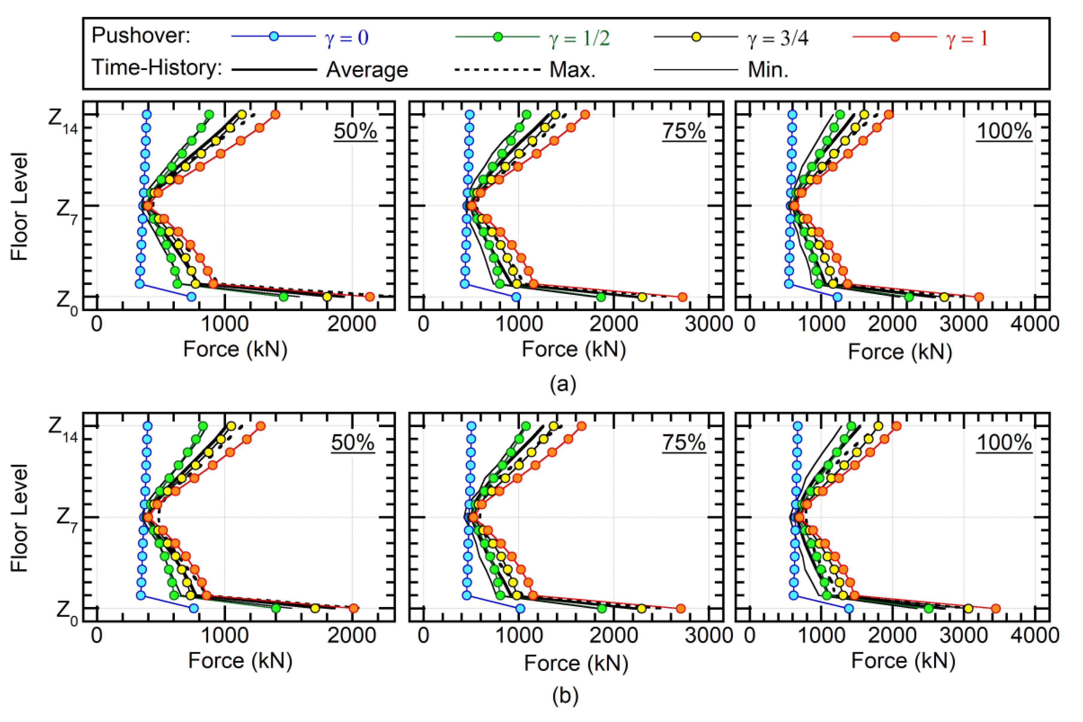
Figure 20 compares the peak restoring force for Model-14. Similar to the findings for Model-05, in the case γ = 0, the restoring force is underestimated except at level Z7. In the case γ = 1/2, the results are lower than the average of the time-history analysis results when the ground motion intensity is 50% or 75%. The results in the case γ = 3/4 are close to the average of the time-history analysis results for all floors when the ground motion intensity is 50% or 75%. The results in the case γ = 1 are larger than the maximum of time-history analysis results, except for level Z7.
4.2.4. Shear Force of Column
Figure 21 compares the maximum shear force of column X2Y2 in Model-05 while Figure 22 compares that in Model-14.
For Model-05, as shown in Figure 21, in the case γ = 0, both the maximum shear force and bending moment of column X2Y2 are underestimated in all stories. The results in the case γ = 1/2 are closer to the average of the time-history analysis results, although there is underestimation for the upper stories when the ground motion intensity is 50% or 75%. The estimation is conservative in the case γ = 3/4 but larger than the maximum of time-history analysis results in the case γ = 1.
Similar observations are presented for Model-14 in Figure 22, i.e., there are underestimations in the case γ = 0 and overestimations in the case γ = 1. Better estimations (closer to the average of the time-history analysis results) are obtained in the case γ = 1/2 or 3/4. It is noted that, when the ground motion intensity is 50%, the estimation is better in the case γ = 3/4 than in the case γ = 1/2, in which the estimation is lower than the average of the time-history analysis results. This finding is consistent with the observation in Figure 14.
4.3. Accuracy of the Proposed Procedure
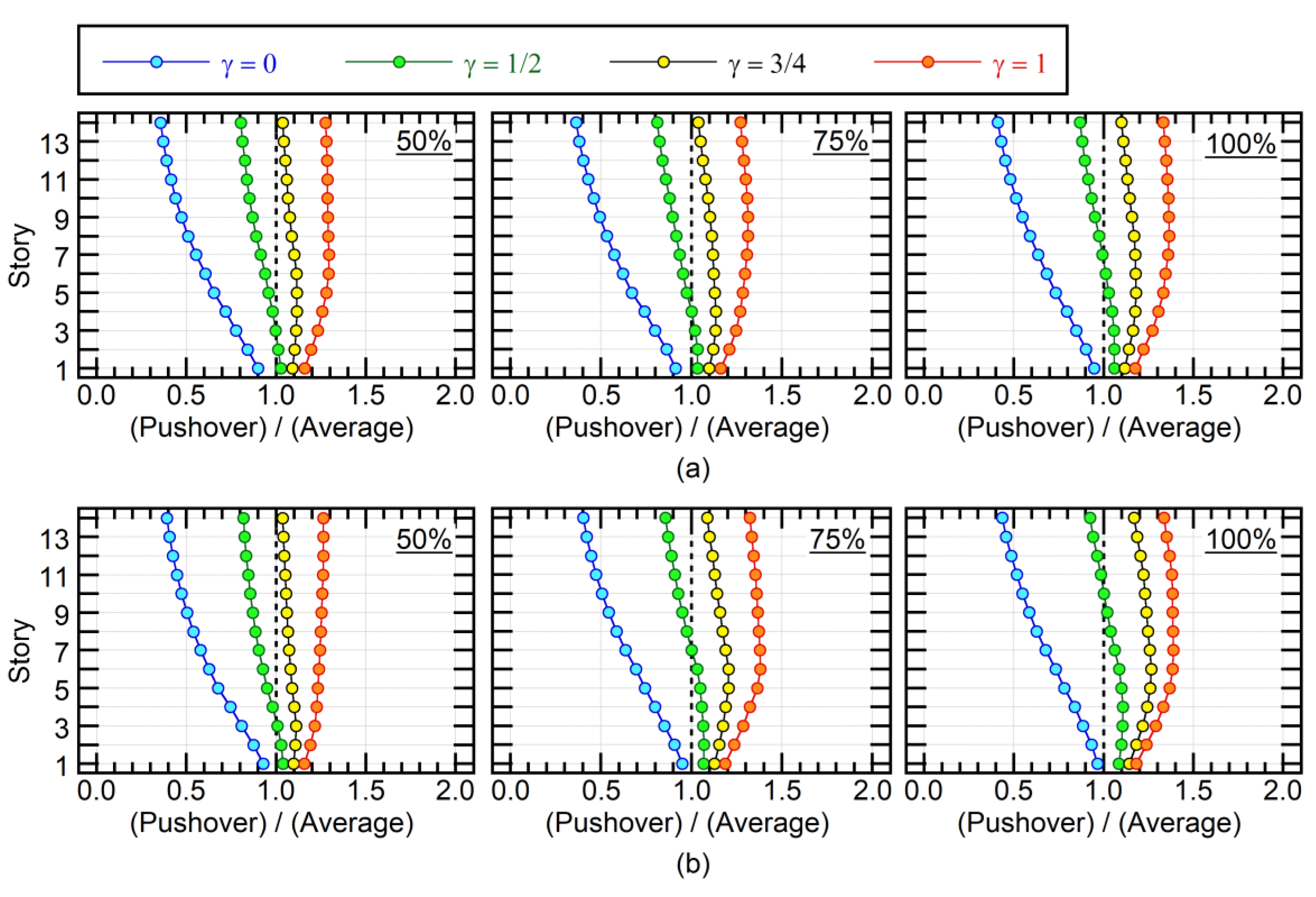
The ratio of the maximum shear force of column X2Y2 estimated in pushover analysis to the average time-history analysis result is used to investigate the accuracy of the proposed set of pushover analyses.
Figure 23 compares the accuracy of the pushover analyses results for Model-05 in terms of γ. It is seen that among the four cases, the case γ = 1/2 has the ratio closest to 1.0, except when the input ground motion is 50% of the Art-S series. In the case γ = 3/4, the estimations are conservative for all intensities of ground motions.
Figure 24 compares the accuracy of the pushover analyses results for Model-14 in terms of γ. It is seen that the estimations are conservative for all intensities of ground motions in the case γ = 3/4 while the member forces may be underestimated for the upper stories in the case γ = 1/2.
In conclusion, the maximum member force can be satisfactorily estimated adopting the proposed set of pushover analyses, by considering the combination of the first and second modal responses properly. As far as for the limited analysis results shown herein, reasonably conservative estimations are made in the case γ = 3/4. The member force is underestimated in the case γ = 0, where only the contribution of the first modal response is considered. In the case γ = 1, for which the peaks of the first and second modal responses are assumed to occur simultaneously, the member force is overestimated. The case γ = 1/2 may have the estimation closest to the average of the nonlinear time-history analysis results, however, results may be underestimated for upper stories.
5. Discussions and Conclusions
The maximum seismic member forces of five- and fourteen-story reinforced concrete base-isolated frame buildings were predicted by adopting pushover analysis. The main contributions and conclusions of the study are as follows.
- The calculation procedure for the nonlinear modal response was applied to the base-isolated frame buildings studied herein. Results show that the procedure works well for base-isolated buildings, i.e., the peak response of the first modal response agrees well with the results of pushover analysis, and the hysteresis rule of the first modal response is well regular and similar to normal bilinear behavior.
- The first modal response is predominant in the relative displacement responses of the base-isolated building models at all floor levels. In contrast, the contribution of the second modal response is important in the restoring force responses at the top and bottom floors of the base-isolated building models. Therefore, to determine the proper horizontal force distribution used in the pushover analysis, the combination of the first and second modal responses is an important issue.
- The peaks of the first and second modal responses rarely occur simultaneously, although there is a certain level of contribution of the second modal response when the maximum first modal response occurs. The factor of the simultaneity of the two modal responses, γ, approximately ranges between −1/2 and 1/2, however, there are cases that the absolute value of γ exceeds 1/2.
- The accuracy of the proposed set of pushover analyses for the prediction of the maximum member force was verified by nonlinear time-history analysis. Results show that the maximum member force can be satisfactorily predicted by considering the combination of the first and second modal responses properly. The limited numerical investigation herein revealed that the case γ = 3/4 provides reasonably conservative estimations. The case γ = 1/2 may provide the closest estimation to the average of nonlinear time-history analysis results, however, it may underestimate results in upper stories.
One of the contributions in this paper the author should emphasize is the proposal of a set of pushover analysis considering a) the changing of the first mode’s shape in each nonlinear stage, and b) the combination of the first and second modal responses. As is shown in Section 3.2.1, the mode shape at the peak response is changed significantly from the elastic range. This is because the nonlinearity of the isolated layer significantly affects the mode shape in case of the base-isolated buildings with LRB and hysteresis dampers. Besides, as is shown in Section 3.2.2, the contribution of the second modal response is significant to the restoring force acting at the top and bottom floors. In case of base-isolated buildings, the effective modal mass of the first mode is almost 100% of the total mass of the superstructure, and hence, the response of base-isolated building is expected to be governed by the first mode. The finding shown in Section 3.2.2 reveals that it is not true according to the restoring force in the top and bottom floors. Therefore, those points are essential for the better prediction of the peak response (e.g., displacement and member forces) for the base-isolated buildings by the nonlinear static analysis.
The procedure for predicting the peak response of each modal response was not discussed in this paper. The author believes that the nonlinear time-history analysis of the equivalent SDOF models can be applied to the prediction of the first modal response, as for ordinary nonlinear static procedures, or that the equations already proposed by Kilar and Koren [14] may simply be used. However, the prediction of the peak response for the second modal response would be more difficult because the change in the effective modal mass is appreciable owing to the change in the second mode vector. Another issues regarding in this topic is the applicability of the proposed set of pushover analyses to the base-isolated buildings with structural wall: as is well known in the seismic design of traditional earthquake-resistant structures, the seismic forces acting at the structural wall significantly affects the higher mode response in the case of a dual system (moment-resting frame with structural wall). The structural wall may also be used in base-isolated buildings for stiffening the superstructure, such as structural core wall of tall buildings. In such cases, the contribution of the second and higher modal response to seismic force in each member is a very complicated problem. The author wishes that the proposed set of pushover analyses may be one of the good solutions for such problems. Further works will address this issue.
Author Contributions
All contributions relating to this article were made by the first (single) author, except the preparation of the numerical model and editing of English as mentioned in the acknowledgements.
Funding
This research received no external funding.
Acknowledgments
The author thanks Tetsuya Ohno and Takuto Kawarazaki for helping establish the numerical model used in this paper and Glenn Pennycook, from Edanz Group (www.edanzediting.com/ac) for editing a draft of this paper.
Conflicts of Interest
The author declares no conflict of interest.
References
- Charleson, A.; Guisasola, A. Seismic Isolation for Architects; Routledge: London, UK; New York, NY, USA, 2017. [Google Scholar]
- Architectural Institute of JAPAN (AIJ). Design Recommendations for Seismically Isolated Buildings; Architectural Institute of Japan: Tokyo, Japan, 2016. [Google Scholar]
- Lee, D.G.; Hong, J.M.; Kim, J. Vertical distribution of equivalent static loads for base isolated building structures. Eng. Struct. 2001, 23, 1293–1306. [Google Scholar] [CrossRef]
- York, K.; Ryan, K.L. Distribution of lateral forces in base-isolated buildings considering isolation system nonlinearity. J. Eqrthq. Eng. 2008, 12, 1185–1204. [Google Scholar] [CrossRef]
- American Society of Civil Engineering (ASCE). Seismic Evaluation and Retrofit of Existing Buildings: ASCE Standard, ASCE/SEI41-17; American Society of Civil Engineering: Reston, VA, USA, 2017. [Google Scholar]
- Ordoñez, D.; Foti, D.; Bozzo, L. Comparative study of the inelastic response of base isolated buildings. Earthq. Eng. Struct. Dyn. 2003, 32, 151–164. [Google Scholar] [CrossRef]
- Kikuchi, M.; Black, C.J.; Aiken, I.D. On the response of yielding seismically isolated structures. Earthq. Eng. Struct. Dyn. 2008, 37, 659–679. [Google Scholar] [CrossRef]
- Cardone, D.; Flora, A.; Gesualdi, G. Inelastic response of RC frame buildings with seismic isolation. Earthq. Eng. Struct. Dyn. 2013, 42, 871–889. [Google Scholar] [CrossRef]
- Mazza, F.; Vulcano, A. Effects of near-fault ground motions on the nonlinear dynamic response of base-isolated r.c. framed buildings. Earthq. Eng. Struct. Dyn. 2012, 41, 211–232. [Google Scholar] [CrossRef]
- Fajfar, P. A nonlinear analysis method for performance-based seismic design. Earthq. Spectra 2000, 16, 573–592. [Google Scholar] [CrossRef]
- Kreslin, M.; Fajfar, P. The extended N2 method considering higher mode effects in both plan and elevation. Bull. Earthq. Eng. 2002, 10, 561–582. [Google Scholar] [CrossRef]
- Chopra, A.K.; Goel, R.K. A modal pushover analysis procedure for estimating seismic demands for buildings. Earthq. Eng. Struct. Dyn. 2013, 42, 871–889. [Google Scholar]
- Kilar, V.; Koren, D. Usage of Simplified N2 Method for Analysis of Base Isolated Structures. In Proceedings of the 14th World Conference on Earthquake Engineering, Beijing, China, 12–17 October 2008. [Google Scholar]
- Kilar, V.; Koren, D. Simplified inelastic seismic analysis of base-isolated structures using N2 method. Earthq. Eng. Struct. Dyn. 2010, 39, 967–989. [Google Scholar] [CrossRef]
- Kilar, V.; Koren, D. Seismic behaviour of asymmetric base isolated structures with various distributions of isolators. Eng. Struct. 2009, 31, 910–921. [Google Scholar] [CrossRef]
- Koren, D.; Kilar, V. The applicability of the N2 method to the estimation of torsional effects in asymmetric base-isolated buildings. Earthq. Eng. Struct. Dyn. 2011, 40, 867–886. [Google Scholar] [CrossRef]
- Providakis, C.P. Pushover analysis of base-isolated steel–concrete composite structures under near-fault excitations. Soil Dyn. Earthq. Eng. 2008, 28, 293–304. [Google Scholar] [CrossRef]
- Faal, H.N.; Poursha, M. Applicability of the N2, extended N2 and modal pushover analysis methods for the seismic evaluation of base-isolated building frames with lead rubber bearings (LRBs). Soil Dyn. Earthq. Eng. 2017, 98, 84–100. [Google Scholar] [CrossRef]
- Bhandari, M.; Bharti, S.D.; Shrimali, M.K.; Datta, T.K. Assessment of proposed lateral load patterns in pushover analysis for base-isolated frames. Eng. Struct. 2018, 175, 531–548. [Google Scholar] [CrossRef]
- Bhandari, M.; Bharti, S.D.; Shrimali, M.K.; Datta, T.K. Applicability of capacity spectrum method for base-isolated building frames at different performance points. J. Eqrthq. Eng. 2018, 1–30. Available online: www.tandfonline.com (accessed on 30 June 2019). [CrossRef]
- Japan Building Disaster Prevention Association (JBDPA). Kozo-Sekkei Buzai-Damnen Jirei-Shu (Structural Design Examples of Member Sections of Buildings); Japan Building Disaster Prevention Association: Tokyo, Japan, 2007. (in Japanese) [Google Scholar]
- Bridgestone Corporation. Seismic Isolation Product Line-Up Version 2017. Volume 1. Available online: https://www.bridgestone.com/products/diversified/antiseismic_rubber/pdf/catalog_201710.pdf (accessed on 3 August 2019).
- Nippon Steel Engineering Co. Ltd. Men-shin NSU Damper Line-Up. Available online: https://www.eng.nipponsteel.com/steelstructures/product/base_isolation/damper_u/lineup_du/ (accessed on 3 August 2019).
- Fujii, K. Pushover-based seismic capacity evaluation of Uto city hall damaged by the 2016 Kumamoto earthquake. Buildings 2019, 9, 140. [Google Scholar] [CrossRef]
- Wada, A.; Hirose, K. Elasto-plastic dynamic behaviors of the building frames subjected to bi-directional earthquake motions. J. Struct. Const. Eng. AIJ 1989, 399, 37–47. (In Japanese) [Google Scholar]
- Building Research Institute (BRI). BRI Strong Motion Network, Strong Motion Report, 2011/03/11 14:46 off Sanriku (M = 9.0, h = 24 km). Available online: http://smo.kenken.go.jp/index.php/report/201103111446 (accessed on 4 August 2019).
- Fujii, K.; Miyagawa, K. Nonlinear Seismic Response of A Seven-Story Steel Reinforced Concrete Condominium Retrofitted with Low-Yield-Strength-Steel Damper Columns. In Proceedings of the 16th European Conference on Earthquake Engineering, Thessaloniki, Greece, 18–21 June 2018. [Google Scholar]
- Kuramoto, H. Earthquake response characteristics of equivalent SDOF system reduced from multi-story buildings and prediction of higher mode responses. J. Struct. Const. Eng. 2004, 580, 61–68. (in Japanese). [Google Scholar] [CrossRef]
- Fujii, K. Prediction of the largest peak nonlinear seismic response of asymmetric buildings under bi-directional excitation using pushover analyses. Bull. Earthq. Eng. 2014, 12, 909–938. [Google Scholar] [CrossRef]
- Rahmani, A.Y.; Bourahla, N.; Bento, R.; Badaoui, M. An improved upper-bound pushover procedure for seismic assessment of high-rise moment resisting steel frames. Bull. Earthq. Eng. 2018, 16, 315–339. [Google Scholar] [CrossRef]
Figure 1.
Simplified structural plan and elevation (Model-05): (a) plan of levels Z1 to Z5, (b) plan of level Z0, and (c) elevation of frame Y2.
Figure 1.
Simplified structural plan and elevation (Model-05): (a) plan of levels Z1 to Z5, (b) plan of level Z0, and (c) elevation of frame Y2.
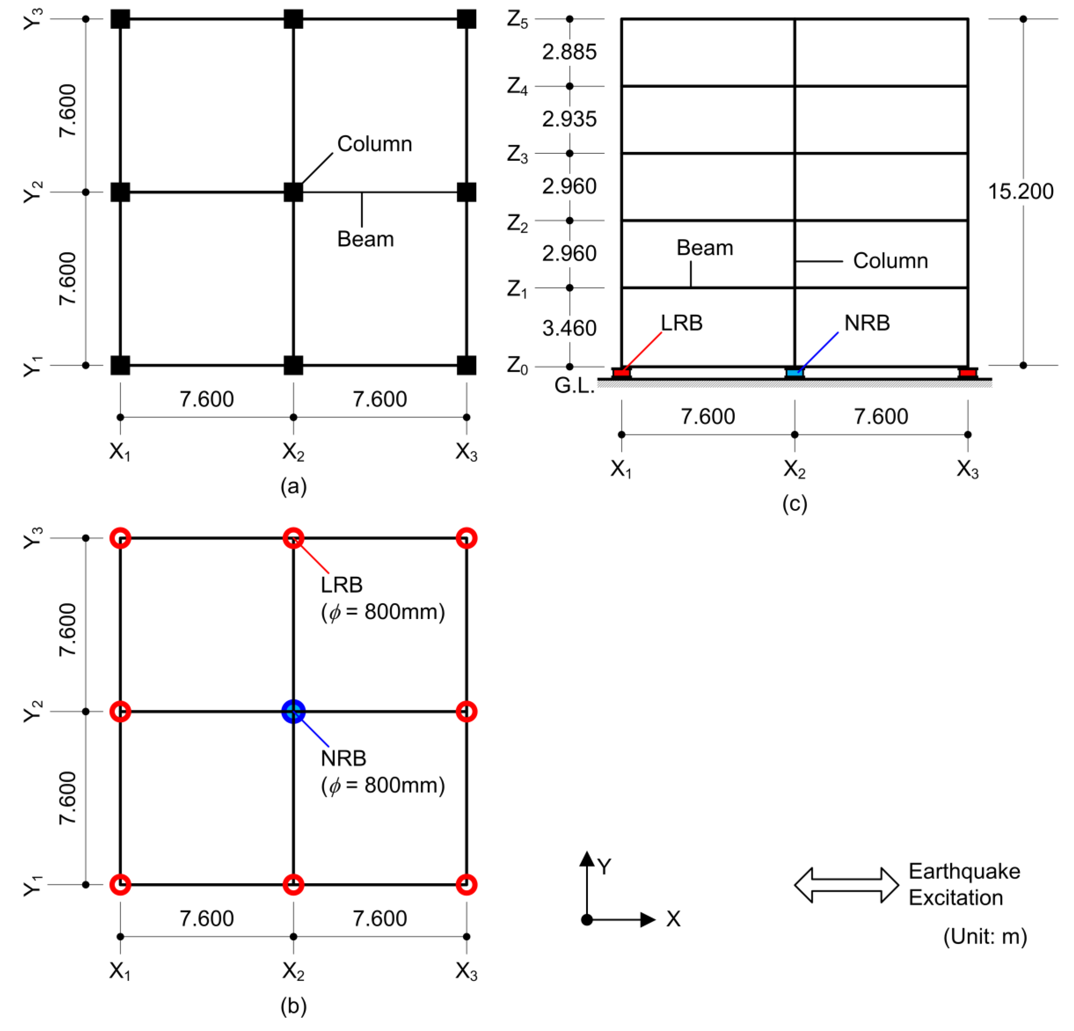
Figure 2.
Simplified structural plan and elevation (Model-14): (a) plan of levels Z1 to Z14, (b) plan of level Z0, and (c) elevation of frame Y2.
Figure 2.
Simplified structural plan and elevation (Model-14): (a) plan of levels Z1 to Z14, (b) plan of level Z0, and (c) elevation of frame Y2.
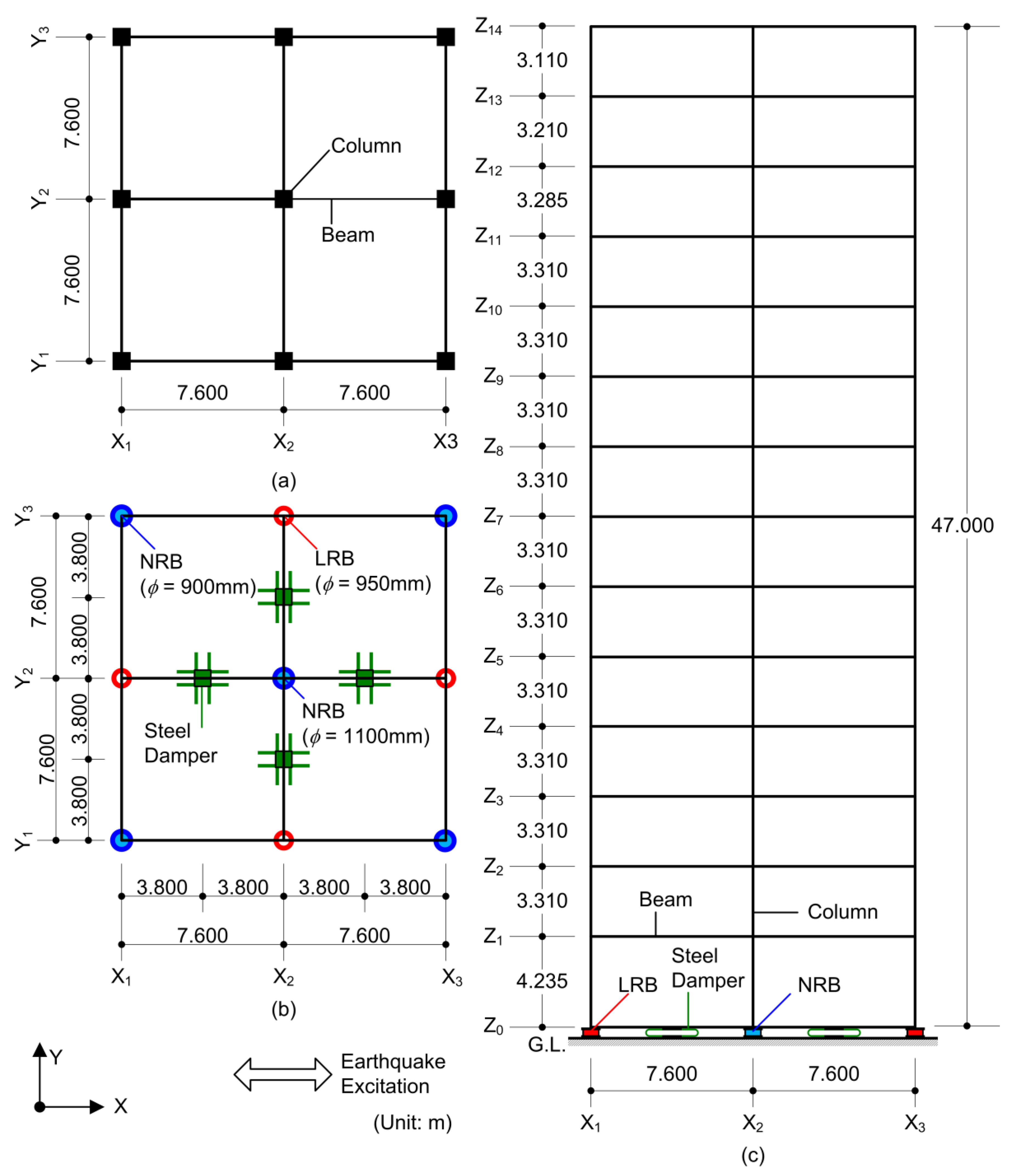
Figure 3.
Envelopes of the force–deformation relationship for isolators and damper: (a) natural rubber bearing (NRB), (b) lead-rubber bearing (LRB), and (c) steel damper.
Figure 3.
Envelopes of the force–deformation relationship for isolators and damper: (a) natural rubber bearing (NRB), (b) lead-rubber bearing (LRB), and (c) steel damper.
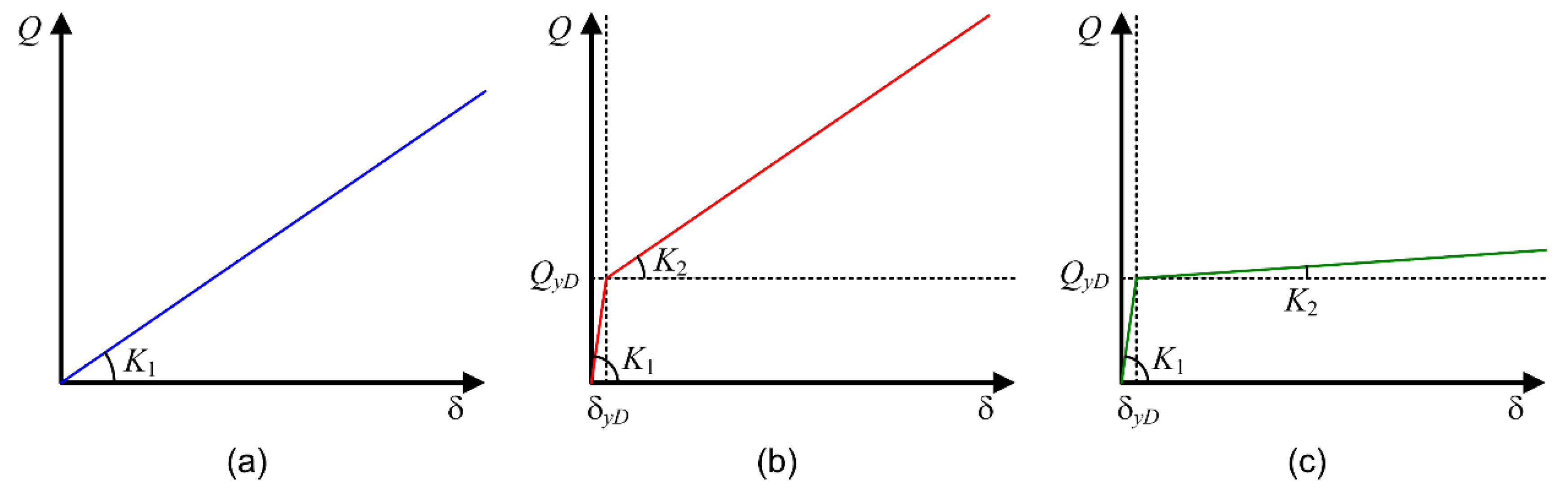
Figure 4.
Shapes of the first and second natural mode vectors of the building models in the elastic range: (a) Model-05 and (b) Model-14.
Figure 4.
Shapes of the first and second natural mode vectors of the building models in the elastic range: (a) Model-05 and (b) Model-14.
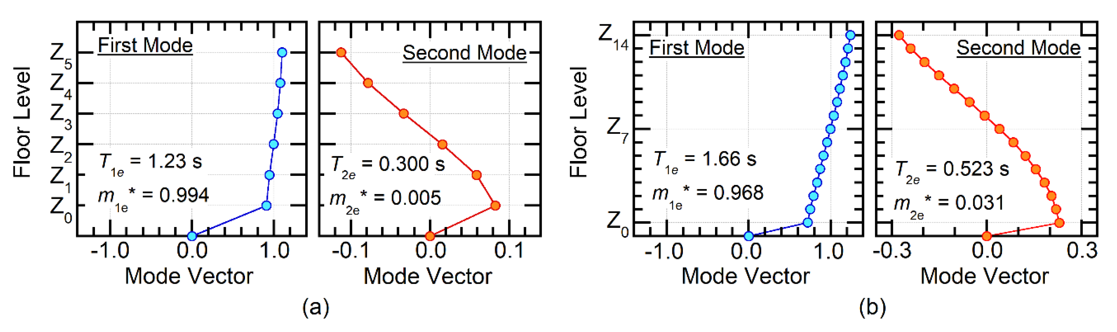
Figure 5.
Elastic pseudo acceleration spectrum of the generated artificial ground motions: (a) Art-S Series and (b) Art-L Series.
Figure 5.
Elastic pseudo acceleration spectrum of the generated artificial ground motions: (a) Art-S Series and (b) Art-L Series.

Figure 6.
Example wave of the generated artificial ground motion: (a) Art-S00 and (b) Art-L00.
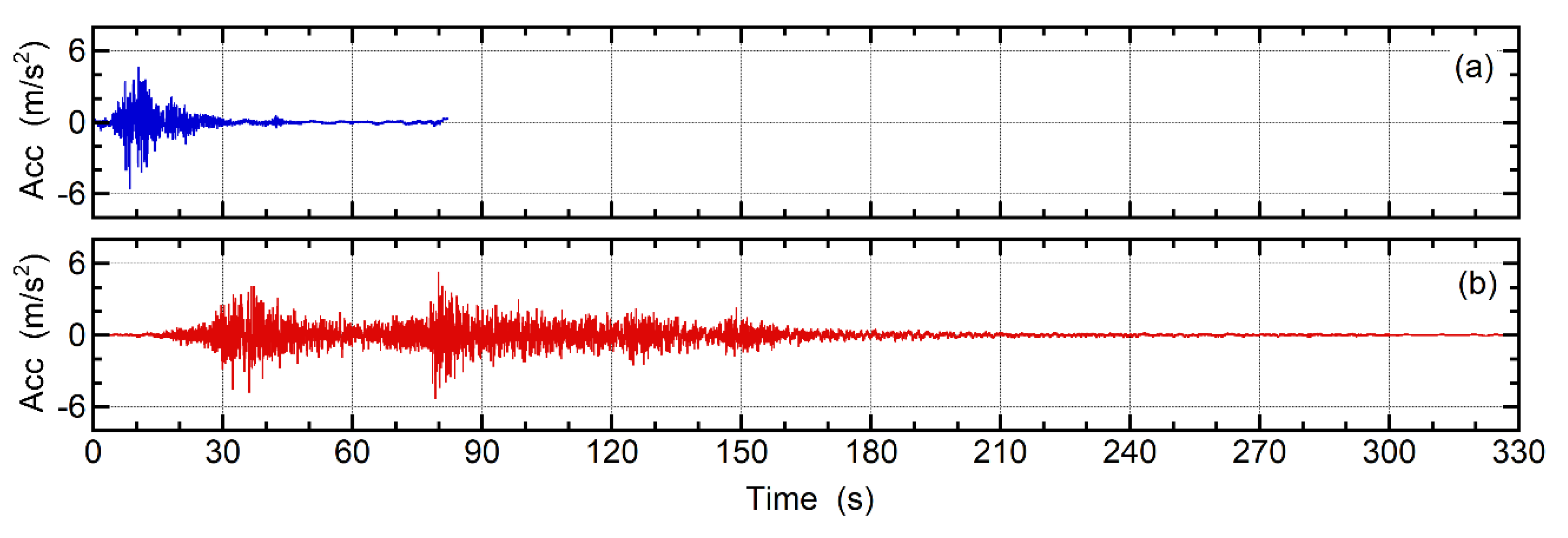
Figure 7.
Comparison of the 12 waves of the Art-S series: (a) 0 to 30 s and (b) 7 to 9 s.
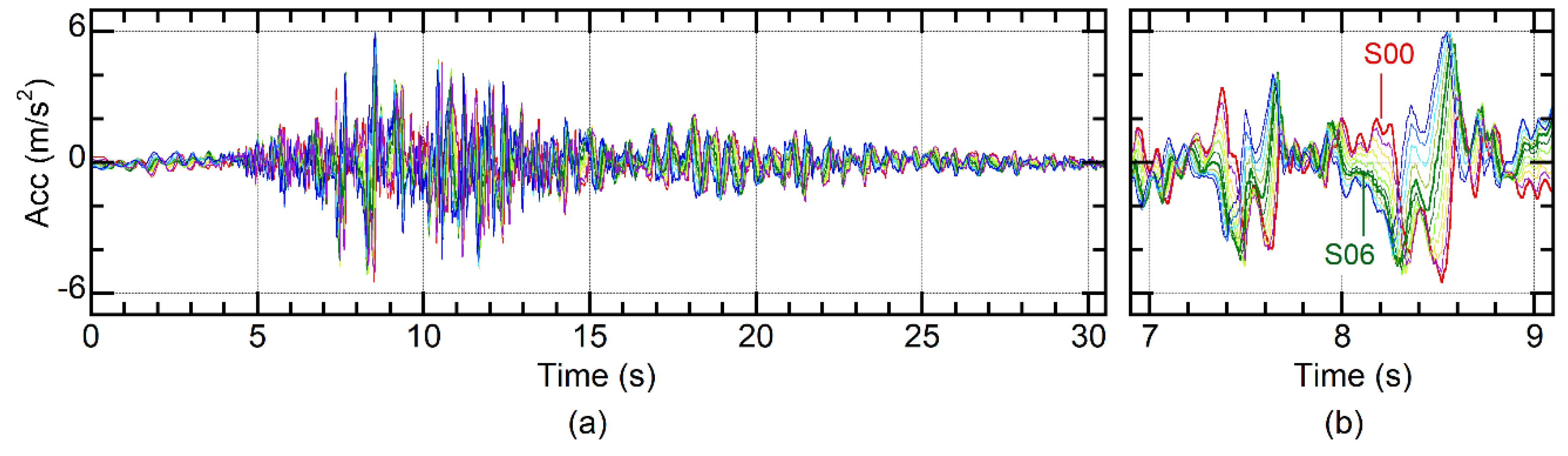
Figure 8.
The concept of the calculating modal response.
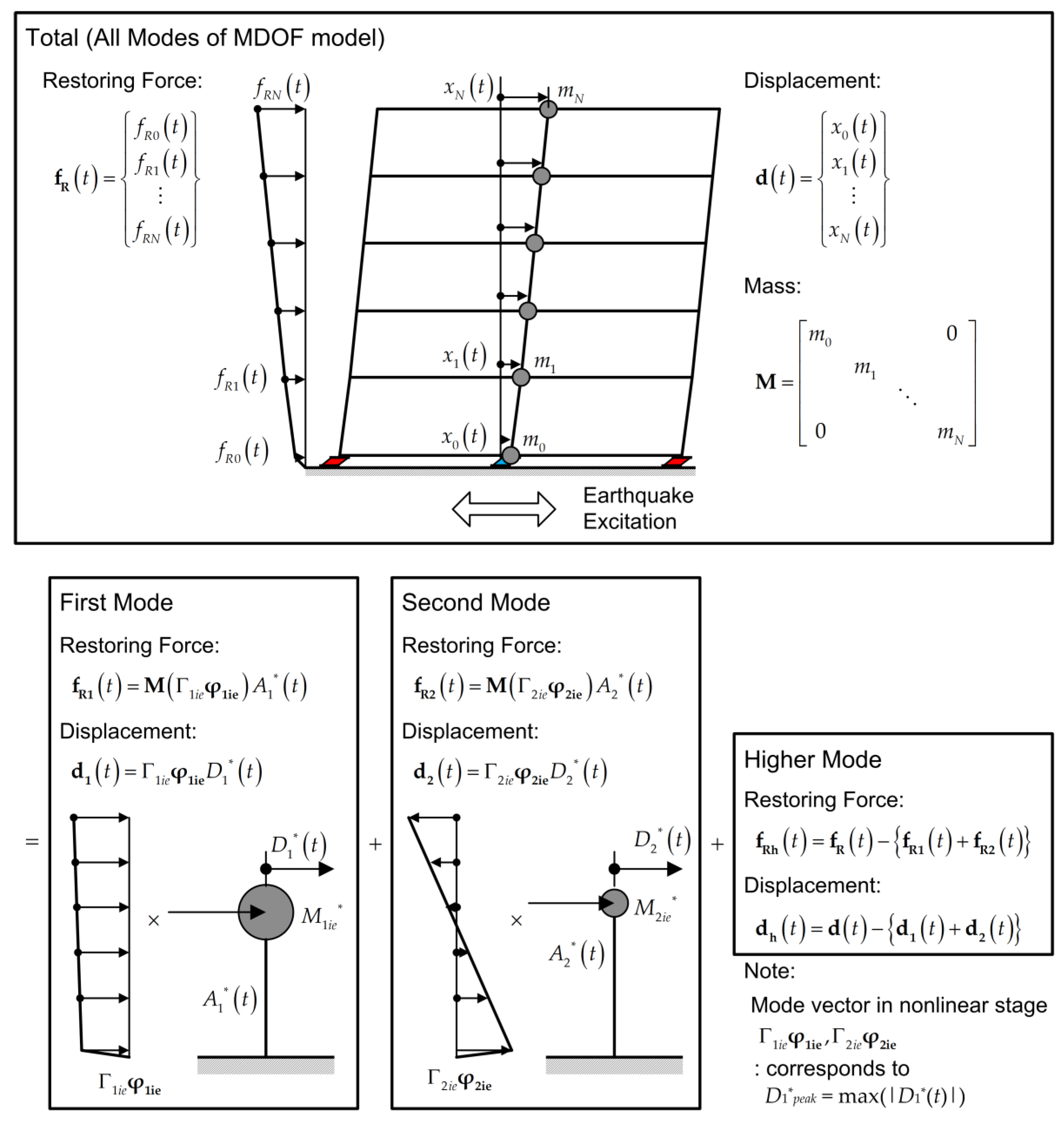
Figure 9.
Evaluated mode vector at the peak response and first modal response of Model-14 (Art-S03, 100%): (a) shape of the first and second mode vectors at the peak response and (b) comparison of the relationships of A1* versus D1* calculated from the nonlinear time-history analysis and pushover analysis results.

Figure 10.
Comparison of the relationships of A1* versus D1* calculated from the pushover analysis results and the peak of nonlinear time-history analysis: (a) Model-05 and (b) Model-14.
Figure 10.
Comparison of the relationships of A1* versus D1* calculated from the pushover analysis results and the peak of nonlinear time-history analysis: (a) Model-05 and (b) Model-14.
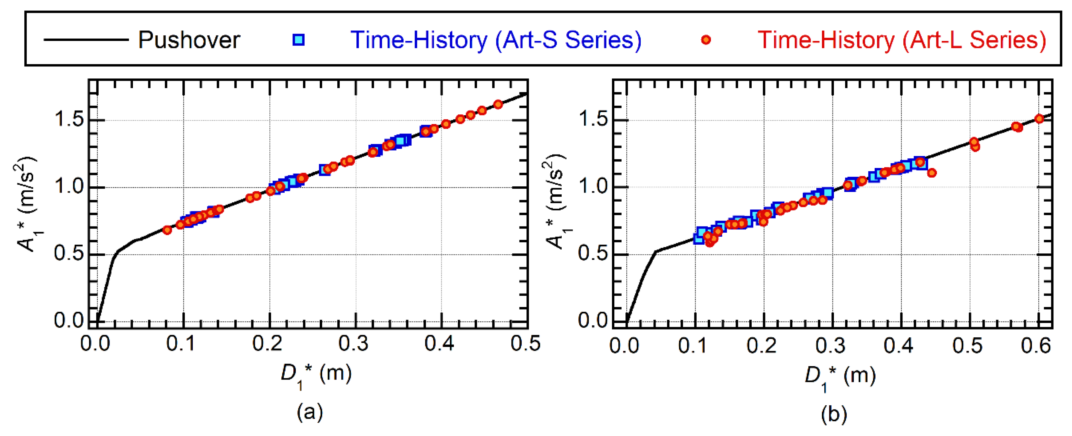
Figure 11.
Time-history response of Model-14(Art-S09, 100%): (a) relative displacement and (b) restoring force.
Figure 11.
Time-history response of Model-14(Art-S09, 100%): (a) relative displacement and (b) restoring force.
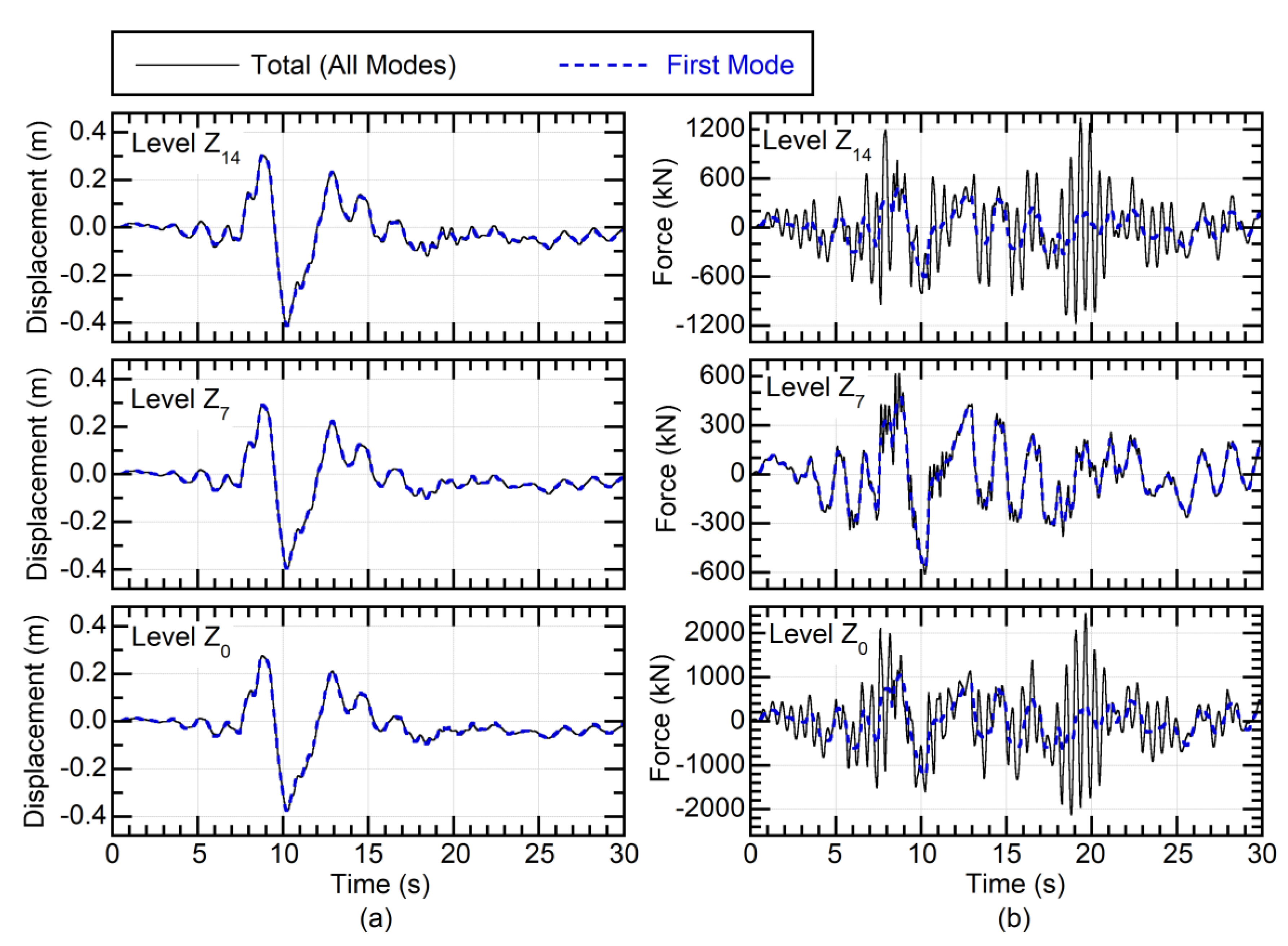
Figure 12.
Comparison of modal response of Model-14 at level Z14 (Art-S09, 100%): (a) relative displacement and (b) restoring force.
Figure 12.
Comparison of modal response of Model-14 at level Z14 (Art-S09, 100%): (a) relative displacement and (b) restoring force.

Figure 13.
Orbit of normalized equivalent acceleration (Model-05): (a) Art-S series and (b) Art-L series.
Figure 13.
Orbit of normalized equivalent acceleration (Model-05): (a) Art-S series and (b) Art-L series.
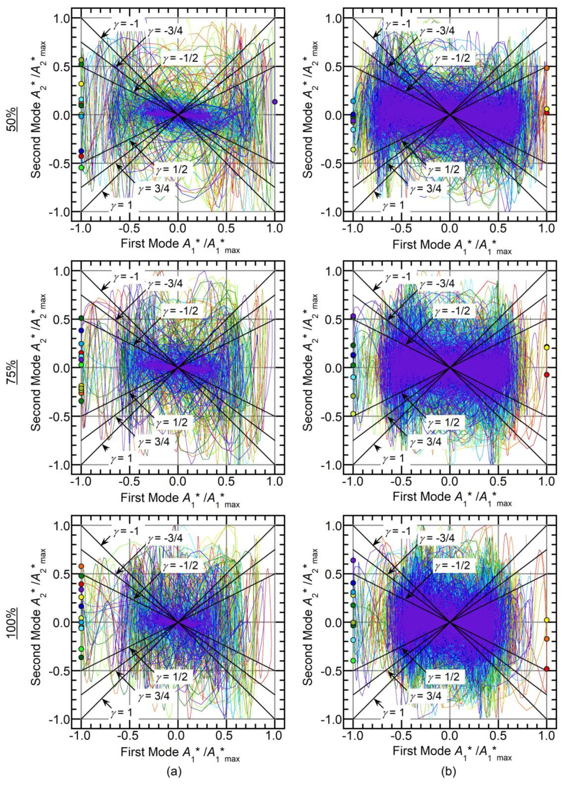
Figure 14.
Orbit of normalized equivalent acceleration (Model-14): (a) Art-S series and (b) Art-L series.
Figure 14.
Orbit of normalized equivalent acceleration (Model-14): (a) Art-S series and (b) Art-L series.
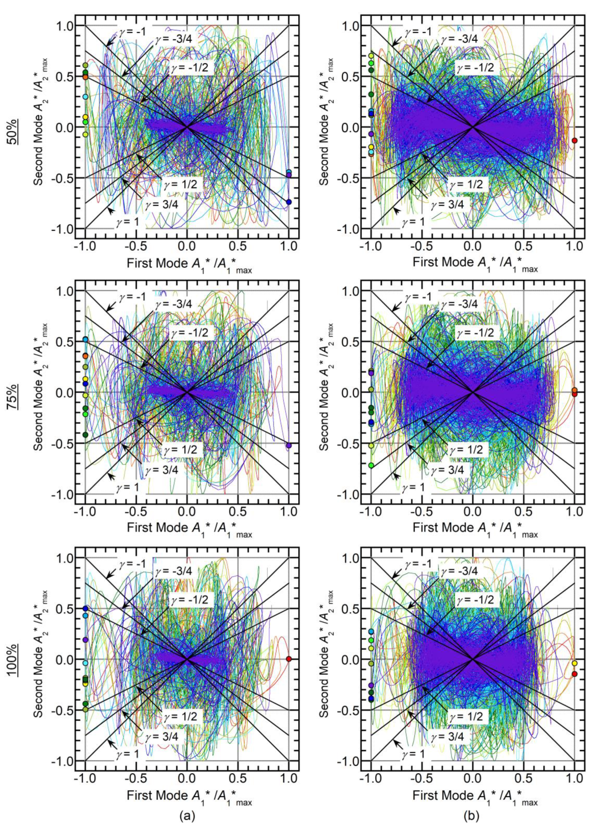
Figure 15.
Examples of calculated horizontal-force distributions for Model-05 (Art-S, 100%).
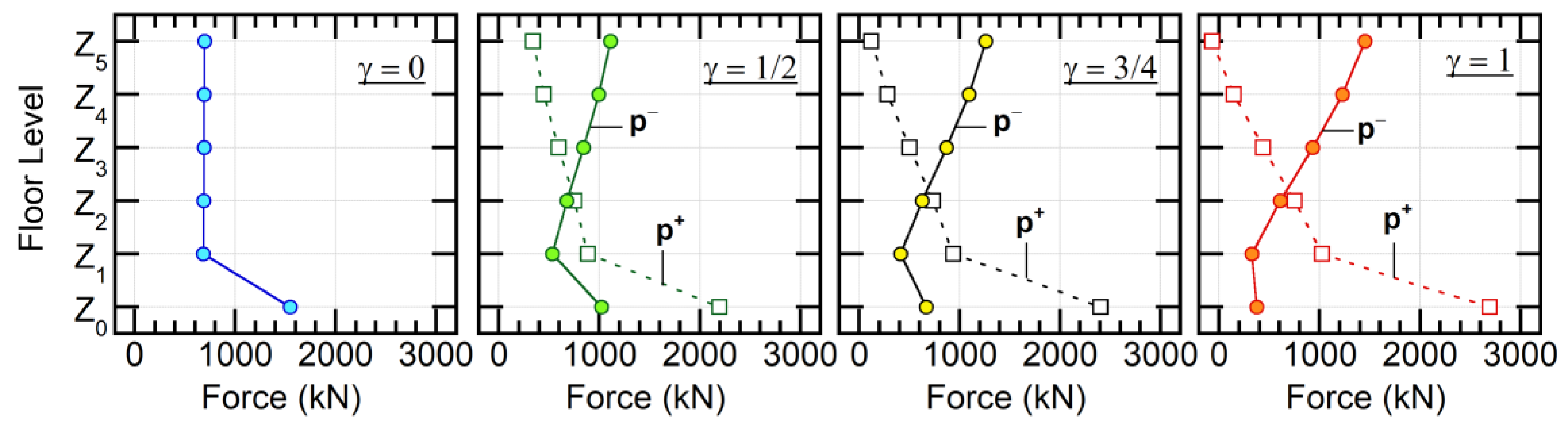
Figure 16.
Examples of calculated horizontal-force distributions for Model-14 (Art-S, 100%).
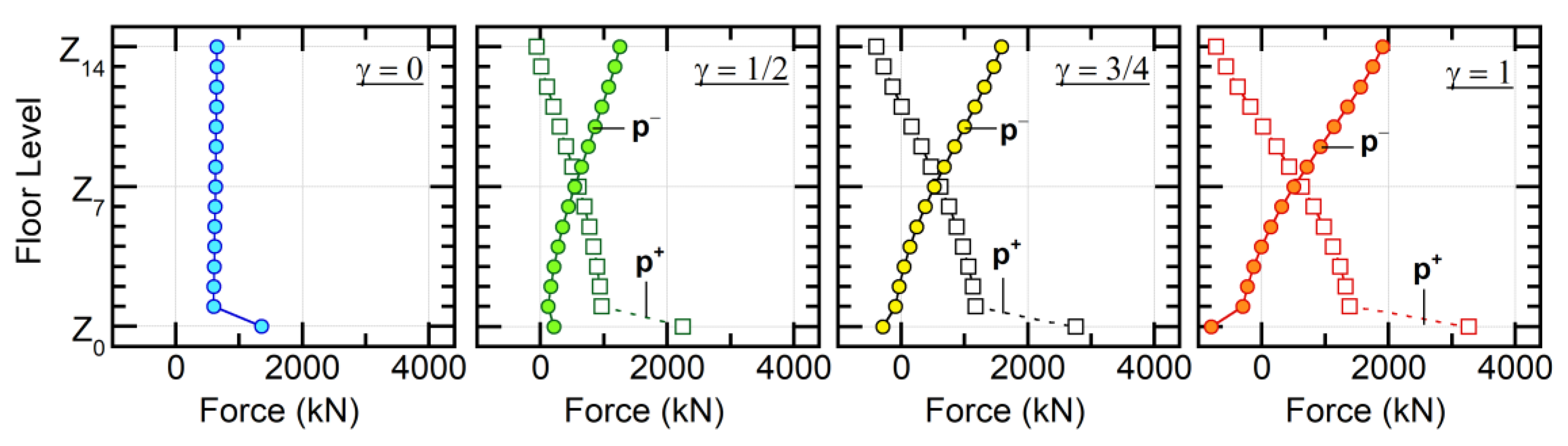
Figure 17.
Comparison of the peak relative displacement of Model-05: (a) Art-S series and (b) Art-L series.
Figure 17.
Comparison of the peak relative displacement of Model-05: (a) Art-S series and (b) Art-L series.
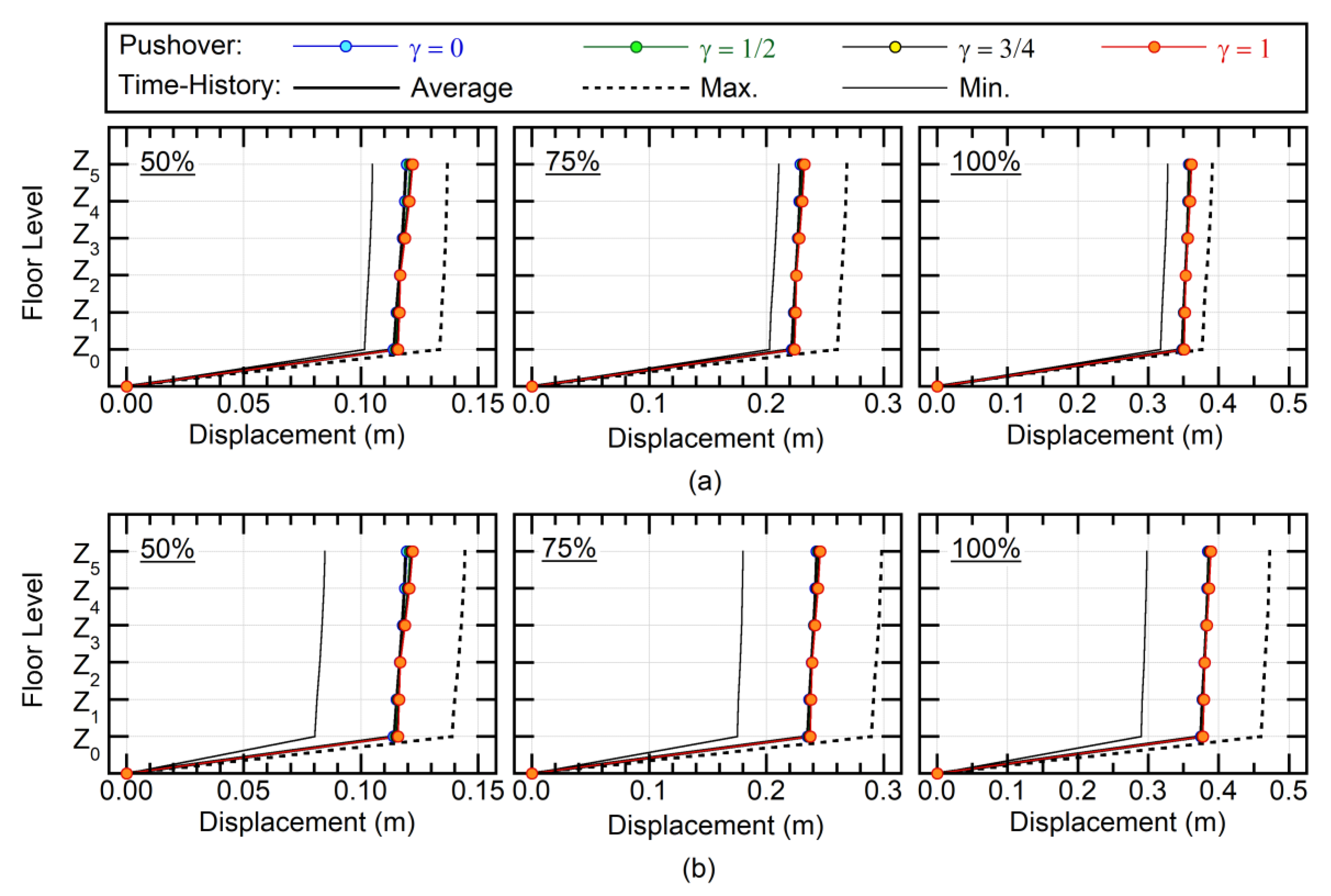
Figure 18.
Comparison of the peak relative displacement of Model-14: (a) Art-S series and (b) Art-L series.
Figure 18.
Comparison of the peak relative displacement of Model-14: (a) Art-S series and (b) Art-L series.

Figure 19.
Comparison of the peak restoring force for Model-05: (a) Art-S series and (b) Art-L series.
Figure 19.
Comparison of the peak restoring force for Model-05: (a) Art-S series and (b) Art-L series.

Figure 20.
Comparison of the peak restoring force for Model-14: (a) Art-S series and (b) Art-L series.
Figure 20.
Comparison of the peak restoring force for Model-14: (a) Art-S series and (b) Art-L series.

Figure 21.
Comparison of the maximum shear force of column X2Y2 in Model-05: (a) Art-S series and (b) Art-L series.
Figure 21.
Comparison of the maximum shear force of column X2Y2 in Model-05: (a) Art-S series and (b) Art-L series.
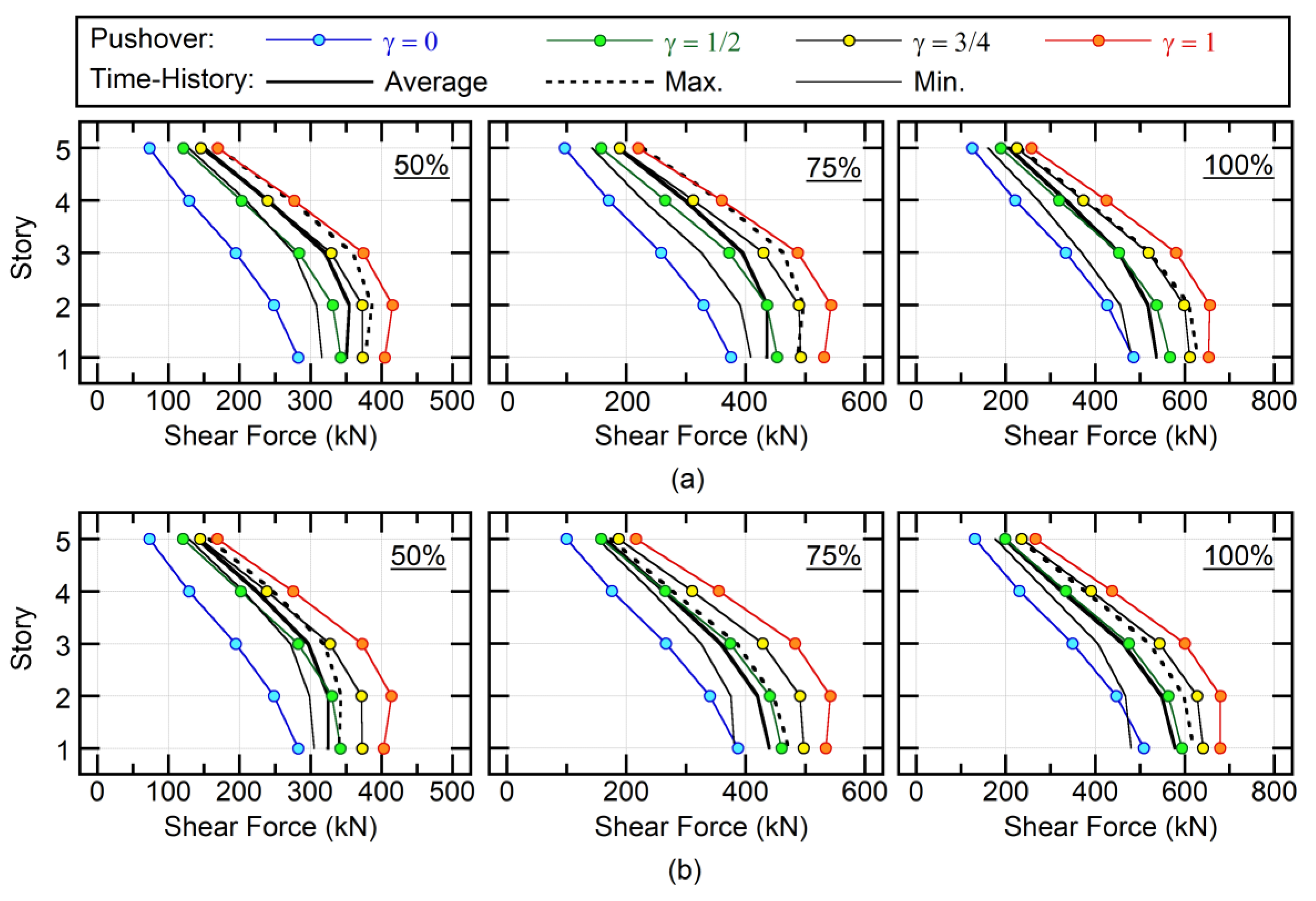
Figure 22.
Comparison of the maximum shear force of column X2Y2 in Model-14: (a) Art-S series and (b) Art-L series.
Figure 22.
Comparison of the maximum shear force of column X2Y2 in Model-14: (a) Art-S series and (b) Art-L series.
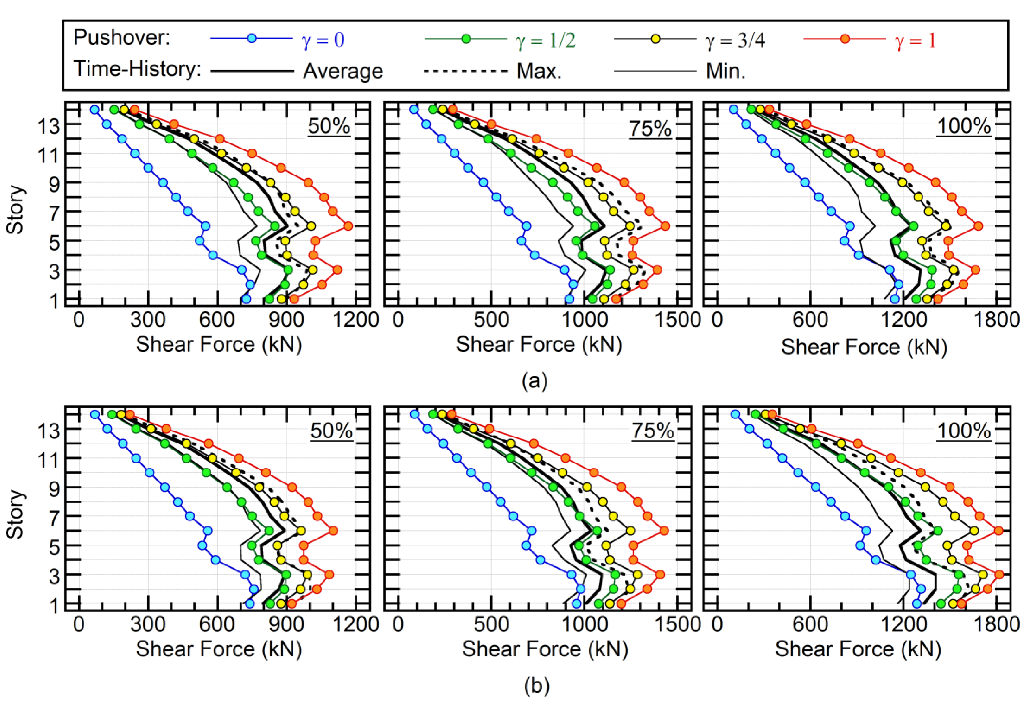
Figure 23.
Accuracy of the pushover analysis results in comparison with the average values of time-history analysis (Model-05, shear force of column X2Y2): (a) Art-S series and (b) Art-L series.
Figure 23.
Accuracy of the pushover analysis results in comparison with the average values of time-history analysis (Model-05, shear force of column X2Y2): (a) Art-S series and (b) Art-L series.
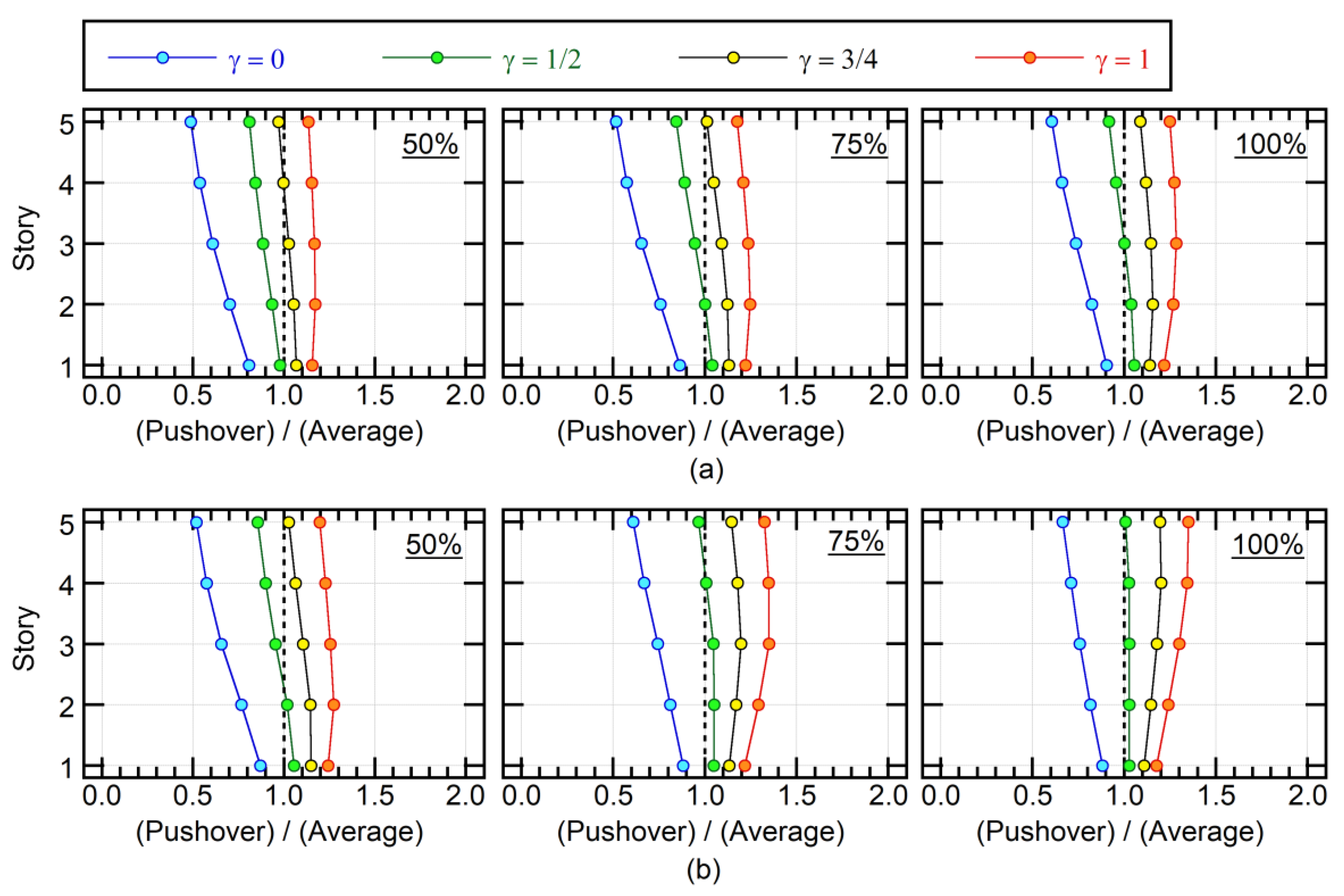
Figure 24.
Accuracy of the pushover analysis results in comparison with the average values of time-history analysis (Model-14, shear force of column X2Y2): (a) Art-S series and (b) Art-L series.
Figure 24.
Accuracy of the pushover analysis results in comparison with the average values of time-history analysis (Model-14, shear force of column X2Y2): (a) Art-S series and (b) Art-L series.


Table 1.
Member sections, compressive strength, and Young’s modulus of concrete for Model-05.
| Member | Section | Compressive Strength (MPa) | Young’s Modulus (MPa) |
|---|---|---|---|
| Beam (Z5) | 500 mm × 700 mm | 24 | 2.27 × 10⁴ |
| Beam (Z4) | 500 mm × 750 mm | ||
| Beam (Z1 to Z3) | 550 mm × 800 mm | ||
| Beam (Z0) | 750 mm × 1800 mm | ||
| Column (All) | 850 mm × 850 mm | 24 | 2.27 × 10⁴ |
Table 2.
Member sections, compressive strength, and Young’s modulus of concrete for Model-14.
| Member | Section | Compressive Strength (MPa) | Young’s Modulus (MPa) |
|---|---|---|---|
| Beam (Z14) | 550 mm × 900 mm | 24 | 2.27 × 10⁴ |
| Beam (Z13) | 550 mm × 1000 mm | ||
| Beam (Z12) | 600 mm × 1100 mm | 27 | 2.35 × 10⁴ |
| Beam (Z11) | 700 mm × 1150 mm | ||
| Beam (Z7 to Z10) | 700 mm × 1150 mm | 33 | 2.52 × 10⁴ |
| Beam (Z1 to Z6) | 700 mm × 1150 mm | 36 | 2.59 × 10⁴ |
| Beam (Z0) | 850 mm × 3000 mm | ||
| Column (13th to 14th Story) | 950 mm × 950 mm | 24 | 2.27 × 10⁴ |
| Column (11th to 12th Story) | 1000 mm × 1000 mm | 27 | 2.35 × 10⁴ |
| Column (7th to 10th Story) | 1050 mm × 1050 mm | 33 | 2.52 × 10⁴ |
| Column (1st to 6th Story) | 1100 mm × 1100 mm | 36 | 2.59 × 10⁴ |
Table 3.
Properties of selected isolators for Model-05.
| Type | Amount | Outer Diameter (mm) | Lead Plug Diameter (mm) | Shear Modulus (MPa) | Initial Stiffness K1 (MN/m) | Yield Strength QyD (kN) | Post Yield Stiffness K2 (MN/m) | Vertical Stiffness KV (MN/m) |
|---|---|---|---|---|---|---|---|---|
| NRB | 1 | 800 | − | 0.294 | 0.912 | − | − | 2800 |
| LRB | 8 | 800 | 200 | 0.385 | 13.0 | 250 | 1.00 | 2960 |
Table 4.
Properties of selected isolators for Model-14.
| Type | Amount | Outer Diameter (mm) | Lead Plug Diameter (mm) | Shear Modulus (MPa) | Initial Stiffness K1 (MN/m) | Yield Strength QyD (kN) | Post Yield Stiffness K2 (MN/m) | Vertical Stiffness KV (MN/m) |
|---|---|---|---|---|---|---|---|---|
| NRB | 4 | 900 | − | 0.441 | 1.56 | − | − | 3730 |
| NRB | 1 | 1100 | − | 0.441 | 1.89 | − | − | 4510 |
| LRB | 4 | 950 | 240 | 0.385 | 18.5 | 360 | 1.42 | 4210 |
Table 5.
Properties of selected steel dampers for Model-14.
| Amount | Initial Stiffness K1 (MN/m) | Yield Strength QyD (kN) | Post Yield Stiffness K2 (MN/m) |
|---|---|---|---|
| 4 | 19.2 | 608 | 0.32 |
© 2019 by the author. Licensee MDPI, Basel, Switzerland. This article is an open access article distributed under the terms and conditions of the Creative Commons Attribution (CC BY) license (http://creativecommons.org/licenses/by/4.0/).
Share and Cite
MDPI and ACS Style
Fujii, K. Prediction of the Maximum Seismic Member Force in a Superstructure of a Base-Isolated Frame Building by Using Pushover Analysis. Buildings 2019, 9, 201. https://doi.org/10.3390/buildings9090201
AMA Style
Fujii K. Prediction of the Maximum Seismic Member Force in a Superstructure of a Base-Isolated Frame Building by Using Pushover Analysis. Buildings. 2019; 9(9):201. https://doi.org/10.3390/buildings9090201
Chicago/Turabian StyleFujii, Kenji. 2019. "Prediction of the Maximum Seismic Member Force in a Superstructure of a Base-Isolated Frame Building by Using Pushover Analysis" Buildings 9, no. 9: 201. https://doi.org/10.3390/buildings9090201
Note that from the first issue of 2016, this journal uses article numbers instead of page numbers. See further details here.