Impacts of Microclimate Conditions on the Energy Performance of Buildings in Urban Areas


Abstract

1. Introduction
2. Background
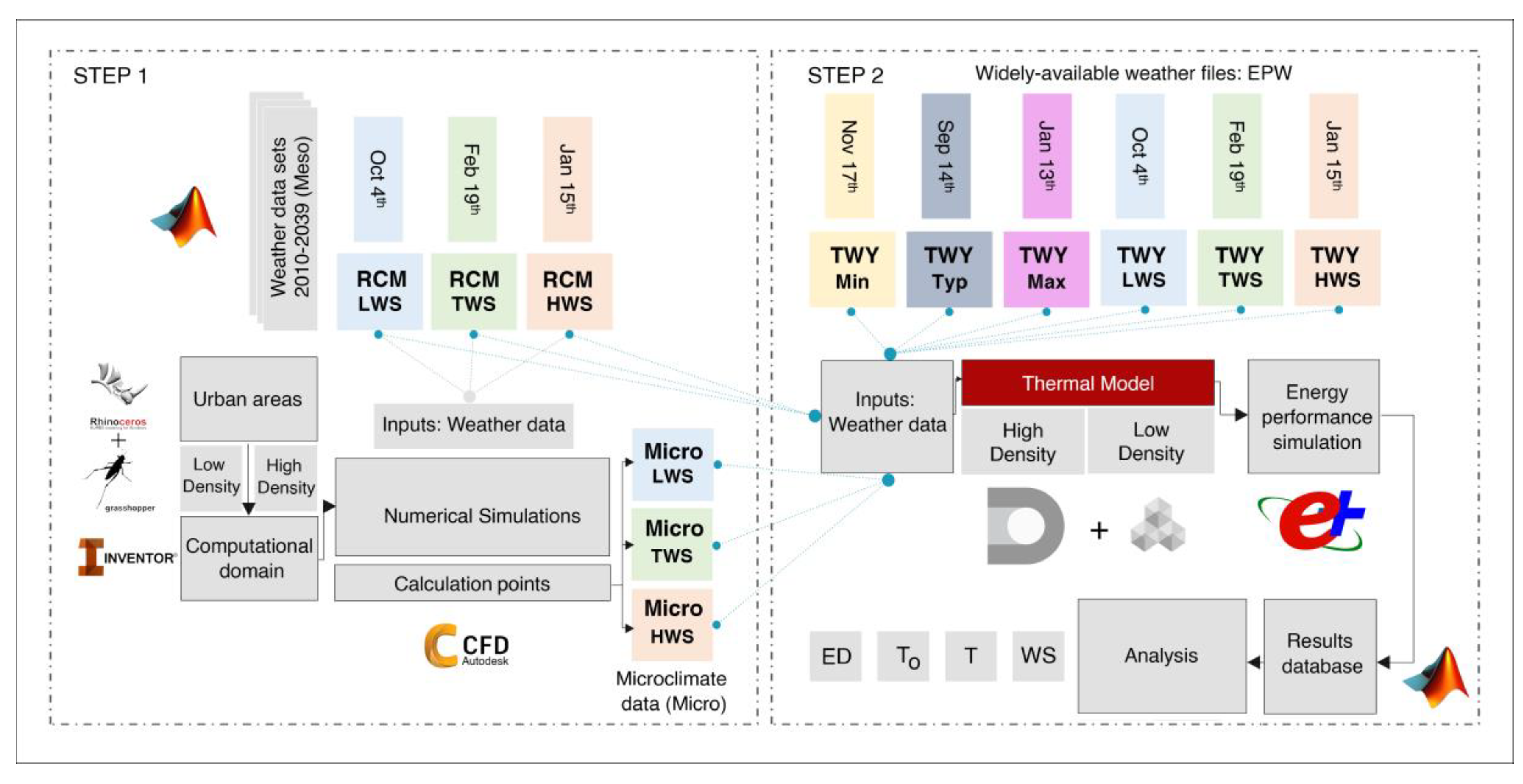
3. Methodology
3.1. Modeling Urban Areas
3.2. Weather Data Sets
3.3. CFD and EPS
4. Results and Discussion
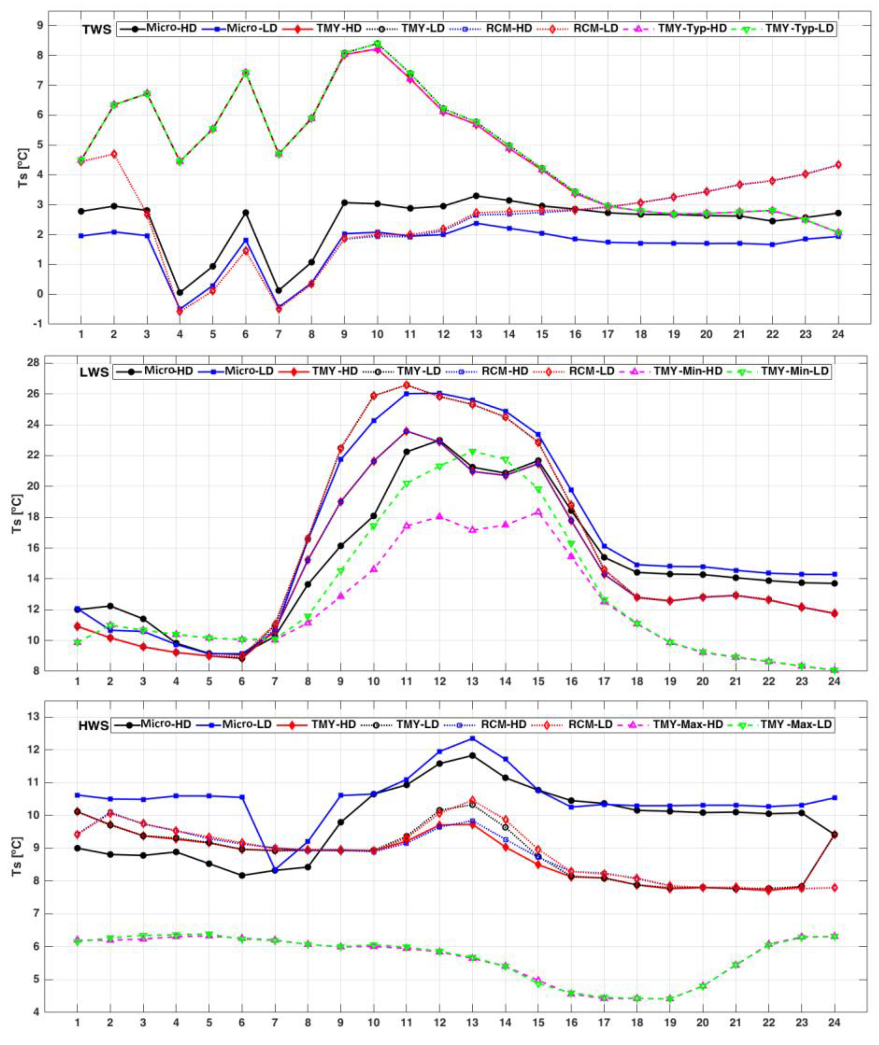
4.1. CFD Simulations
4.2. Energy Performance Simulations (EPS)
4.3. Limitations
5. Conclusions
Author Contributions
Funding
Conflicts of Interest
Nomenclature
| BPS | Building performance simulation | HD | High density |
| BMC | Building Modular Cells | LD | Low density |
| CC | cloud coverage | LWS | low wind speed |
| CFD | computational fluid dynamic | RCM | regional climate model |
| TMY | EnergyPlus Weather file | RH | Relative humidity |
| ED | Energy demand | TWS | Typical wind speed |
| GR | global radiation | T | Temperature [°C] |
| HWS | high wind speed | Surface temperature |
Appendix A

| Variables | Description | Value | Unit | |
|---|---|---|---|---|
| Loads | People | 0.2 | p/m2 | |
| Schedule behavior | As a simple office | |||
| Equipment | 12 | w/m2 | ||
| Schedule behavior | As a simple office | |||
| Lights | 12 | w/m2 | ||
| Illumination | 500 | lux | ||
| Dimming | continuous | - | ||
| Schedule behavior | As a simple office | - | ||
| Conditioning | Heating (Set point: 20) | 100 | w/m2 | |
| Cooling (Set points: 25) | 100 | w/m2 | ||
| Humidity control | No | - | ||
| Fresh air | 2.5 | L/s/person | ||
| Fresh air | 0.3 | L/s/zone area m2 | ||
| Sensible recovery ratio | 0.7 | - | ||
| Heat recovery | None | - | ||
| Scheduled | None | - | ||
| Buoyancy driven flow | 18–30 | C | ||
| Rel. Humidity | 80% | - | ||
| ACH | 0.2 | - | ||
| Hot water | Peak flow | 0.03 | m3/h/m2 | |
| Supply Temp | 65 | C | ||
| Main Temp | 10 | C | ||
| Schedule behavior | As a simple office | - | ||
| Construction | External walls | Reinforced concrete, plaster, insulation, mortar, composite facade | U = 0.4 polystyrene insulation according to NBC 19 Iran | W/m2K |
| Internal walls | Bricks, plaster, plaster | U = 0.7 No insulation | W/m2K | |
| Roof | Reinforced concrete, plaster, insulation, cement mosaic | U = 0.30 polystyrene insulation according to NBC 19 Iran | W/m2K | |
| Frame | Stainless steel | U = 0.9 | W/m2K | |
| Glass | Low-E | U = 1.70 (0.30) | W/m2K | |
| SHGC | 0.2 | - | ||
| Shading | None | - | ||
| Projection Factor | 50% | - | ||
| Glazing | North facade | 25% | 9* (2*2) win | |
| South façade | 15% | 5* (2*2) win | ||
| West façade | 8% | 3* (2*2) win | ||
| East façade | 8% | 3* (2*2) win | ||
References
- Brockerhoff, M.; Nations, U. World Urbanization Prospects: The 2018 Revision. Popul. Dev. Rev. 2018, 24, 883. [Google Scholar] [CrossRef]
- United Nations Population Division, Department of Economic and Social Affairs. The Worlds Cities in 2018 Data Booklet; United Nations Population Division, Department of Economic and Social Affairs: New York, NY, USA, 2018. [Google Scholar]
- IPCC. Climate Change 2014: Mitigation of Climate Change. Contribution of Working Group III to the Fifth Assessment Report of the Intergovernmental Panel on Climate Change; Edenhofer, O., Pichs-Madruga, R., Sokona, Y., Farahani, E., Kadner, S., Seyboth, K., Adler, A., Baum, I., Brunner, S., Eickemeier, P., et al., Eds.; Cambridge University Press: Cambridge, UK; New York, NY, USA, 2014. [Google Scholar]
- Mahdavinejad, M.; Javanroodi, K. Natural ventilation performance of ancient wind catchers, an experimental and analytical study-case studies: One-sided, two-sided and four-sided wind catchers. Int. J. Energy Technol. Policy 2014, 10, 36. [Google Scholar] [CrossRef]
- Antoniadou, P.; Papadopoulos, A.M. Occupants’ thermal comfort: State of the art and the prospects of personalized assessment in office buildings. Energy Build. 2017, 153, 136–149. [Google Scholar] [CrossRef]
- Griego, D.; Krarti, M.; Hernandez-Guerrero, A. Energy efficiency optimization of new and existing office buildings in Guanajuato, Mexico. Sustain. Cities Soc. 2015, 17, 132–140. [Google Scholar] [CrossRef]
- Kubilay, A.; Derome, D.; Carmeliet, J. Coupling of physical phenomena in urban microclimate: A model integrating air flow, wind-driven rain, radiation and transport in building materials. Urban Clim. 2018, 24, 398–418. [Google Scholar] [CrossRef]
- Hosham, A.F.; Kubota, T. Effects of Building Microclimate on the Thermal Environment of Traditional Japanese Houses during Hot-Humid Summer. Buildings 2019, 9, 22. [Google Scholar] [CrossRef]
- Paramita, B.; Fukuda, H.; Perdana Khidmat, R.; Matzarakis, A. Building Configuration of Low-Cost Apartments in Bandung—Its Contribution to the Microclimate and Outdoor Thermal Comfort. Buildings 2018, 8, 123. [Google Scholar] [CrossRef]
- Lai, D.; Liu, W.; Gan, T.; Liu, K.; Chen, Q. A review of mitigating strategies to improve the thermal environment and thermal comfort in urban outdoor spaces. Sci. Total Environ. 2019, 661, 337–353. [Google Scholar] [CrossRef]
- Dernie, D.; Gaspari, J. Building Envelope Over-Cladding: Impact on Energy Balance and Microclimate. Buildings 2015, 5, 715–735. [Google Scholar] [CrossRef]
- Zinzi, M.; Carnielo, E.; Mattoni, B. On the relation between urban climate and energy performance of buildings. A three-years experience in Rome, Italy. Appl. Energy 2018, 221, 148–160. [Google Scholar] [CrossRef]
- Oke, T.R.; Mills, G.; Christen, A.; Voogt, J.A. Urban Climates; Cambridge University Press: Cambridge, UK, 2017. [Google Scholar] [CrossRef]
- Li, H.; Zhou, Y.; Wang, X.; Zhou, X.; Zhang, H.; Sodoudi, S. Quantifying urban heat island intensity and its physical mechanism using WRF/UCM. Sci. Total Environ. 2019, 650, 3110–3119. [Google Scholar] [CrossRef] [PubMed]
- Janjai, S.; Deeyai, P. Comparison of methods for generating typical meteorological year using meteorological data from a tropical environment. Appl. Energy 2009, 86, 528–537. [Google Scholar] [CrossRef]
- Moazami, A.; Nik, V.M.; Carlucci, S.; Geving, S. Impacts of future weather data typology on building energy performance—Investigating long-term patterns of climate change and extreme weather conditions. Appl. Energy 2019, 238, 696–720. [Google Scholar] [CrossRef]
- Wyszogrodzki, A.A.; Miao, S.; Chen, F. Evaluation of the coupling between mesoscale-WRF and LES-EULAG models for simulating fine-scale urban dispersion. Atmos. Res. 2012, 118, 324–345. [Google Scholar] [CrossRef]
- Golden, J.S.; Kaloush, K.E. Mesoscale and microscale evaluation of surface pavement impacts on the urban heat island effects. Int. J. Pavement Eng. 2006, 7, 37–52. [Google Scholar] [CrossRef]
- Kondo, H.; Tokairin, T.; Kikegawa, Y. Calculation of wind in a Tokyo urban area with a mesoscale model including a multi-layer urban canopy model. J. Wind Eng. Ind. Aerodyn. 2008, 96, 1655–1666. [Google Scholar] [CrossRef]
- Santiago, J.L.; Krayenhoff, E.S.; Martilli, A. Flow simulations for simplified urban configurations with microscale distributions of surface thermal forcing. Urban Clim. 2014, 9, 115–133. [Google Scholar] [CrossRef]
- Li, X.; Mitra, C.; Dong, L.; Yang, Q. Understanding land use change impacts on microclimate using Weather Research and Forecasting (WRF) model. Phys. Chem. Earth 2018, 103, 115–126. [Google Scholar] [CrossRef]
- Mauree, D.; Naboni, E.; Coccolo, S.; Perera, A.T.D.; Nik, V.M.; Scartezzini, J.-L. A review of assessment methods for the urban environment and its energy sustainability to guarantee climate adaptation of future cities. Renew. Sustain. Energy Rev. 2019, 112, 733–746. [Google Scholar] [CrossRef]
- Futcher, J.A.; Mills, G. The role of urban form as an energy management parameter. Energy Policy 2013, 53, 218–228. [Google Scholar] [CrossRef]
- Shimazaki, Y.; Yoshida, A.; Suzuki, R.; Kawabata, T.; Imai, D.; Kinoshita, S. Application of human thermal load into unsteady condition for improvement of outdoor thermal comfort. Build. Environ. 2011, 46, 1716–1724. [Google Scholar] [CrossRef]
- Alcazar, S.S.; Olivieri, F.; Neila, J. Green roofs: Experimental and analytical study of its potential for urban microclimate regulation in Mediterranean–continental climates. Urban Clim. 2016, 17, 304–317. [Google Scholar] [CrossRef]
- Athamena, K.; Sini, J.-F.; Rosant, J.-M.; Guilhot, J. Numerical coupling model to compute the microclimate parameters inside a street canyon: Part II: Experimental validation of air temperature and airflow. Sol. Energy 2018, 170, 470–485. [Google Scholar] [CrossRef]
- Toparlar, Y.; Blocken, B.; Vos, P.; van Heijst, G.J.F.; Janssen, W.D.; van Hooff, T.; Timmermanse, H.J.P.; Montazeria, H. CFD simulation and validation of urban microclimate: A case study for Bergpolder Zuid, Rotterdam. Build. Environ. 2015, 83, 79–90. [Google Scholar] [CrossRef]
- Tien, P.W.; Calautit, J.K. Numerical analysis of the wind and thermal comfort in courtyards “skycourts” in high rise buildings. J. Build. Eng. 2019, 24, 100735. [Google Scholar] [CrossRef]
- Toparlar, Y.; Blocken, B.; Maiheu, B.; van Heijst, G.J.F. A review on the CFD analysis of urban microclimate. Renew. Sustain. Energy Rev. 2017, 80, 1613–1640. [Google Scholar] [CrossRef]
- Perini, K.; Magliocco, A. Effects of vegetation, urban density, building height, and atmospheric conditions on local temperatures and thermal comfort. Urban For. Urban Green. 2014, 13, 495–506. [Google Scholar] [CrossRef]
- Hargreaves, A.; Cheng, V.; Deshmukh, S.; Leach, M.; Steemers, K. Forecasting how residential urban form affects the regional carbon savings and costs of retrofitting and decentralized energy supply. Appl. Energy 2017, 186, 549–561. [Google Scholar] [CrossRef]
- Ouketta, S.; Bouchahm, Y. Numerical evaluation of urban geometry’s control of wind movements in outdoor spaces during winter period. Case Mediterr. Clim. Renew. Energy 2020, 146, 1062–1069. [Google Scholar] [CrossRef]
- Chen, Y.; Hong, T.; Piette, M.A. Automatic generation and simulation of urban building energy models based on city datasets for city-scale building retrofit analysis. Appl. Energy 2017, 205, 323–335. [Google Scholar] [CrossRef]
- Chen, Y.; Hong, T.; Luo, X.; Hooper, B. Development of city buildings dataset for urban building energy modeling. Energy Build. 2019, 183, 252–265. [Google Scholar] [CrossRef]
- Botham-Myint, D.; Recktenwald, G.W.; Sailor, D.J. Thermal footprint effect of rooftop urban cooling strategies. Urban Clim. 2015, 14, 268–277. [Google Scholar] [CrossRef]
- Kantzioura, A.; Kosmopoulos, P.; Zoras, S. Urban surface temperature and microclimate measurements in Thessaloniki. Energy Build. 2012, 44, 63–72. [Google Scholar] [CrossRef]
- Zhang, J.; Xu, L.; Shabunko, V.; Tay, S.E.R.; Sun, H.; Lau, S.S.Y.; Reindl, T. Impact of urban block typology on building solar potential and energy use efficiency in tropical high-density city. Appl. Energy 2019, 240, 513–533. [Google Scholar] [CrossRef]
- Kikumoto, H.; Ooka, R.; Han, M.; Nakajima, K. Consistency of mean wind speed in pedestrian wind environment analyses: Mathematical consideration and a case study using large-eddy simulation. J. Wind Eng. Ind. Aerodyn. 2018, 173, 91–99. [Google Scholar] [CrossRef]
- Zhang, J.; Wu, L. The influence of population movements on the urban relative humidity of Beijing during the Chinese Spring Festival holiday. J. Clean. Prod. 2018, 170, 1508–1513. [Google Scholar] [CrossRef]
- Giridharan, R.; Emmanuel, R. The impact of urban compactness, comfort strategies and energy consumption on tropical urban heat island intensity: A review. Sustain. Cities Soc. 2018, 40, 677–687. [Google Scholar] [CrossRef]
- Braulio-Gonzalo, M.; Bovea, M.D.; Ruá, M.J.; Juan, P. A methodology for predicting the energy performance and indoor thermal comfort of residential stocks on the neighbourhood and city scales. A case study in Spain. J. Clean. Prod. 2016, 139, 646–665. [Google Scholar] [CrossRef]
- Trihamdani, R.A.; Lee, S.H.; Kubota, T.; Phuong, T.T. Configuration of Green Spaces for Urban Heat Island Mitigation and Future Building Energy Conservation in Hanoi Master Plan 2030. Buildings 2015, 5, 933–947. [Google Scholar] [CrossRef]
- Elghonaimy, I.; Mohammed, E.W. Urban Heat Islands in Bahrain: An Urban Perspective. Buildings 2019, 9, 96. [Google Scholar] [CrossRef]
- Khoshdel Nikkho, S.; Heidarinejad, M.; Liu, J.; Srebric, J. Quantifying the impact of urban wind sheltering on the building energy consumption. Appl. Therm. Eng. 2017, 116, 850–865. [Google Scholar] [CrossRef]
- Wang, B.; Cot, L.D.; Adolphe, L.; Geoffroy, S.; Sun, S. Cross indicator analysis between wind energy potential and urban morphology. Renew. Energy 2017, 113, 989–1006. [Google Scholar] [CrossRef]
- Allegrini, J.; Dorer, V.; Carmeliet, J. Influence of morphologies on the microclimate in urban neighbourhoods. J. Wind Eng. Ind. Aerodyn. 2015, 144, 108–117. [Google Scholar] [CrossRef]
- Mittal, H.; Sharma, A.; Gairola, A. A review on the study of urban wind at the pedestrian level around buildings. J. Build. Eng. 2018, 18, 154–163. [Google Scholar] [CrossRef]
- Shirzadi, M.; Naghashzadegan, M.; Mirzaei, P.A. Developing a framework for improvement of building thermal performance modeling under urban microclimate interactions. Sustain. Cities Soc. 2019, 44, 27–39. [Google Scholar] [CrossRef]
- Javanroodi, K.; Mahdavinejad, M.; Nik, V.M. Impacts of urban morphology on reducing cooling load and increasing ventilation potential in hot-arid climate. Appl. Energy 2018, 231, 714–746. [Google Scholar] [CrossRef]
- Nik, V.M. Making energy simulation easier for future climate—Synthesizing typical and extreme weather data sets out of regional climate models (RCMs). Appl. Energy 2016, 177, 204–226. [Google Scholar] [CrossRef]
- Nik, V.M. Application of typical and extreme weather data sets in the hygrothermal simulation of building components for future climate—A case study for a wooden frame wall. Energy Build. 2017, 154, 30–45. [Google Scholar] [CrossRef]
- Weather Data EnergyPlus. Available online: https://energyplus.net/weather (accessed on 24 June 2019).
- Al-Sallal, K.A.; Al-Rais, L. Outdoor airflow analysis and potential for passive cooling in the traditional urban context of Dubai. Renew. Energy 2011, 36, 2494–2501. [Google Scholar] [CrossRef]
- Javanroodi, K.; Nik, V.M.; Mahdavinejad, M. A novel design-based optimization framework for enhancing the energy efficiency of high-rise office buildings in urban areas. Sustain. Cities Soc. 2019, 49, 101597. [Google Scholar] [CrossRef]
- Solemma LLC. Available online: https://www.solemma.com/ (accessed on 25 June 2019).


| Wind Speed | Types | Date | Scale | Generated Weather Data | STDV | Min | Average | Max |
|---|---|---|---|---|---|---|---|---|
| Typical | TWS | 02.19 | Meso | (1) RCM–TWS | 0.37 | 9.91 | 10.61 | 11.06 |
| Micro | (2) Micro-TWS (LD) | 0.22 | 0.11 | 0.43 | 0.9 | |||
| (3) Micro-TWS (HD) | 0.2 | 0.08 | 0.39 | 0.8 | ||||
| Meso | (4) TMY–TWS | 2.62 | 1 | 4.58 | 8.2 | |||
| EPW-TYP | 09.14 | Meso | (5) TMY–TYP | 0.93 | 0.5 | 1.65 | 3.1 | |
| Extreme low | LWS | 10.04 | Meso | (6) RCM–LWS | 0.28 | 0.16 | 0.56 | 1.14 |
| Micro | (7) Micro-LWS (LD) | 0.26 | 7.6 | 8.12 | 8.33 | |||
| (8) Micro-LWS (HD) | 0.29 | 5.31 | 5.82 | 6.36 | ||||
| Meso | (9) TMY–LWS | 0.28 | 0.2 | 0.57 | 1.2 | |||
| EPW-Min | 11.17 | Meso | (10) TMY-Min | 0.2 | 0 | 0.25 | 0.5 | |
| Extreme high | HWS | 01.15 | Meso | (11) RCM–HWS | 0.48 | 12.21 | 13.14 | 14.02 |
| Micro | (12) Micro-HWS (LD) | 0.3 | 7.98 | 8.57 | 9.16 | |||
| (13) Micro-HWS (HD) | 0.2 | 6.45 | 6.95 | 7.29 | ||||
| Meso | (14) TMY–HWS | 0.45 | 12.2 | 13.53 | 14 | |||
| EPW-Max | 01.13 | Meso | (15) TMY-Max | 4.46 | 6.2 | 12.55 | 18 |
| Weather Condition at Microscale | Urban Area | RCM | TMY (Typ, Min and Max) | ||||
|---|---|---|---|---|---|---|---|
| ED | ED | ||||||
| TWS | LD | −2% | +22% | +1% | −18% | −61% | −4% |
| HD | −6% | +11% | +3% | −13% | −39% | −1% | |
| LWS | LD | −17% | +8% | +1% | −58% | +28% | +4% |
| HD | −21% | +6% | +1% | −50% | +26% | +4% | |
| HWS | LD | −10% | +19% | +2% | −15% | +87% | +2% |
| HD | −13% | +13% | +2% | −18% | +77% | +2% | |
© 2019 by the authors. Licensee MDPI, Basel, Switzerland. This article is an open access article distributed under the terms and conditions of the Creative Commons Attribution (CC BY) license (http://creativecommons.org/licenses/by/4.0/).
Share and Cite
Javanroodi, K.; Nik, V.M. Impacts of Microclimate Conditions on the Energy Performance of Buildings in Urban Areas. Buildings 2019, 9, 189. https://doi.org/10.3390/buildings9080189
Javanroodi K, Nik VM. Impacts of Microclimate Conditions on the Energy Performance of Buildings in Urban Areas. Buildings. 2019; 9(8):189. https://doi.org/10.3390/buildings9080189
Chicago/Turabian StyleJavanroodi, Kavan, and Vahid M. Nik. 2019. "Impacts of Microclimate Conditions on the Energy Performance of Buildings in Urban Areas" Buildings 9, no. 8: 189. https://doi.org/10.3390/buildings9080189
APA StyleJavanroodi, K., & Nik, V. M. (2019). Impacts of Microclimate Conditions on the Energy Performance of Buildings in Urban Areas. Buildings, 9(8), 189. https://doi.org/10.3390/buildings9080189