A New Analytical Prediction for Energy Responses of Hemi-Cylindrical Shells to Explosive Blast Load


Abstract
1. Introduction
2. Systems of Motion
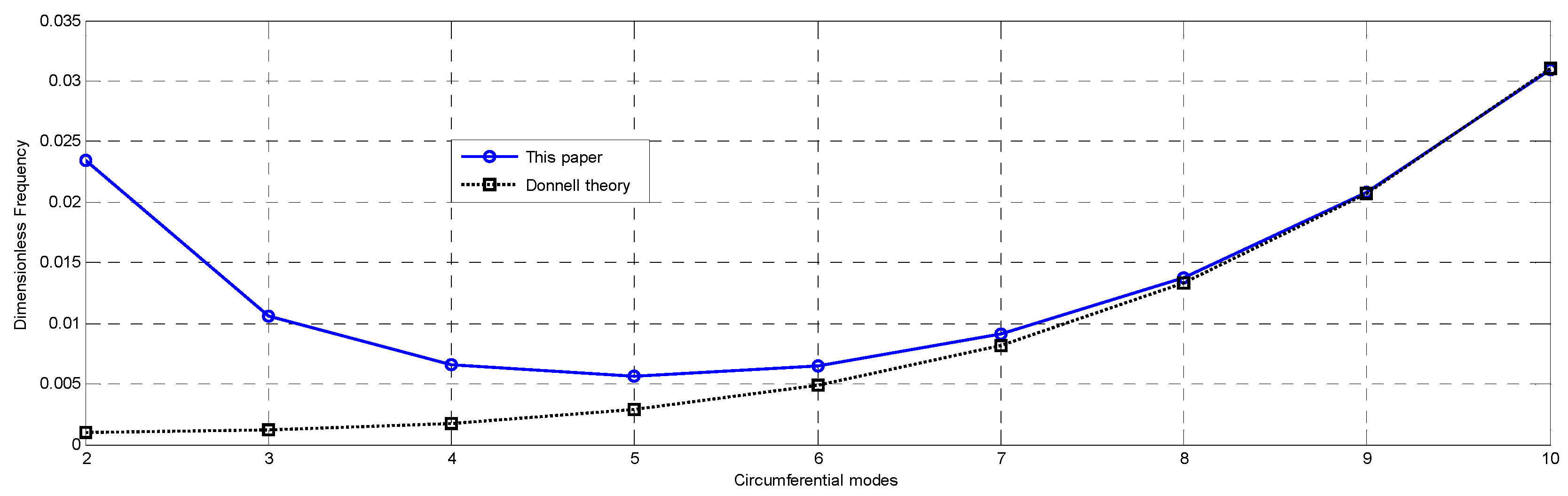
2.1. Frequency Analysis
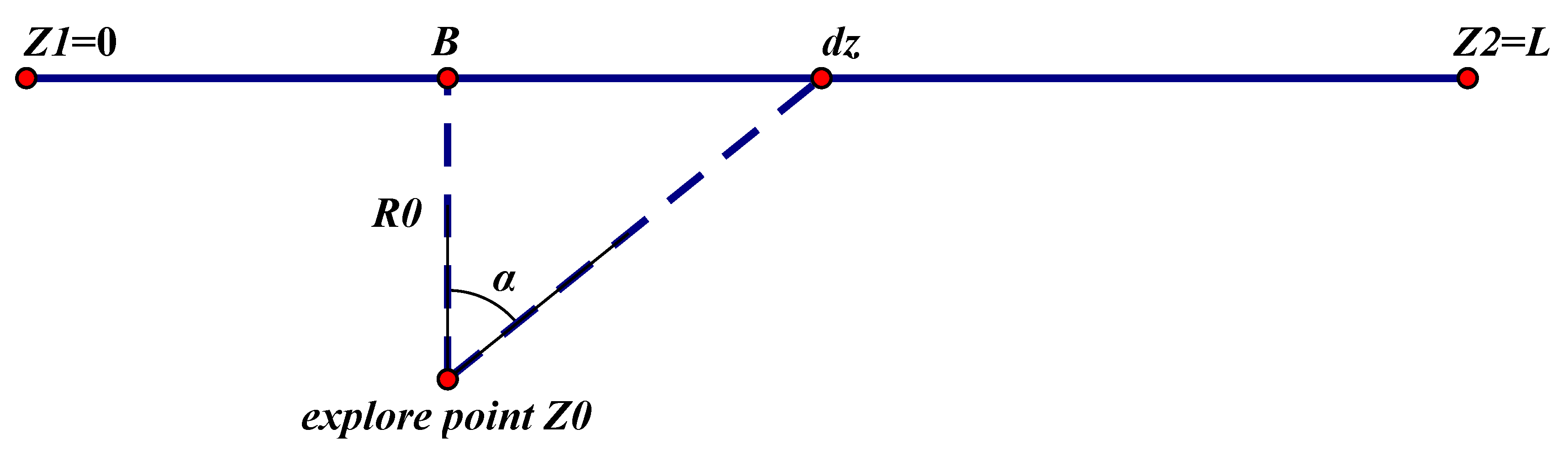
2.2. Relationship between Energy and Position
2.3. Energy Analysis of the Damping Load
2.4. Pressure Load
2.5. Numerical Verification
3. Numerical Simulations
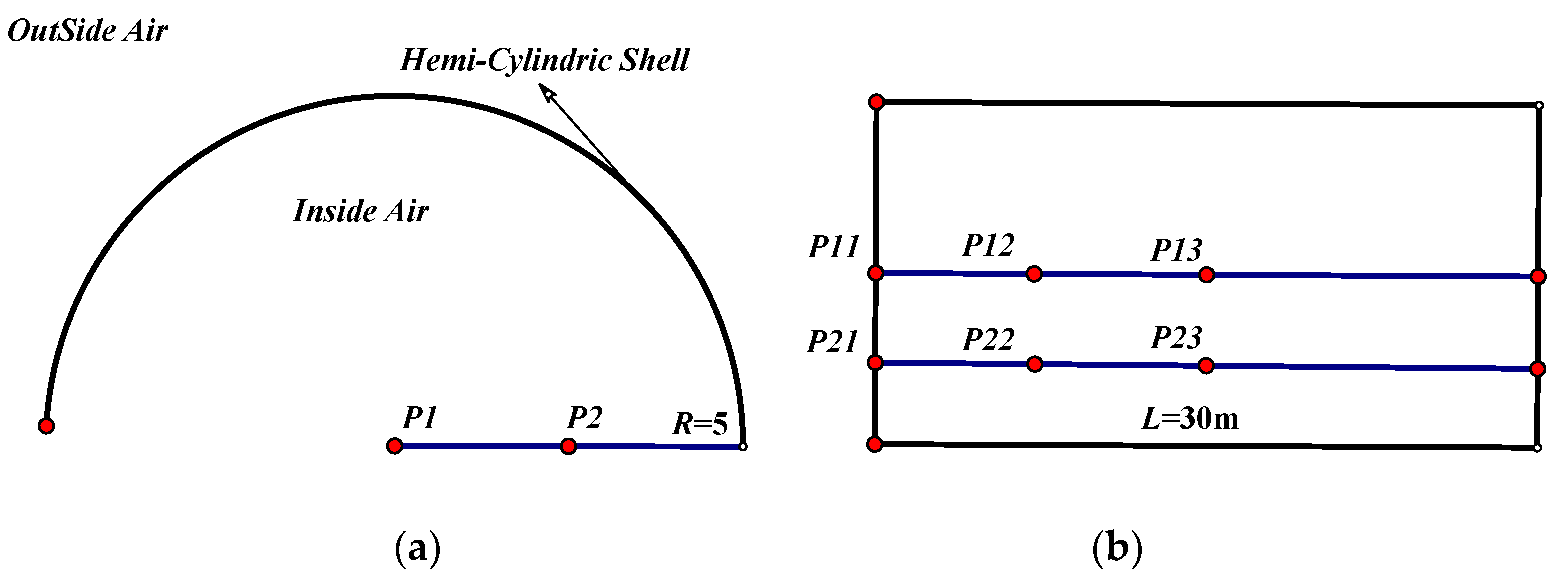
3.1. Simulation Model
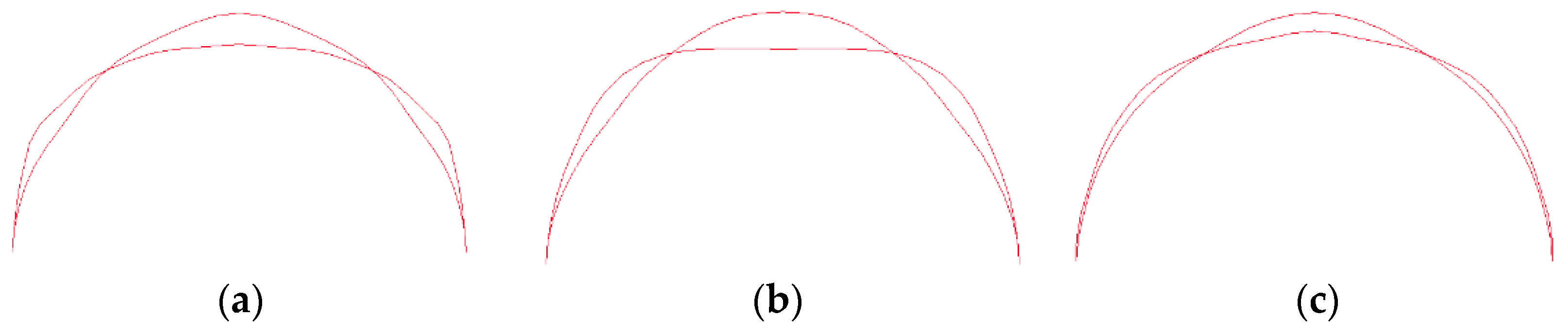
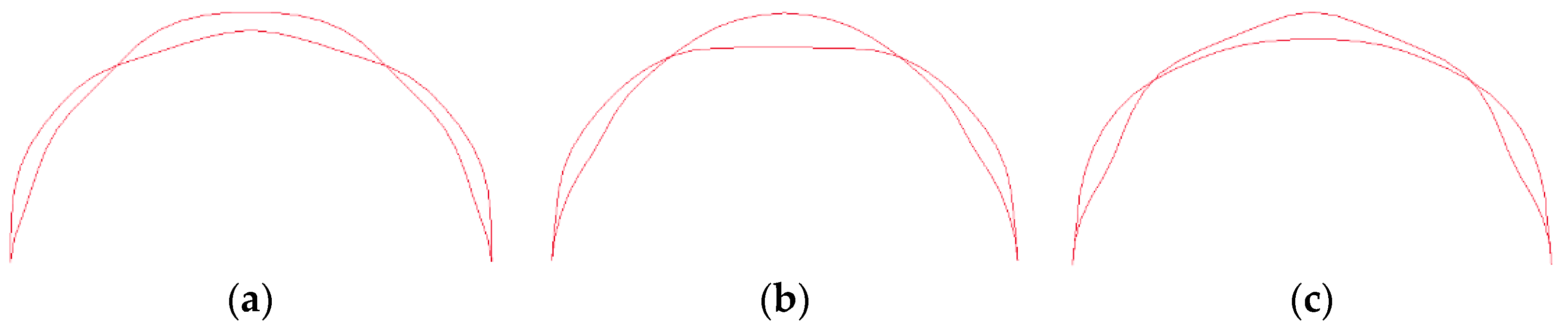
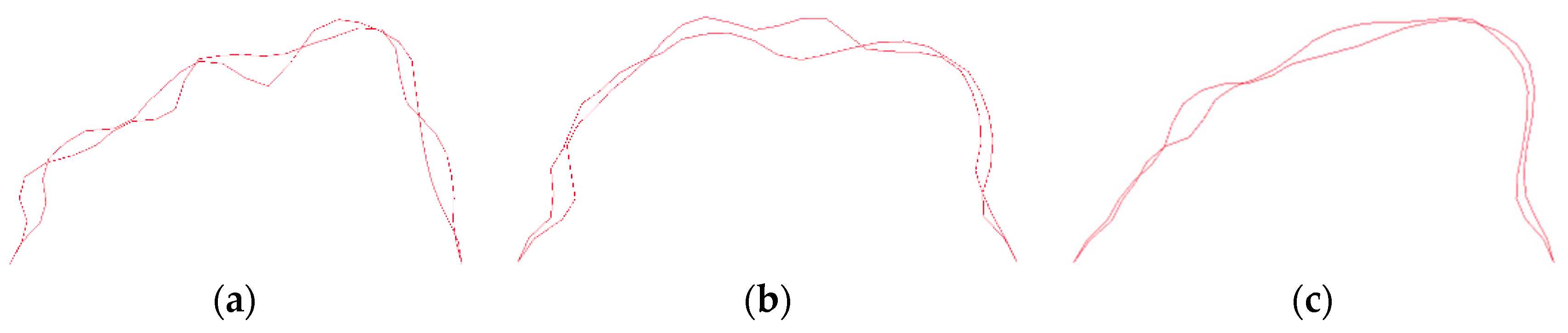
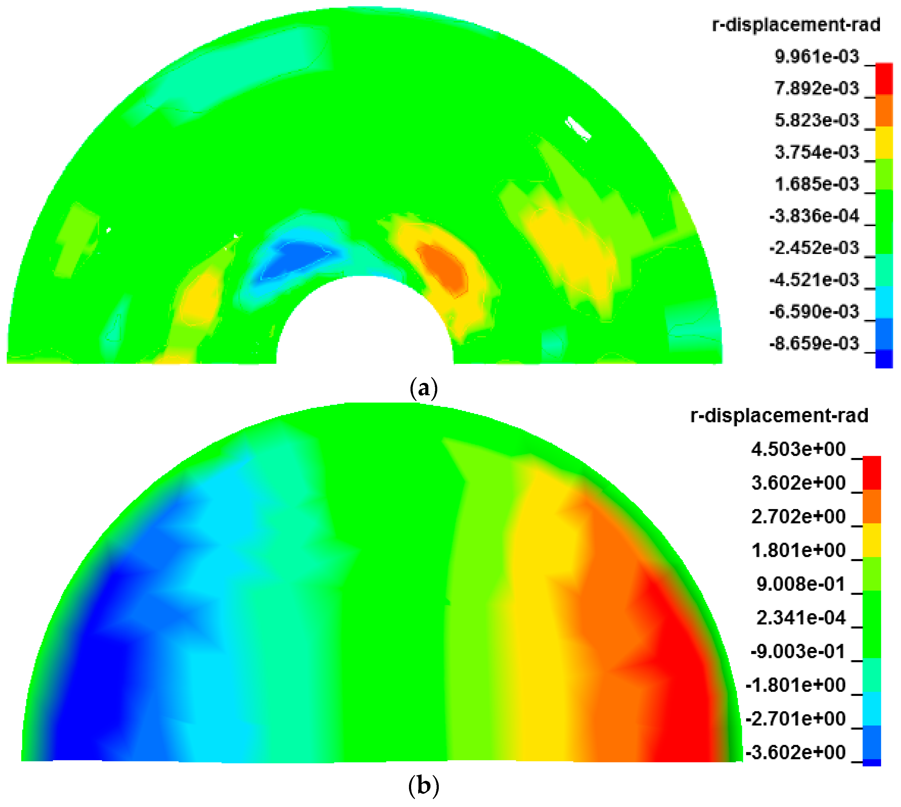
3.2. Natural Frequencies and Corresponding Mode Shapes
3.3. Global Energy
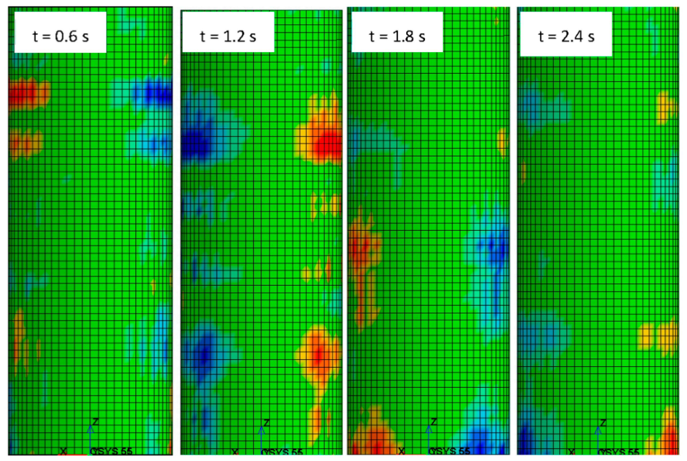
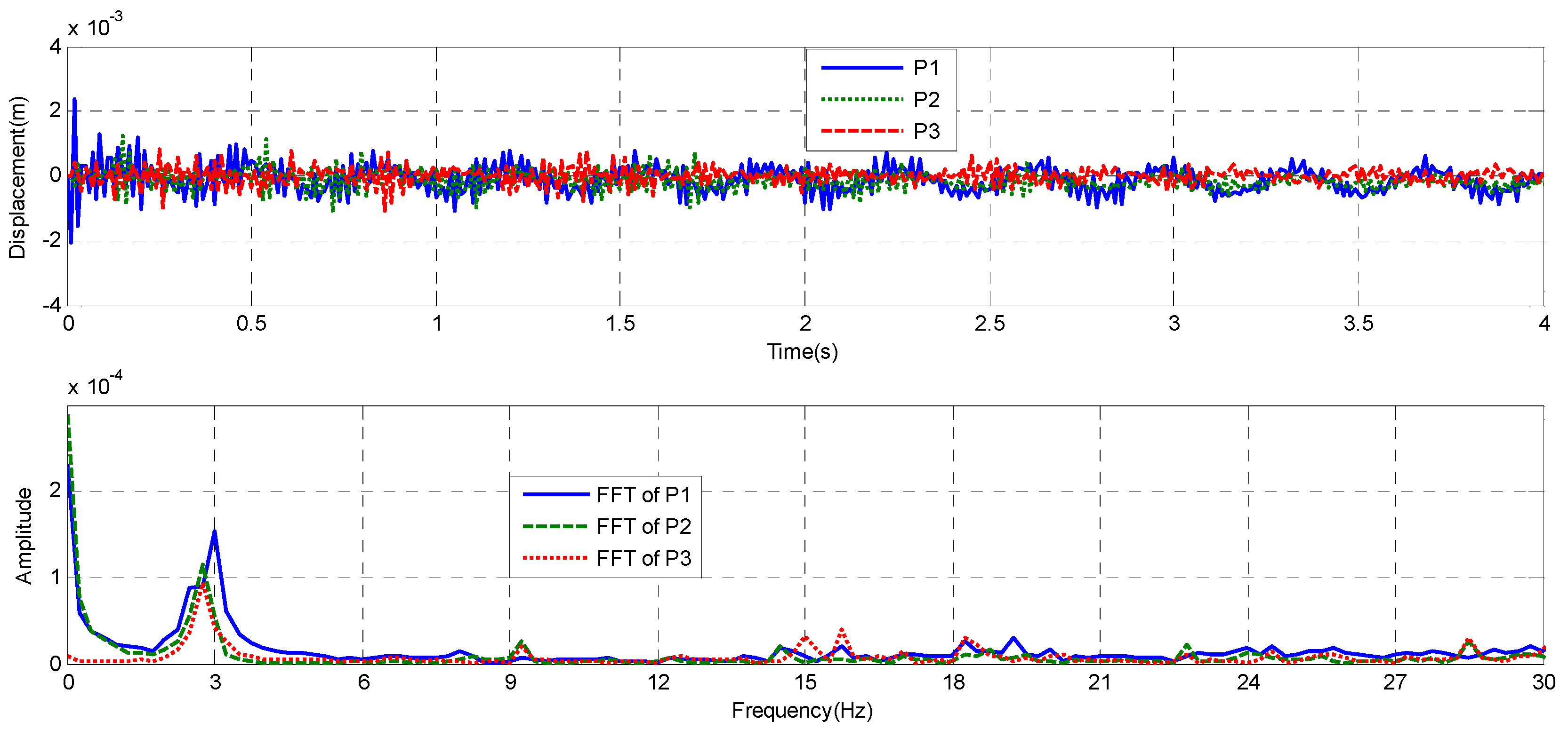
3.4. Displacement
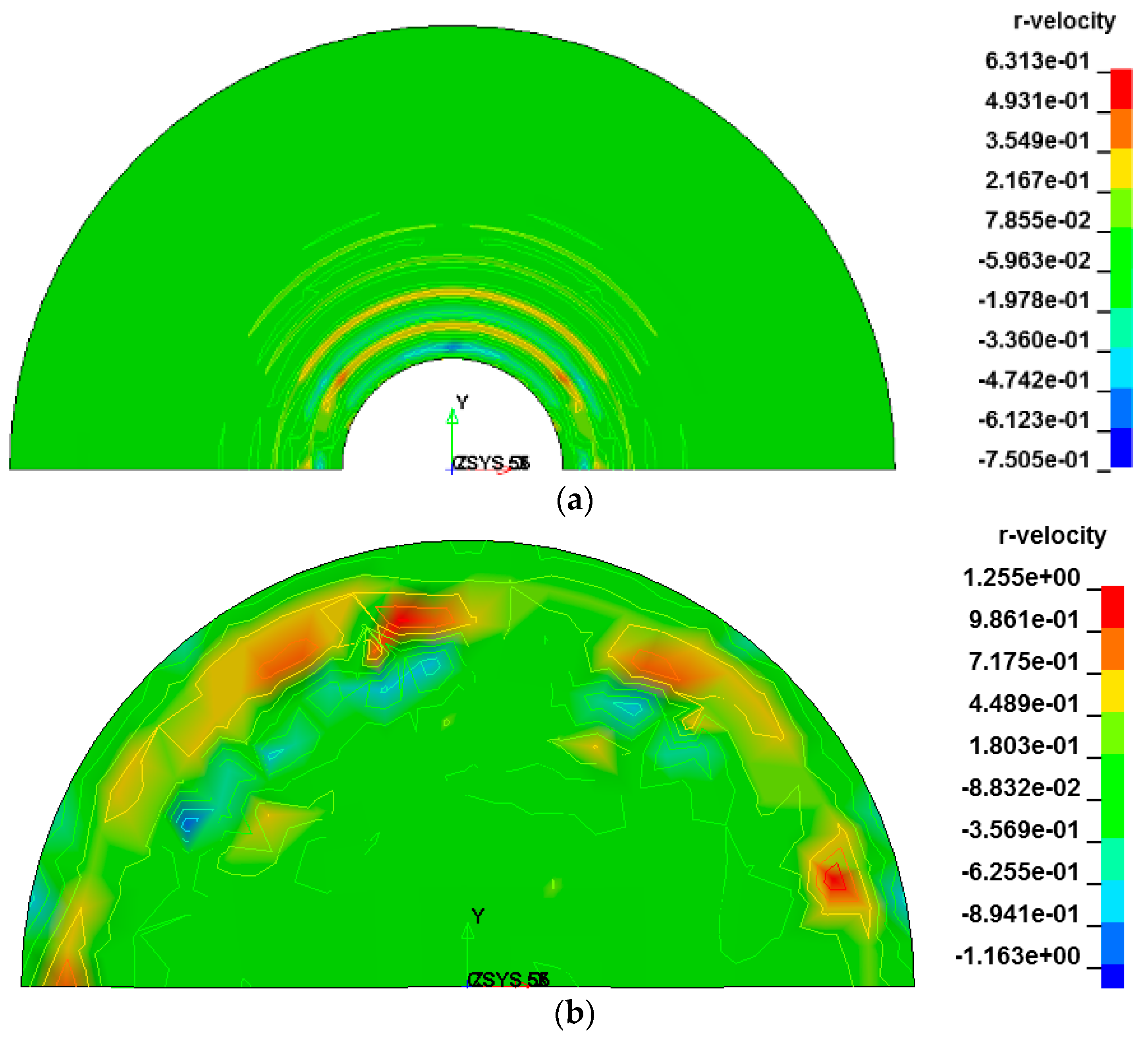
3.5. The Velocity of the Air Part
4. Parametric Analyses
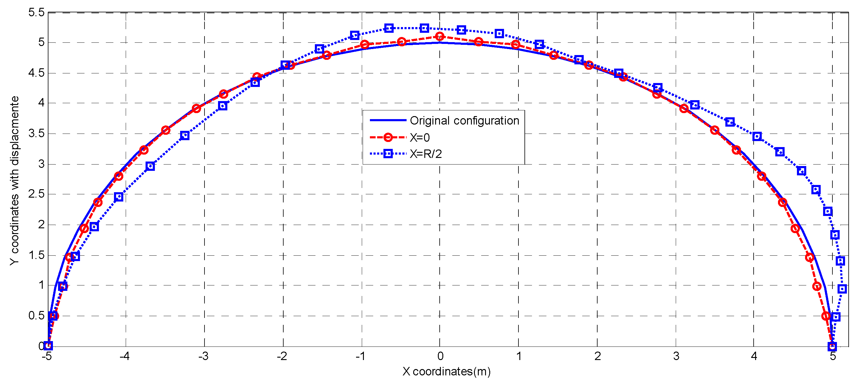
4.1. Displacement Analysis
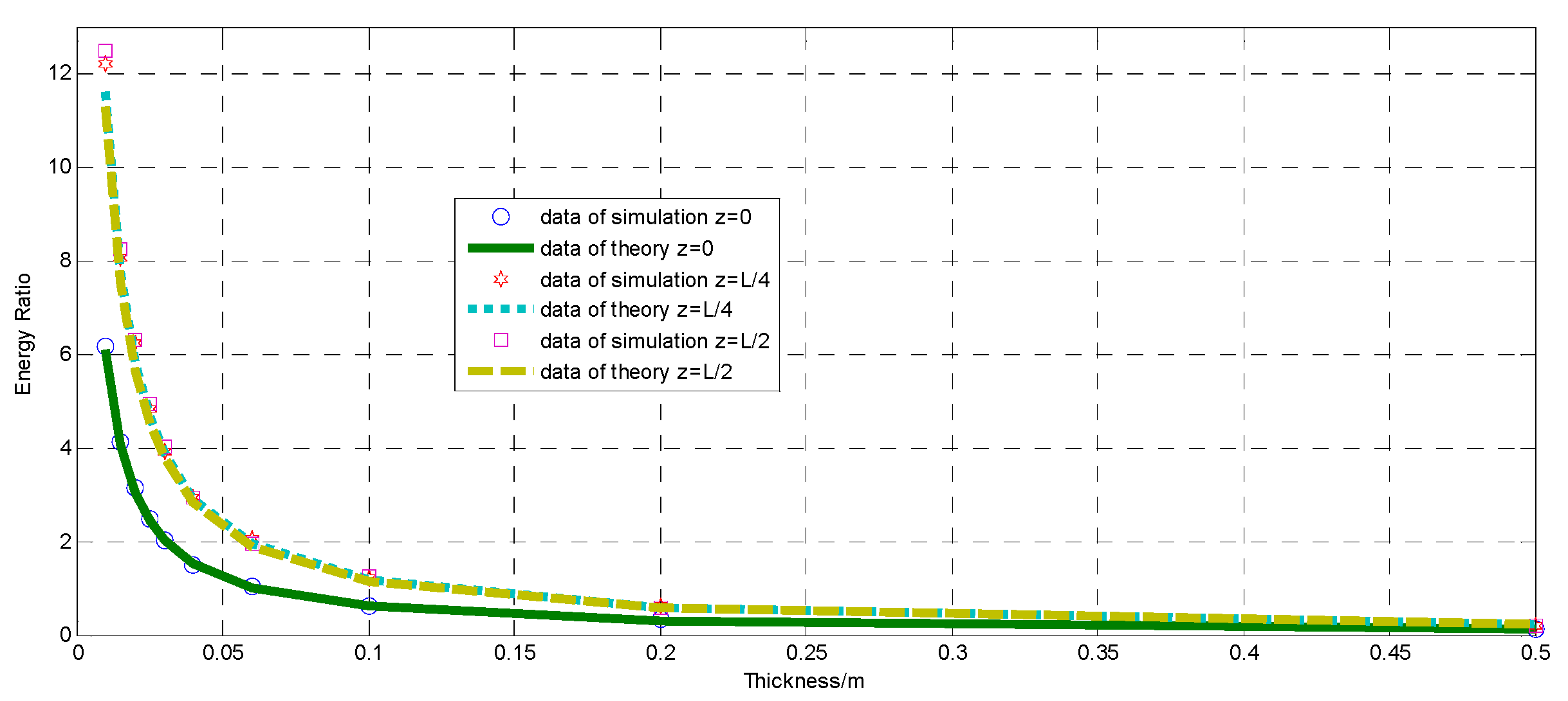
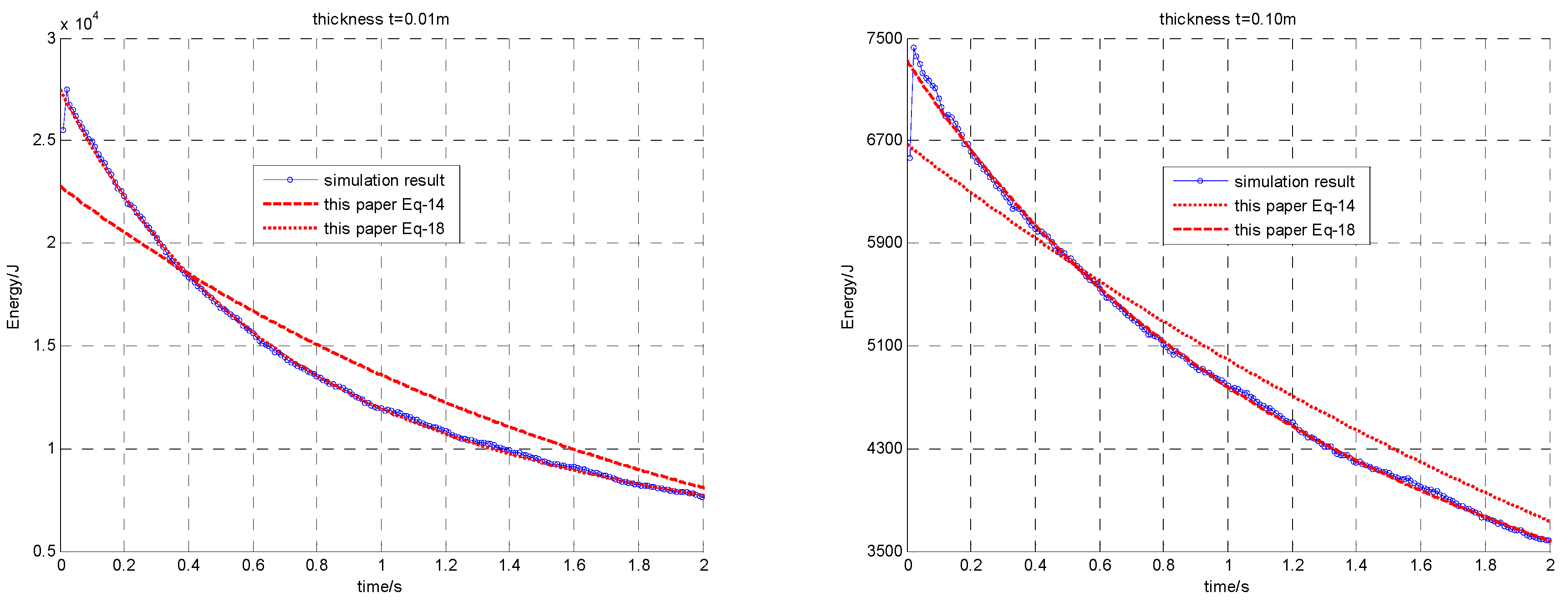
4.2. Total Energy vs. Thickness
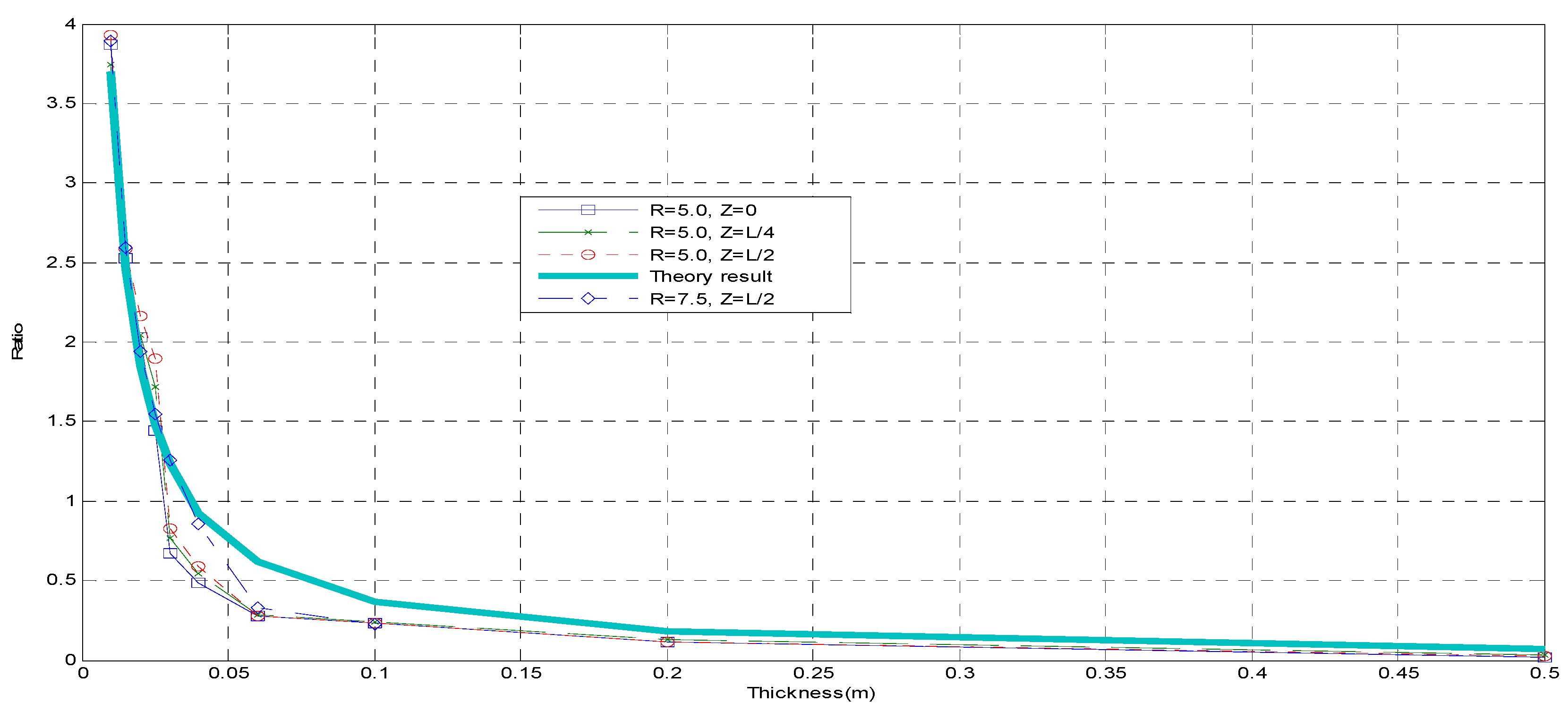
4.3. Decrease Ratio vs. Thickness
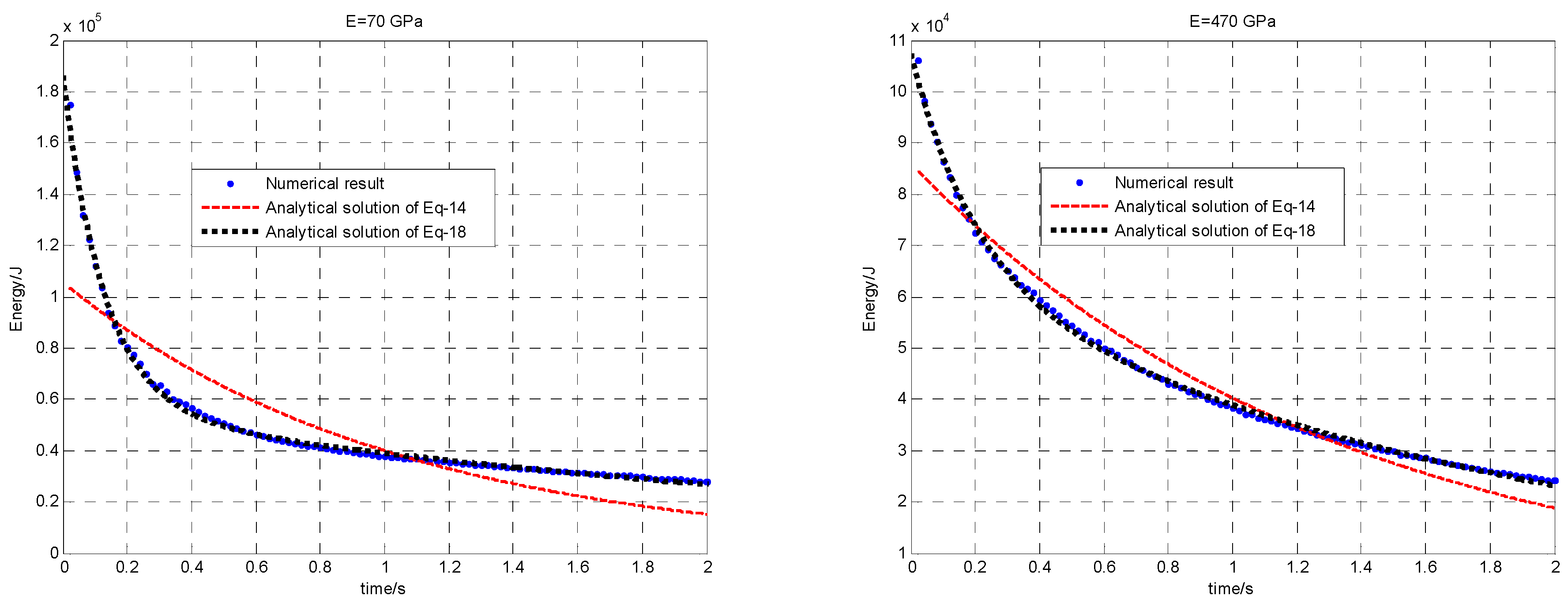
4.4. The Analysis of Elastic Modulus
4.5. Material Parameters
5. Conclusions
Author Contributions
Funding
Acknowledgments
Conflicts of Interest
References
- Liu, P.; Miu, W. Added Mass of Beam Vibration on Fluid with Finite Amplitude. In Proceedings of the International Conference on Civil, Structure, Environmental Engineering (I3CSEE 2016), Guang Zhou, China, 12–13 March 2016. [Google Scholar]
- Liu, P.; Kaewunruen, S.; Zhou, D.; Wang, S. Investigation of the Dynamic Buckling of Spherical Shell Structures Due to Subsea Collisions. Appl. Sci. 2018, 8, 1148. [Google Scholar] [CrossRef]
- Liu, P.; Kaewunruen, S.; Tang, B. Dynamic Pressure Analysis of Hemispherical Shell Vibrating in Unbounded Compressible Fluid. Appl. Sci. 2018, 8, 1938. [Google Scholar] [CrossRef]
- Zhang, J.; Zhang, M.; Cui, W.; Tang, W.; Wang, F.; Pan, B. Elastic-plastic buckling of deep sea spherical pressure hulls. Mar. Struct. 2018, 57, 38–51. [Google Scholar] [CrossRef]
- Zhang, J.; Wang, M.; Cui, W.; Wang, F.; Hua, Z.; Tang, W. Effect of thickness on the buckling strength of egg-shaped pressure hulls. Ships Offshore Struct. 2018, 13, 375–384. [Google Scholar] [CrossRef]
- Zhang, M.; Tang, W.; Wang, F.; Zhang, J.; Cui, W.; Chen, Y. Buckling of bi-segment spherical shells under hydrostatic external pressure. Thin-Walled Struct. 2017, 120, 1–8. [Google Scholar] [CrossRef]
- Sharma, P.K.; Patel, B.P.; Lal, H. On the Response of Hemispherical Shell under Blast Loading. Procedia Eng. 2017, 173, 533–538. [Google Scholar] [CrossRef]
- Agesh, M.; Lakshmana, R.C. Failure Analysis úof V-shaped Plates under Blast Loading. Procedia Eng. 2017, 173, 519–525. [Google Scholar]
- Ameijeiras, M.P.; Godoy, L.A. Simplified Analytical Approach to Evaluate the Nonlinear Dynamics of Elastic Cylindrical Shells Under Lateral Blast Loads. Lat. Am. J. Solids Struct. 2016, 13, 1281–1298. [Google Scholar] [CrossRef][Green Version]
- Hoo Fatt, M.S.; Sirivolu, D. Blast response of double curvature, composite sandwich shallow shells. Eng. Struct. 2015, 100, 696–706. [Google Scholar] [CrossRef]
- Li, W.; Huang, G.; Bai, Y.; Dong, Y.; Feng, S. Dynamic response of spherical sandwich shells with metallic foam core under external air blast loading-Numerical simulation. Compos. Struct. 2014, 116, 612–625. [Google Scholar] [CrossRef]
- Clubley, S.K. Long duration blast loading of cylindrical shell structures with variable fill level. Thin-Walled Struct. 2014, 85, 234–249. [Google Scholar] [CrossRef]
- Lawrence, V.; Kaewunruen, S.; Bartoli, G.; Baniotopoulos, C. CFD simulation of passenger hazard risk at railway station platforms due to explosive air blasts. In Proceedings of the 4th Thailand Rail Academic Symposium, Khao Yai, Pakchong, Nakhon Ratchasima, Thailand, 31 August–1 September 2017. [Google Scholar]
- Kaewunruen, S.; Pompeo, G.; Bartoli, G. Blast simulations and transient responses of longspan glass roof structures: A case of London’s railway station. In Proceedings of the 25th UKACM Conference on Computational Mechanics, Birmingham, UK, 12–13 April 2017. [Google Scholar]
- Clubley, S.K. Non-linear long duration blast loading of cylindrical shell structures. Eng. Struct. 2014, 59, 113–126. [Google Scholar] [CrossRef]
- Jiang, J.; Qlson, M.D. New design-analysis techniques for blast loaded stiffened box and cylindrical shell structures. Int. J. Impact Eng. 1993, 13, 189–202. [Google Scholar] [CrossRef]
- Saadin, B.; Leena, S.; Sakdirat, K.; Jaroszweski, D. Operational readiness for climate change of Malaysia high-speed rail. Proc. Inst. Civ. Eng. Transp 2016, 169, 308–320. [Google Scholar]
- Kaewunruen, S.; Yang, T.; Xu, S. Large amplitude free vibrations of spider web structures. In Proceedings of the 29th Nordic Seminar on Computational Mechanics, Gothenburg, Sweden, 26–28 October 2016. [Google Scholar]
- Zhai, X.; Wang, Y. Modelling and dynamic response of steel reticulated shell under blast loading. Shock Vib. 2013, 2013, 19–28. [Google Scholar] [CrossRef]
- Ebrahimi, M.J.; Najafizadeh, M.M. Free vibration analysis of two-dimensional functionally graded cylindrical shells. Appl. Math. Model. 2014, 38, 308–324. [Google Scholar] [CrossRef]
- Rahimi, G.H.; Ansari, R.; Hemmatnezhad, M. Vibration of functionally graded cylindrical shells with ring support. Sci. Iran. 2011, 18, 1313–1320. [Google Scholar] [CrossRef]
- Sirivolu, D.; Hoo Fatt, M.S. Dynamic stability of double-curvature composite shells under external blast. Int. J. Non-Linear Mech. 2015, 77, 281–290. [Google Scholar] [CrossRef]
- Pehrson, G.R.; Bannister, K.A. Airblast Loading Model for DYNA2D and DYNA3D. Army Res. Lab. 1997. [Google Scholar]
- Bibiana Luccionia, G.A. Erosioin Criteria for Frictional Materials under Blast Load. Mec. Comput. 2011, 39, 1809–1831. [Google Scholar]
- Hrvoje Draganić, V.S. Blast loading on structures. Djelovanje eksploz. Na Konstr. 2012, 19, 643–652. [Google Scholar]
- Turkmen, H.S. Structureal response of laminated composite shells subjected to blast loading: Comparison of experimental and theoretical methods. J. Sound Vib. 2002, 249, 663–678. [Google Scholar] [CrossRef]
- Santosa, S.P.; Arifurrahman, F.; Izzudin, M.H.; Widagdo, D.; Gunawan, L. Response Analysis of Blast Impact Loading of Metal-foam Sandwich Panels. Procedia Eng. 2017, 173, 495–502. [Google Scholar] [CrossRef]
- Wikipedia. Cylindrical Coordinate System [EB/OL]. Available online: https://en.wikipedia.org/wiki/Cylindrical_coordinate_system (accessed on 30 December 2017).
- Wikipedia. Kirchhoff–Love Plate Theory [EB/OL]. Available online: https://en.wikipedia.org/wiki/Kirchhoff/Love_plate_theory (accessed on 30 December 2016).
- Wikipedia. Vibration of Plates [EB/OL]. Available online: https://en.wikipedia.org/wiki/Vibration_of_plates (accessed on 30 December 2016).
- Tang, D.; WU, G.; YAO, X.; Wang, C. Free Vibration Analysis of Circular Cylindrical Shells with Arbitrary Boundary Conditions by the Method of Reverberation-Ray Matrix. Shock Vib. 2016, 2016, 1–18. [Google Scholar] [CrossRef]
- Chen, X.; Ye, K. Free Vibration Analysis for Shells of Revolution Using an Exact Dynamic Stiffness Method. Math. Probl. Eng. 2016, 2016, 1–12. [Google Scholar] [CrossRef]
- Putelat, T.; Triantafyllidis, N. Dynamic stability of externally pressurized elastic rings subjected to high rates of loading. Int. J. Solids Struct. 2014, 51, 1–12. [Google Scholar] [CrossRef]
- Johns, R.V.; Clubley, S.K. The influence of structural arrangement on long-duration blast response of annealed glazing. Int. J. Solids Struct. 2016, 97, 370–388. [Google Scholar] [CrossRef]
- Ma, J.L.; Wu, C.Q.; Zhi, X.D.; Fan, F. Prediction of Confined Blast Loading in Single-Layer Lattice Shells. Adv. Struct. Eng. 2014, 17, 1029–1043. [Google Scholar] [CrossRef]
- Kumari, E.; Singha, M.K. Nonlinear Response of Laminated Panels under Blast Load. Procedia Eng. 2017, 173, 539–546. [Google Scholar] [CrossRef]
- Caliri, M.F.; Ferreira, A.J.M.; Tita, V. A review on plate and shell theories for laminated and sandwich structures highlighting the Finite Element Method. Compos. Struct. 2016, 156, 63–77. [Google Scholar] [CrossRef]
- Kaewunruen, S.; Sussman, J.M.; Matsumoto, A. Grand Challenges in Transportation and Transit Systems. Front. Built Environ. 2016, 2, 4. [Google Scholar] [CrossRef]
- Kaewunruen, S. Underpinning systems thinking in railway engineering education. Australas. J. Eng. Educ. 2017, 22, 107–114. [Google Scholar] [CrossRef]
- Gorman, D.J.; Yu, S.D. A review of the superposition method for computing free vibration eigenvalues of elastic structures. Comput. Struct. 2012, 104, 27–37. [Google Scholar] [CrossRef]
- Qatu, M.S. Cylinderical Shells Vibration of Laminated Shells and Plates; ELsevier Academic Press: Cambridge, MA, USA, 2004; pp. 68–70. [Google Scholar]
- Schwer, L. Air Blast Reflection Ratios and Angle of Incidence. In Proceedings of the 11th European LS-DYNA Conference, Salzburg, Austria, 9–11 May 2017. [Google Scholar]
- Dewey, J.M. Measurement of the Physical Properties of Blast Waves. In Experimental Method of Shock Wave Research; Springer: Cham, Switzerland, 2016; Volume 33. [Google Scholar]
- Lawrence, V.; Ngamkhanong, C.; Kaewunruen, S. An Investigation to Optimize the Layout of Protective Blast Barriers Using Finite Element Modelling. Mater. Sci. Eng. 2017, 280, 375–383. [Google Scholar] [CrossRef]
- Vinson, J.R. The Vibration of Cylindrical Shells. In The Behavior of Thin Walled Structure: Beams, Plates and Shell; Kluwer Academic Publishers: Dordrecht, The Netherlands, 1989. [Google Scholar]
- On the Theory of Cylindrical Shells: Explicit Solution of the Characteristic Equation, and Discussion of the Accuracy of Various Shell Theories; IABSE Publications: New York, USA, 1953.
- Bajic, Z.; Bogdanov, J. Blast Effects Evaluation Using TNT Equivalent. Sci. Tech. Rev. 2009, 38, 50–57. [Google Scholar]
- Díaz Alonso, F.; González Ferradás, E.; Francisco Sánchez Pérez, J.; Aznar, A.M.; Gimeno, J.R.; Alonso, J.M. Characteristic overpressure–impulse–distance curves for the detonation of explosives, pyrotechnics or unstable substances. J. Loss Prev. Process Ind. 2006, 19, 724–728. [Google Scholar]
- Amiro, I.Y.; Prokopenko, N.Y. Study of nonlinear vibration of cylindrical shells with allowance for energy dissipatioin. Int. Appl. Mech. 1999, 35, 133–139. [Google Scholar] [CrossRef]
- Slavik, T.P. Blast Loading Todd in LS-DYNA; Livermore Software Technology Corporation: Troy, MI, USA, 2012. [Google Scholar]
- Brode, H.L. A Caculation of the Blast Wave for a Spherical Charge of TNT-1965; U.S. Air Force: Santa Monica, CA, USA, 1965.
- Chao, C.C.; Tung, T.P. Step pressure and blast responses of clamped orthotropic hemispherical shell. Int. J. Impact Eng. 1989, 8, 191–207. [Google Scholar] [CrossRef]
- Corporation, L.S.T. LS-DYNA® KEYWORD USER’S MANUAL I-VOLUMN 1; 7374 Las Positas Road Livermore, California 94551; Livermore Software Technology Corporation: Troy, MI, USA, 2017. [Google Scholar]
- Corporation, L.S.T. LS-DYNA® KEYWORD USER’S MANUAL II-Materials Model; 7374 Las Positas Road Livermore, California 94551; Livermore Software Technology Corporation: Troy, MI, USA, 2017. [Google Scholar]
- Jun, G.J. The experiment research on vibration characterisitcs of tensioned membrane structure. ShangXi Build. 2014, 19, 35–37. [Google Scholar]
- Gyliene, V.; Ostasevicius, V. Cowper-Symonds material deformation law application in material cutting process using LS-DYNA FE code: Turning and milling. In Proceedings of the 8th European LS-DYNA User’s Conference, Strasbourg, France, 19 May 2015. [Google Scholar]
- Lorenzo, B.; Marco, P.; Igiovanni, P. Identification of Strain-Rate Sensitivity Parameters of Steels With an Inverse Method. Exp. Anal. Nano Eng. Mater. Struct. 2007, 558, 291–294. [Google Scholar]
- Tan, K.T.; Huang, H.H.; Sun, C.T. Blast-wave impact mitigation using negative effective mass density concept of elastic metamaterials. Int. J. Impact Eng. 2014, 64, 20–29. [Google Scholar] [CrossRef]
- Yi, N.; Kim, J.J.; Han, T.; Cho, Y.G.; Lee, J.H. Blast-resistant characteristics of ultra-high strength concrete and reactive powder concrete. Constr. Build. Mater. 2011, 28, 694–707. [Google Scholar] [CrossRef]
- Katili, I.; Batoz, J.; Maknun, I.J.; Hamdouni, A.; Millet, O. The development of DKMQ plate bending element for thick to thin shell analysis based on the Naghdi/Reissner/Mindlin shell theory. Finite Elem. Anal. Des. 2015, 100, 12–27. [Google Scholar] [CrossRef]


| Density of Mesh (m) | 2.0 | 1.0 | 0.8 | 0.5 | 0.3 | 0.2 | 0.1 |
| Total Energy (104 J) | 4.52 | 4.21 | 3.93 | 3.90 | 3.89 | 3.89 | 3.88 |
| Max Displacement (mm) | 82 | 73 | 70 | 69 | 68 | 67 | 67 |
| 0.010 | 0/4 with x = 0 R = 5 L = 30 | 6.2 | 3.87 | 1/4 with x = 0 R = 5 L = 30 | 12 | 3.74 | 2/4 with x = 0 R = 5 L = 30 | 12.5 | 3.93 | 2/4 with x = 0 R = 7.5 L = 30 | 9.9 | 3.89 |
| 0.015 | 4.1 | 2.53 | 8.1 | 2.46 | 8.25 | 2.59 | 6.6 | 2.59 | ||||
| 0.020 | 3.2 | 2.03 | 6.2 | 2.04 | 6.31 | 2.16 | 4.9 | 1.94 | ||||
| 0.025 | 2.5 | 1.44 | 4.8 | 1.72 | 4.94 | 1.89 | 4.0 | 1.55 | ||||
| 0.030 | 2.0 | 0.87 | 3.9 | 0.77 | 4.03 | 0.83 | 3.3 | 1.26 | ||||
| 0.040 | 1.5 | 0.69 | 2.9 | 0.65 | 2.94 | 0.69 | 2.3 | 0.86 | ||||
| 0.060 | 1.0 | 0.38 | 2.0 | 0.39 | 1.96 | 0.38 | 1.5 | 0.33 | ||||
| 0.100 | 0.6 | 0.24 | 1.2 | 0.24 | 1.25 | 0.24 | 1.0 | 0.23 | ||||
| 0.200 | 0.3 | 0.12 | 0.6 | 0.13 | 0.59 | 0.12 | ||||||
| 0.500 | 0.1 | 0.02 | 0.2 | 0.03 | 0.19 | 0.03 |
| 0.010 | 0/4 with ×2.5 R = 5 | 5.2 | 1.6 | 5.12 | 0.38 | 1/4 with ×2.5 R = 5 | 9.8 | 3.6 | 4.46 | 0.32 | 2/4 with ×0.0 R = 7.5 | 9.9 | 3.89 |
| 0.015 | 3.2 | 1.4 | 3.35 | 0.26 | 5.9 | 3.4 | 3.57 | 0.28 | 6.6 | 2.59 | |||
| 0.020 | 2.0 | 1.5 | 2.95 | 0.32 | 4.1 | 3.0 | 3.01 | 0.25 | 4.9 | 1.94 | |||
| 0.025 | 1.6 | 1.2 | 1.74 | 0.24 | 3.1 | 2.5 | 1.81 | 0.24 | 4.0 | 1.55 | |||
| 0.030 | 0.8 | 1.5 | 1.30 | 0.37 | 2.4 | 2.4 | 1.86 | 0.27 | 3.3 | 1.26 | |||
| 0.040 | 0.8 | 0.9 | 1.24 | 0.15 | 1.6 | 1.9 | 1.41 | 0.17 | 2.3 | 0.86 | |||
| 0.060 | 0.6 | 0.6 | 1.07 | 0.13 | 1.3 | 1.1 | 1.18 | 0.13 | 1.5 | 0.33 | |||
| 0.100 | 0.3 | 0.5 | 1.11 | 0.17 | 0.6 | 0.9 | 1.07 | 0.16 | 1.0 | 0.23 |
| 910 | Case 1 0.23 Z = 0/4 × 0.0 | 1.89 | 3.29 | Case 2 0.13 Z = 0/4 × 0.0 | 1.91 | 3.28 | Case 3 0.07 Z = 2/4 × 2.5 | 3.37 | 3.25 | 5.28 | 0.30 |
| 470 | 3.46 | 3.45 | 3.52 | 3.45 | 2.11 | 5.09 | 3.53 | 0.61 | |||
| 210 | 6.16 | 3.82 | 5.91 | 3.86 | 10.8 | 6.41 | 3.73 | 0.55 | |||
| 170 | 6.76 | 4.01 | 7.26 | 3.95 | 12.7 | 7.19 | 3.10 | 0.46 | |||
| 140 | 7.81 | 4.29 | 8.25 | 4.53 | 12.2 | 7.34 | 4.40 | 0.52 | |||
| 70 | 10.2 | 4.55 | 11.7 | 4.62 | 13.0 | 7.82 | 5.65 | 0.37 | |||
| 40 | 11.8 | 4.29 | 11.7 | 4.42 | 11.5 | 9.13 | 6.78 | 0.31 | |||
| 10 | 14.3 | 4.31 | 13.8 | 4.37 | 8.64 | 14.6 | 19.7 | 0.05 |
| (ton/m3) | 10 | 7.8 | 4.0 | 2.0 | 1.0 | 0.6 | 0.3 |
| (104 J) | 1.94 | 2.13 | 2.31 | 2.31 | 2.18 | 1.95 | 1.80 |
| 4.62 | 3.84 | 2.18 | 1.16 | 1.73 | 2.33 | 3.53 |
| (ton/m3) | 10 | 7.8 | 4.0 | 2.0 | 1.0 |
| (104 J) | 5.62 | 6.08 | 7.52 | 7.86 | 8.21 |
| 4.63 | 3.76 | 3.12 | 1.48 | 2.75 | |
| / | / | 0.12 | 0.03 | 0.06 |
© 2019 by the authors. Licensee MDPI, Basel, Switzerland. This article is an open access article distributed under the terms and conditions of the Creative Commons Attribution (CC BY) license (http://creativecommons.org/licenses/by/4.0/).
Share and Cite
Liu, P.; Xu, N.; Pan, Z.-H. A New Analytical Prediction for Energy Responses of Hemi-Cylindrical Shells to Explosive Blast Load. Buildings 2019, 9, 168. https://doi.org/10.3390/buildings9070168
Liu P, Xu N, Pan Z-H. A New Analytical Prediction for Energy Responses of Hemi-Cylindrical Shells to Explosive Blast Load. Buildings. 2019; 9(7):168. https://doi.org/10.3390/buildings9070168
Chicago/Turabian StyleLiu, Ping, Ning Xu, and Zhi-Hong Pan. 2019. "A New Analytical Prediction for Energy Responses of Hemi-Cylindrical Shells to Explosive Blast Load" Buildings 9, no. 7: 168. https://doi.org/10.3390/buildings9070168
APA StyleLiu, P., Xu, N., & Pan, Z.-H. (2019). A New Analytical Prediction for Energy Responses of Hemi-Cylindrical Shells to Explosive Blast Load. Buildings, 9(7), 168. https://doi.org/10.3390/buildings9070168