Pushover-Based Seismic Capacity Evaluation of Uto City Hall Damaged by the 2016 Kumamoto Earthquake


Abstract
:1. Introduction
1.1. Background
1.2. Brief Review of Related Studies
1.3. Objectives
2. Seismic Capacity Evaluation Procedure
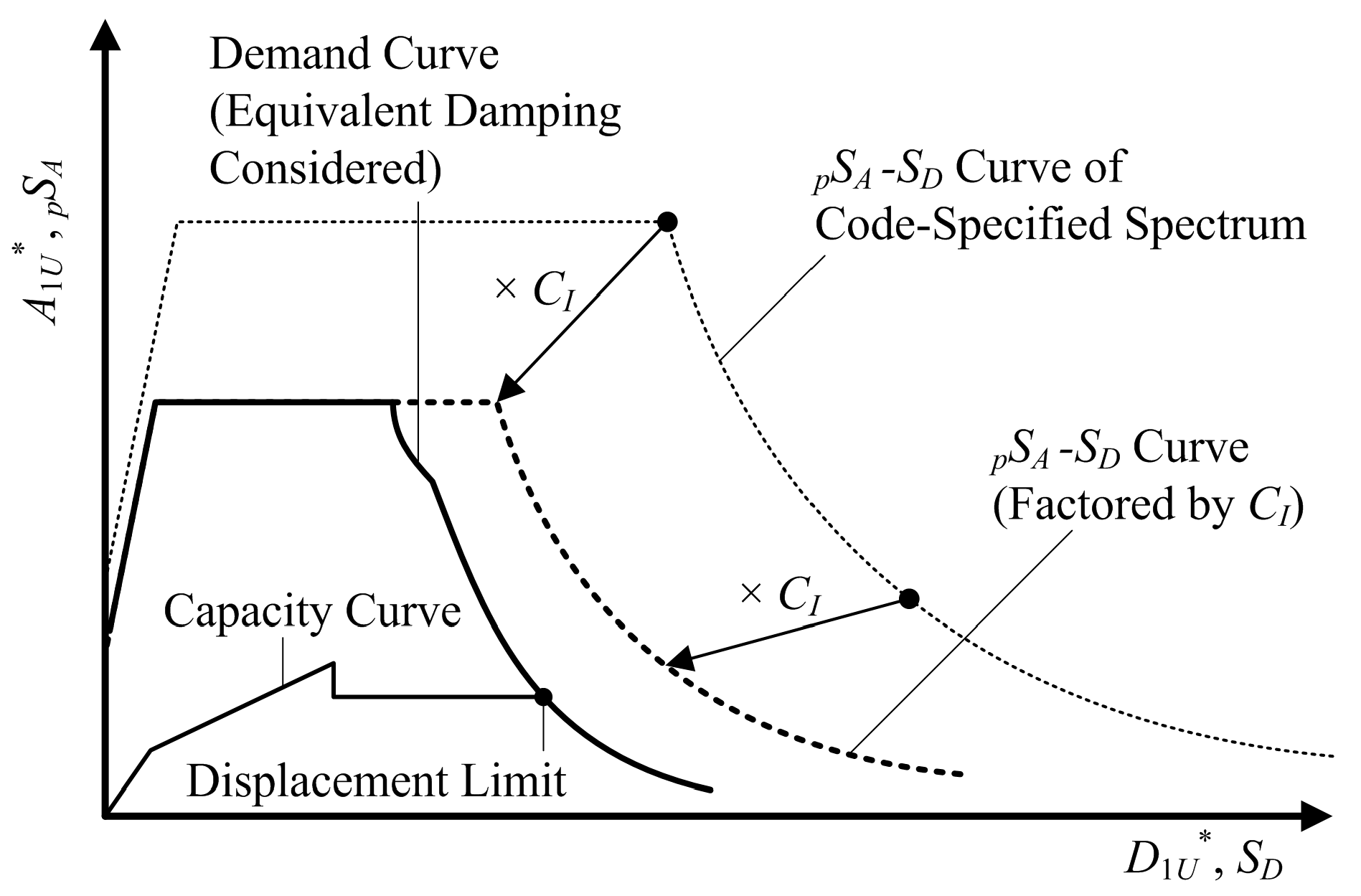
2.1. Definition of Seismic Capacity Index
2.2. Evaluation of the Seismic Capacity Index Considering the Unidirectional Ground Motion
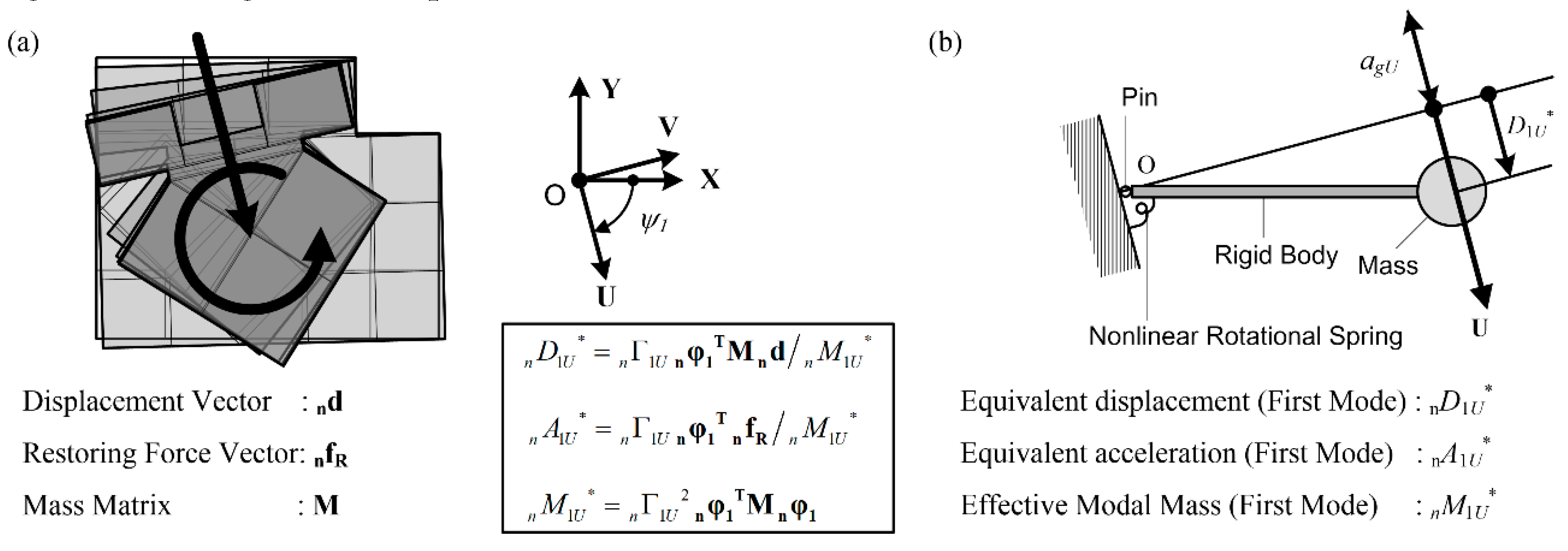
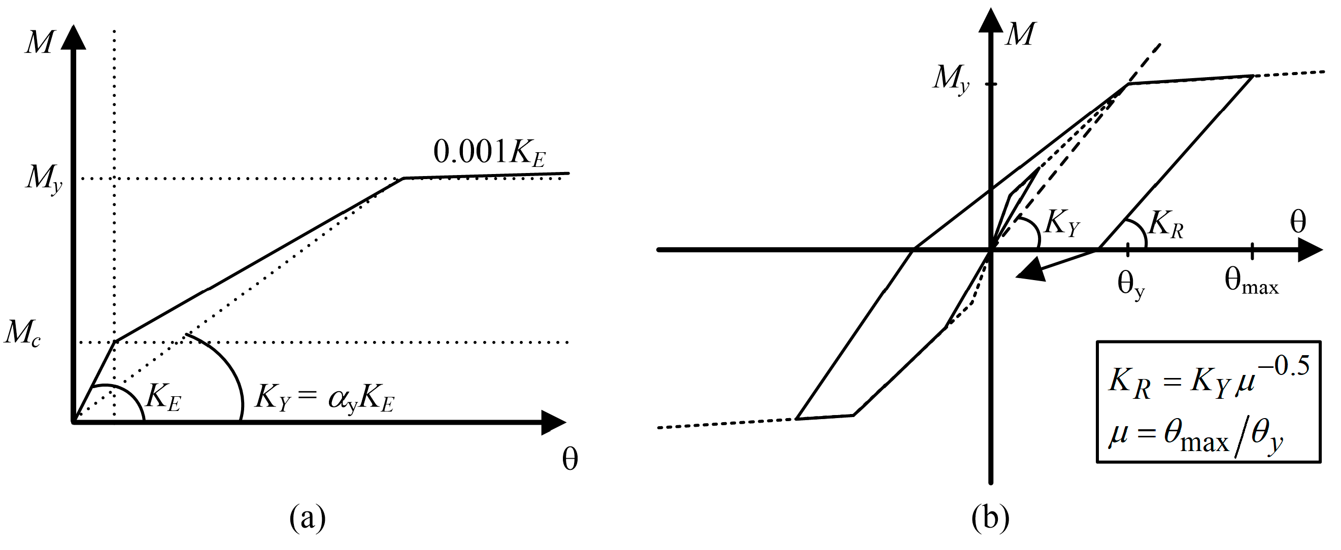
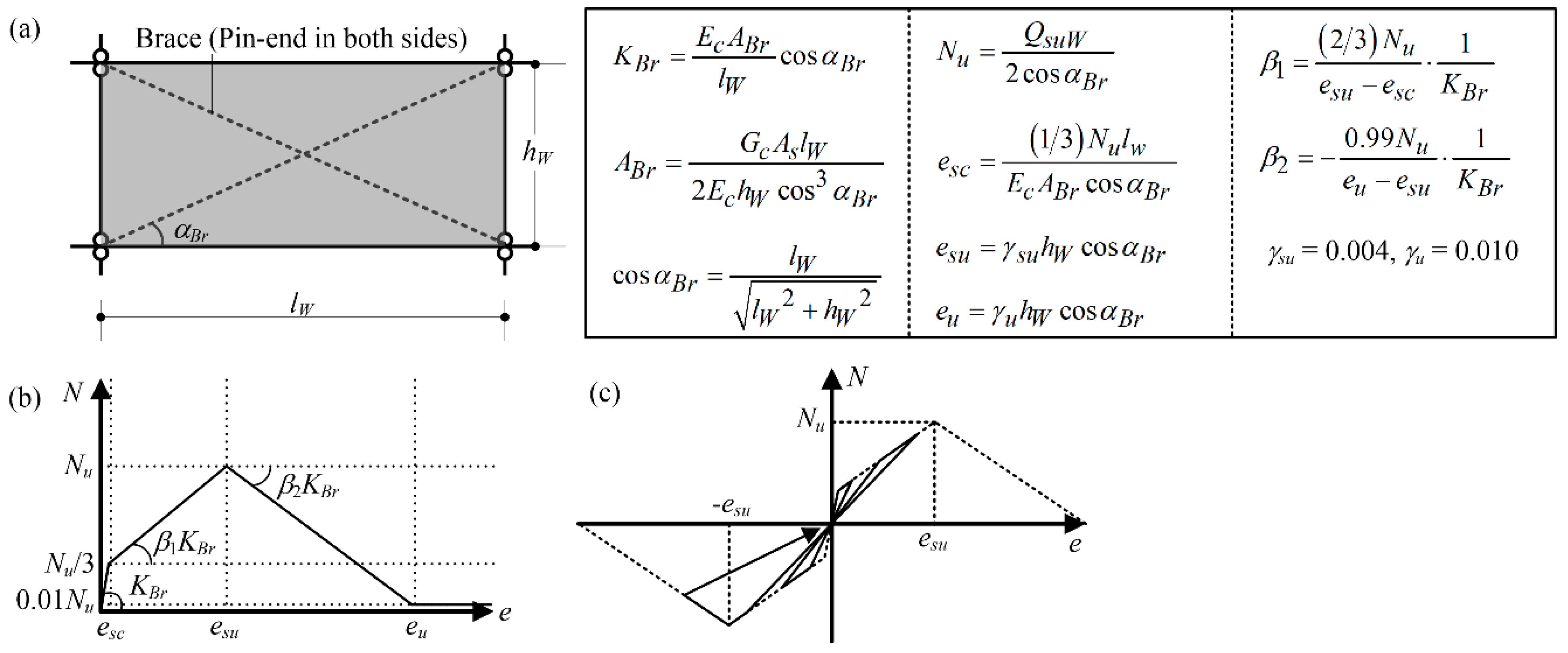
2.2.1. Step 1: Pushover Analysis of Building Model (First Mode)
- The envelope curve of the force-deformation relationship for each nonlinear spring of all members is symmetric in the positive and negative loading direction.
- The equivalent stiffness of each nonlinear spring can be defined by its secant stiffness at the peak deformation that was previously derived in the calculation.
- The first mode shape at each loading step () can be determined according to the equivalent stiffness.
- The displacement vector at each loading step (nd) imposed on the model is similar to the first mode shape obtained in assumptions 2 and 3.
- In the case where unloading occurs, the equivalent stiffness obtained in assumption 2 is used as the unloading stiffness for all nonlinear springs.
2.2.2. Step 2: Calculation of the Scaling Factor Corresponding to Each Pushover Step
2.2.3. Step 3: Evaluation of the Seismic Capacity Index
2.3. Evaluation of the Seismic Capacity Index Considering the Bidirectional Ground Motion
2.3.1. Steps 1 to 3: Evaluation of the Seismic Capacity Index Considering the Unidirectional Ground Motion
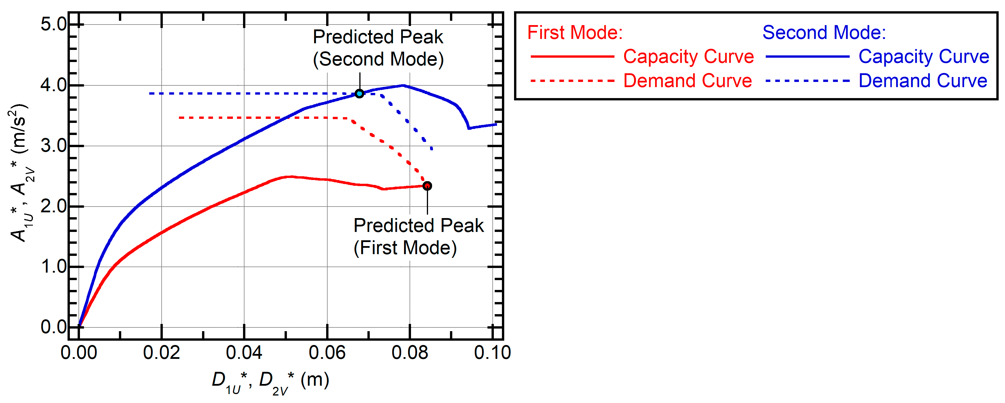
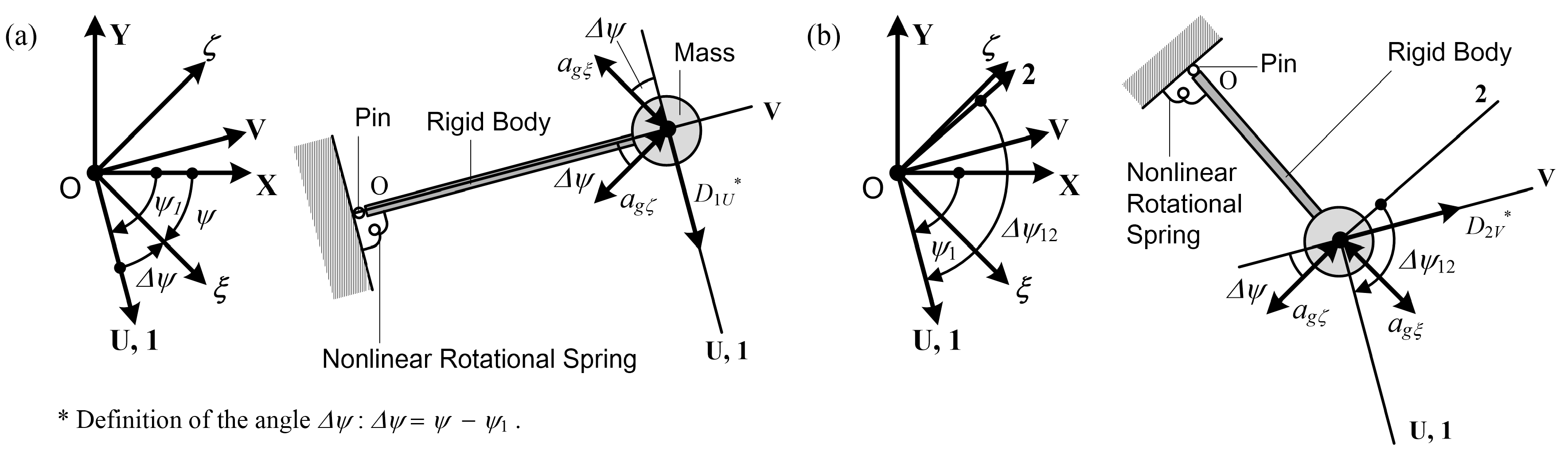
2.3.2. Step 4: Prediction of the Peak Response of the Equivalent SDOF Model (first mode)
2.3.3. Step 5: Pushover Analysis of the Building Model (second mode)
2.3.4. Step 6: Peak Response Prediction for the Equivalent SDOF Model (second mode)
2.3.5. Step 7: Pushover Analysis of the Building Model Considering the Bidirectional Seismic Input
2.3.6. Step 8: Evaluation of the Seismic Capacity Index Considering the Bidirectional Ground Motion
3. Building and Ground Motion Data
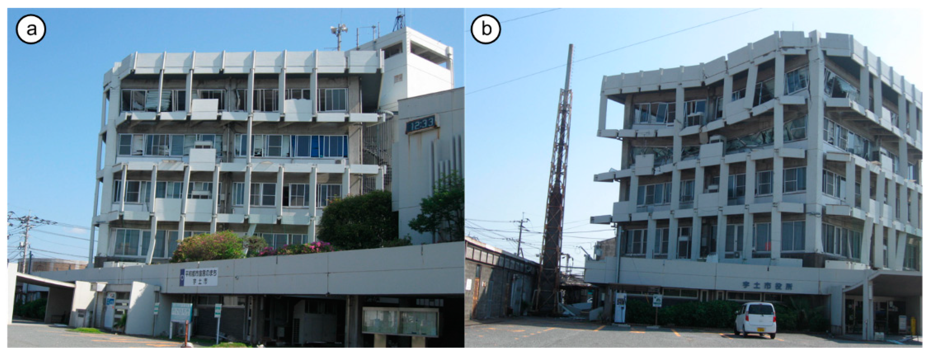
3.1. Basic Information
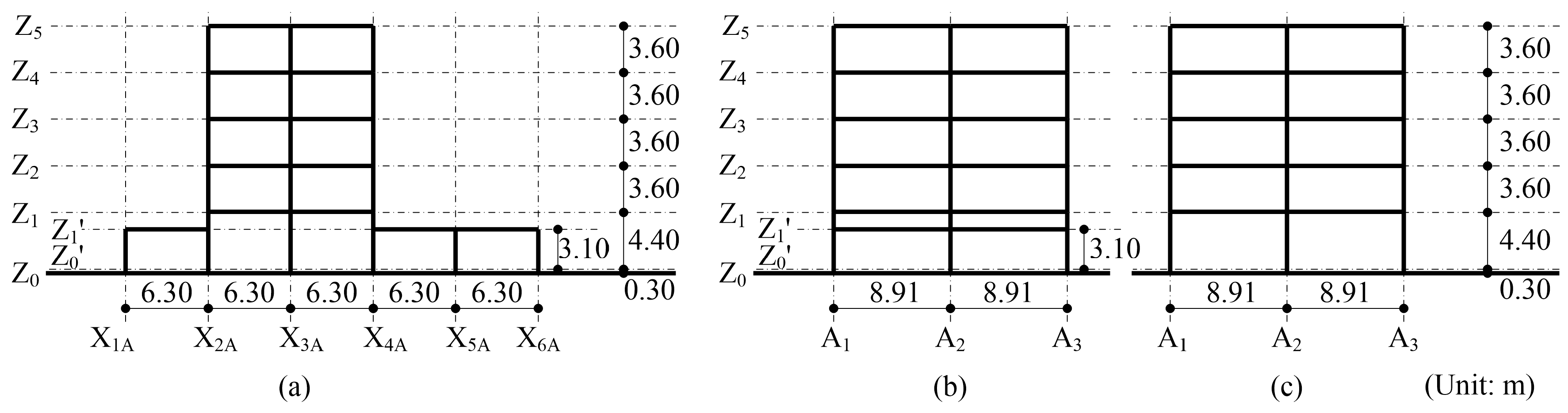
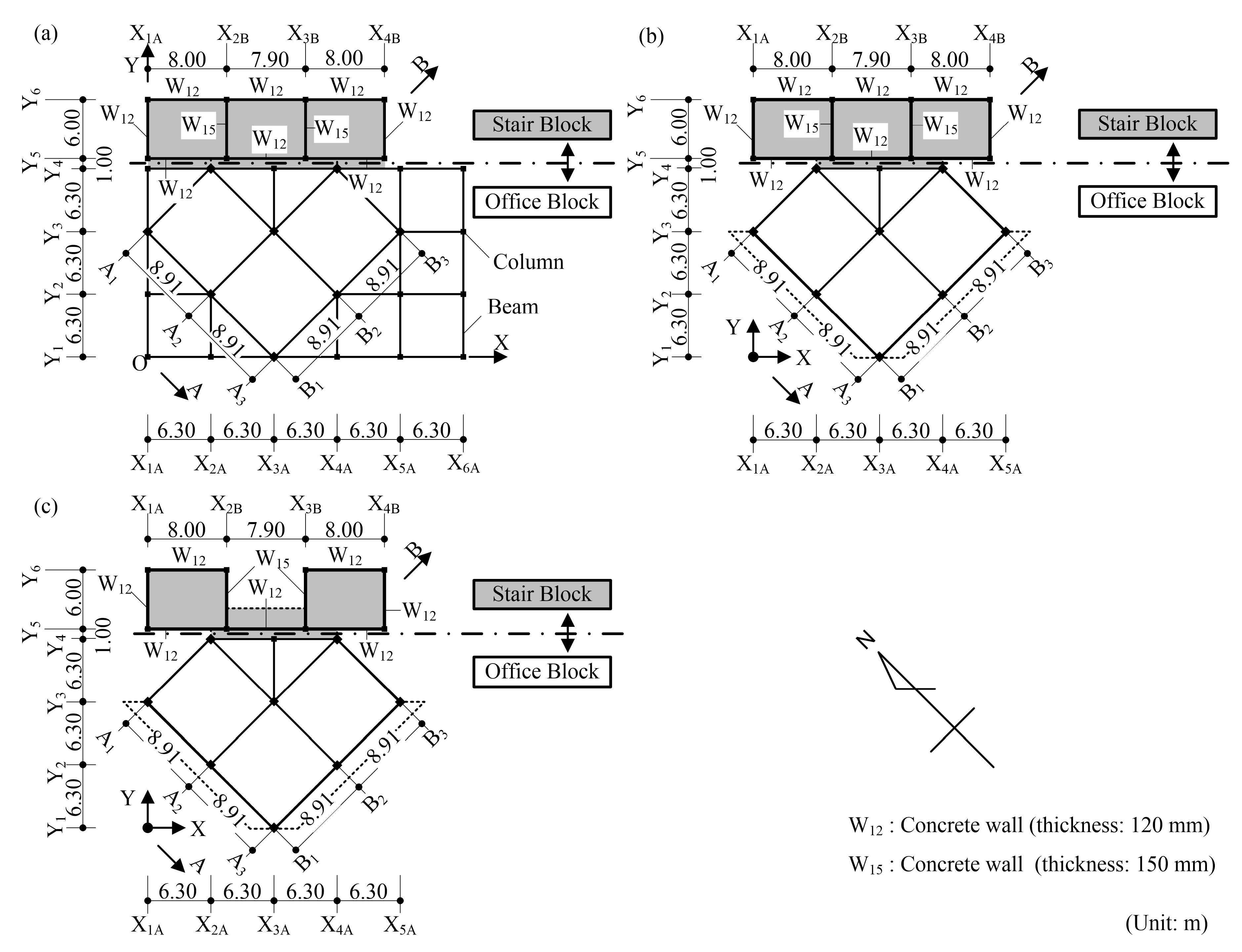
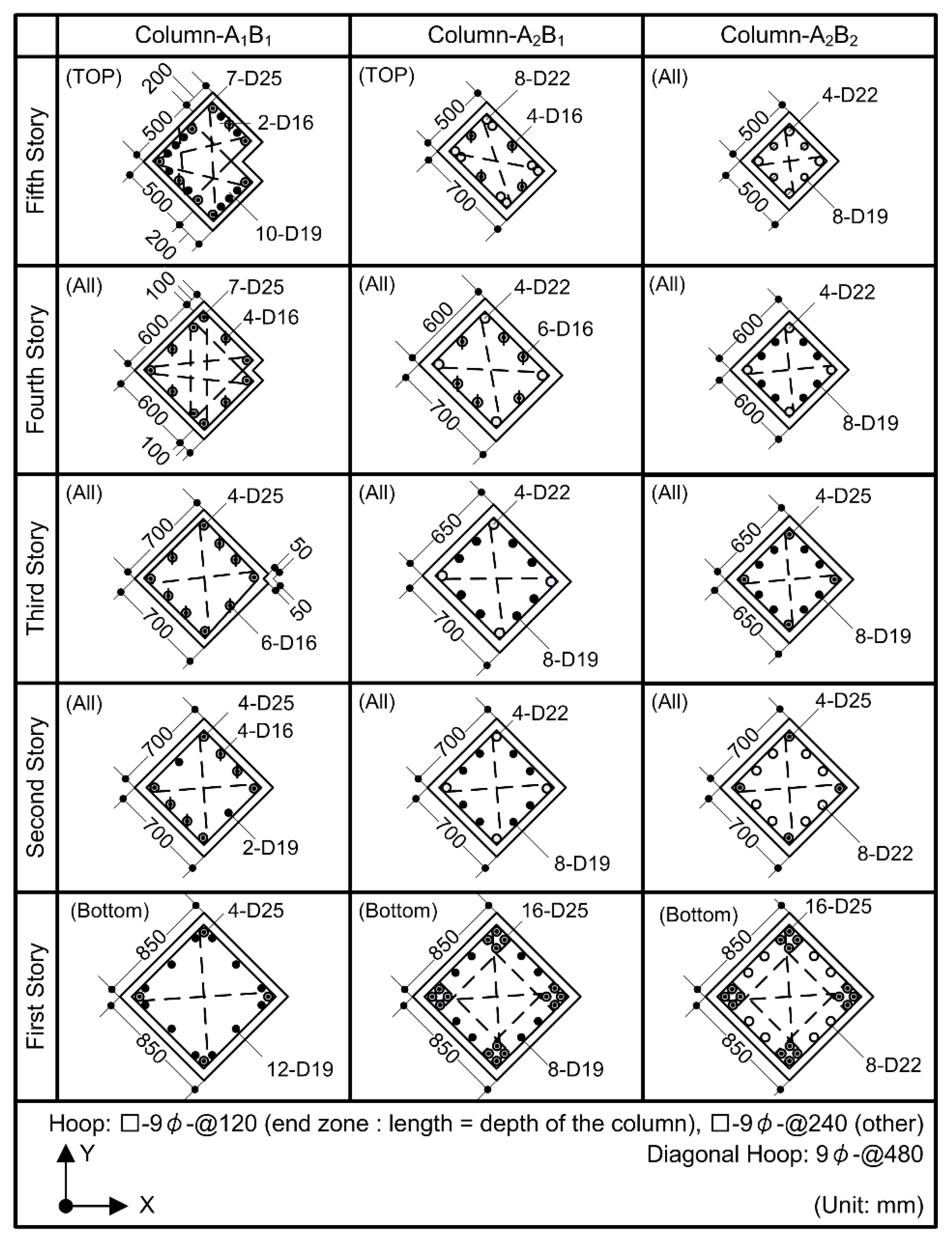
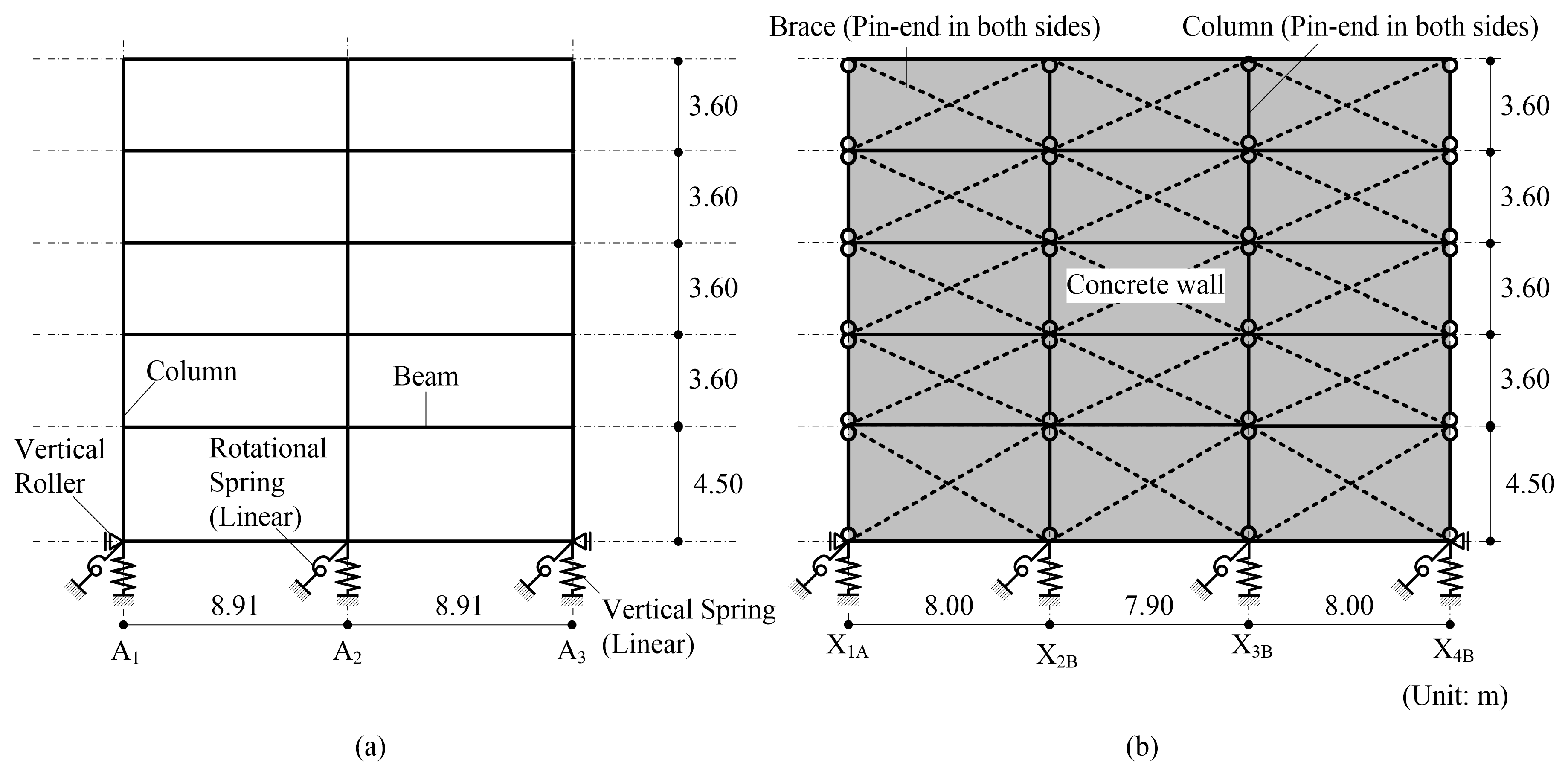
3.2. Analysis Model
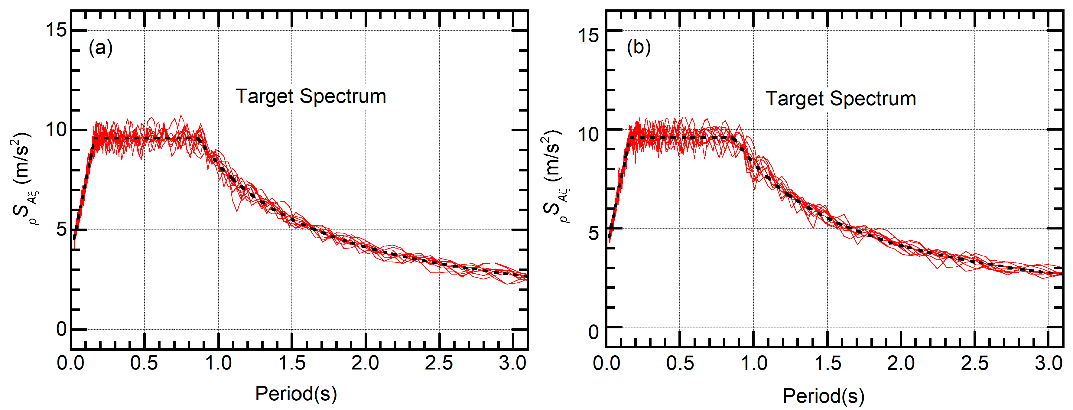
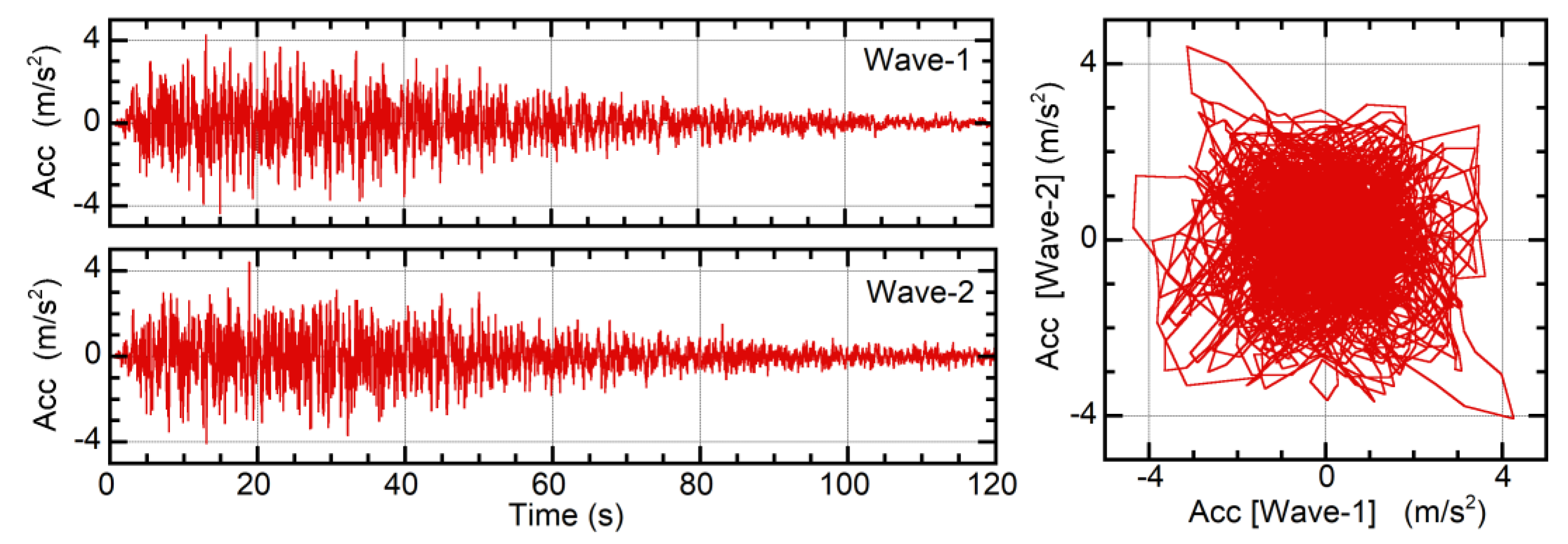
3.3. Ground Motion Data
4. Validation of the Seismic Capacity Evaluation Procedure
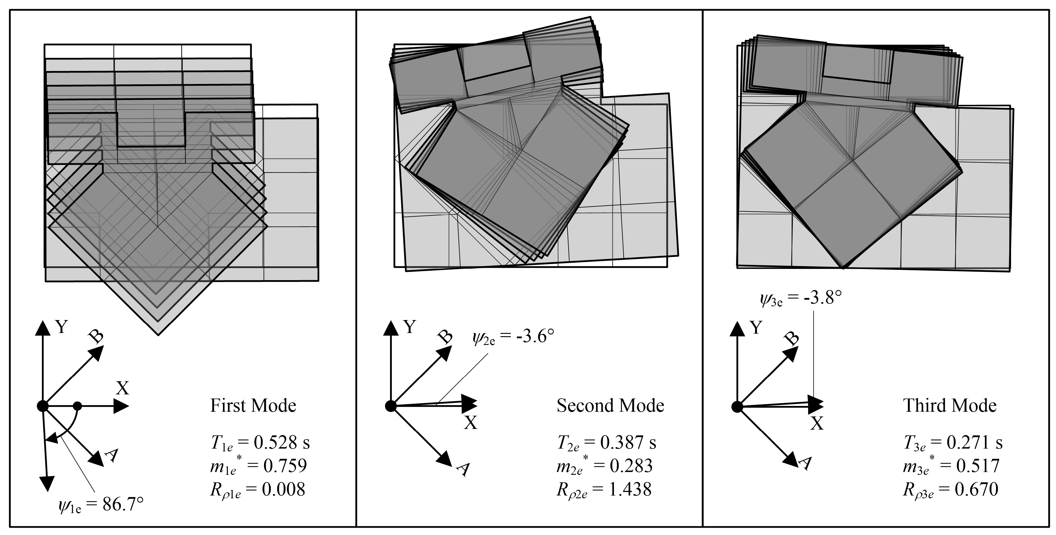
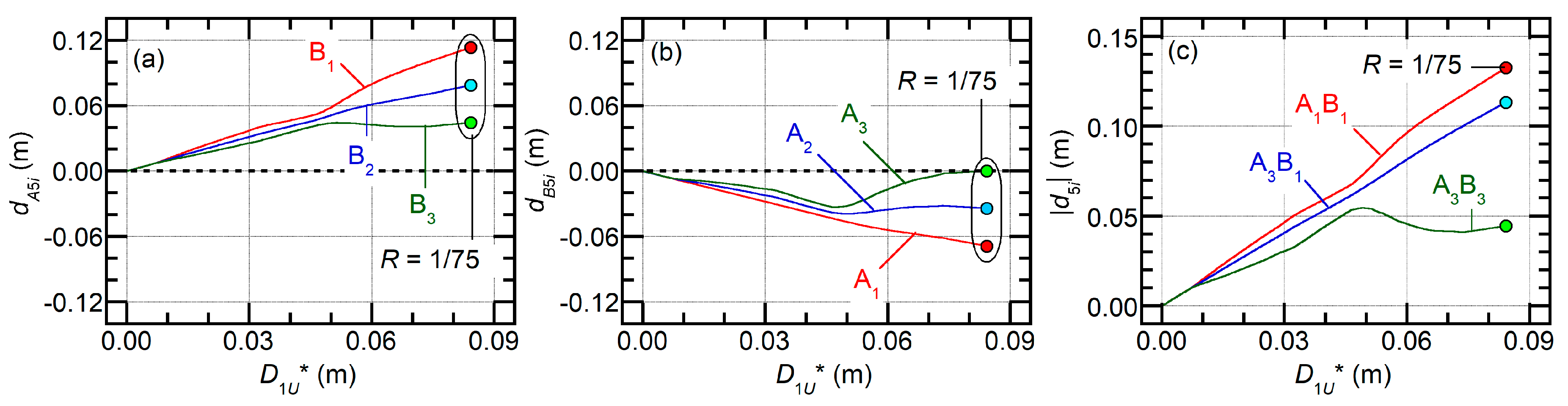
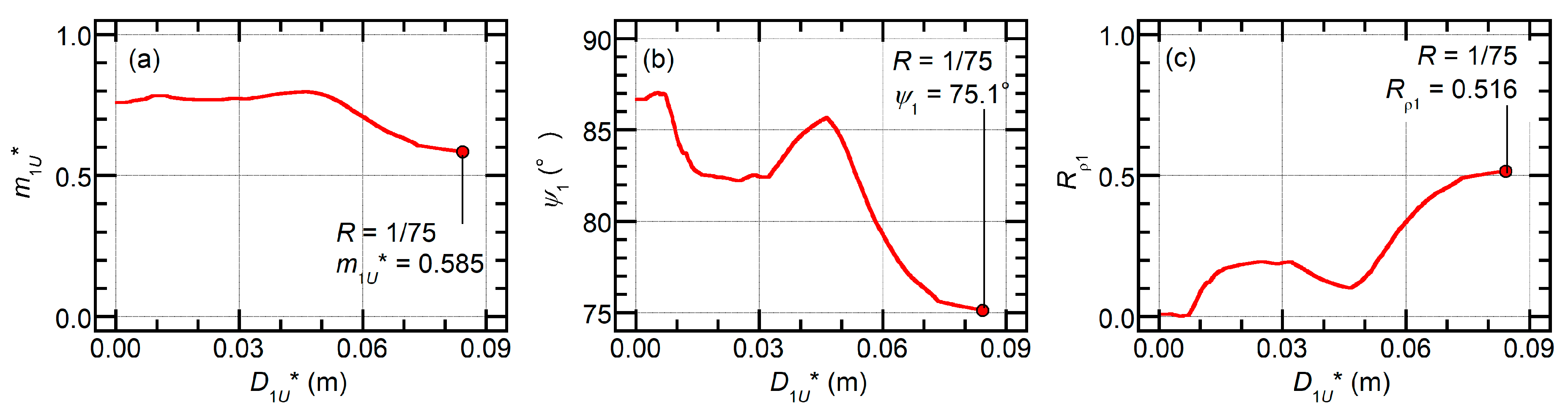
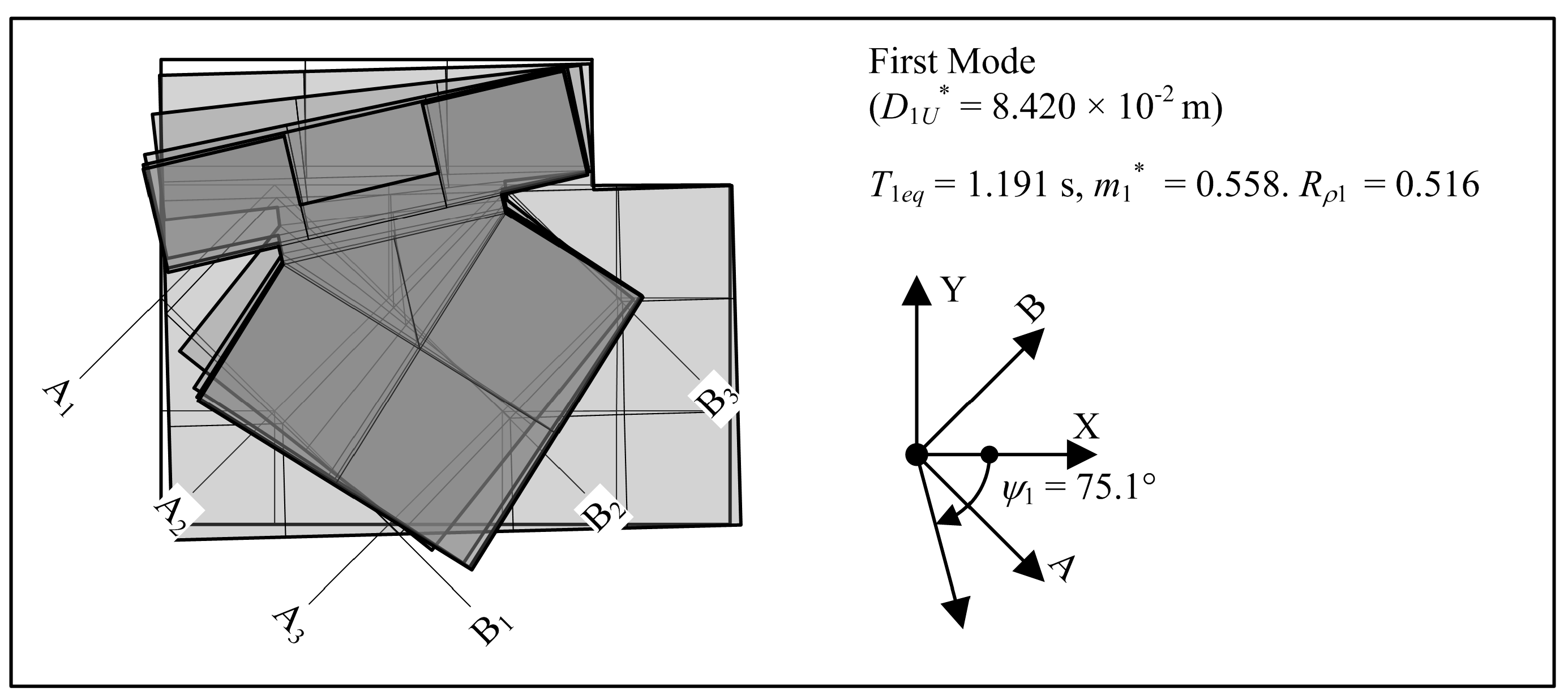
4.1. Pushover Analysis Results
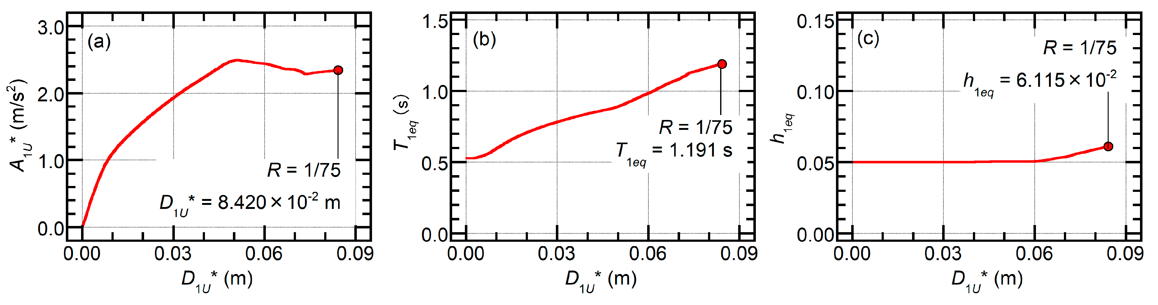
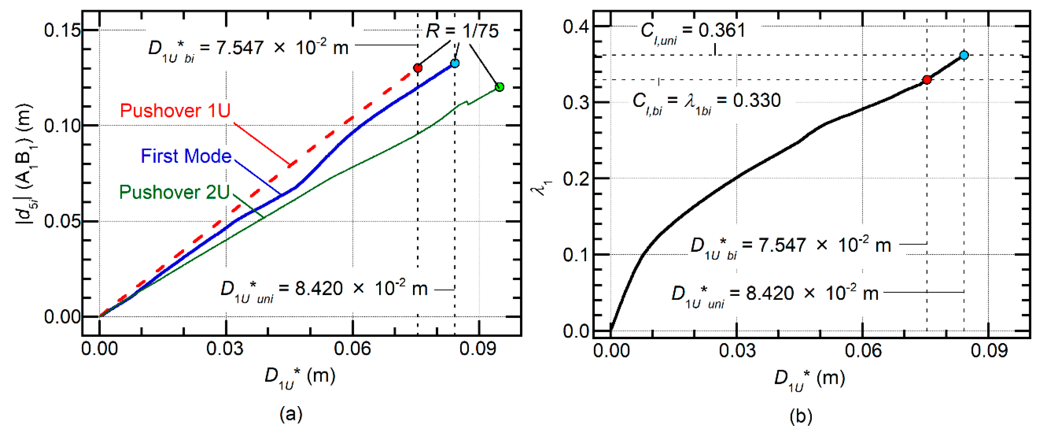
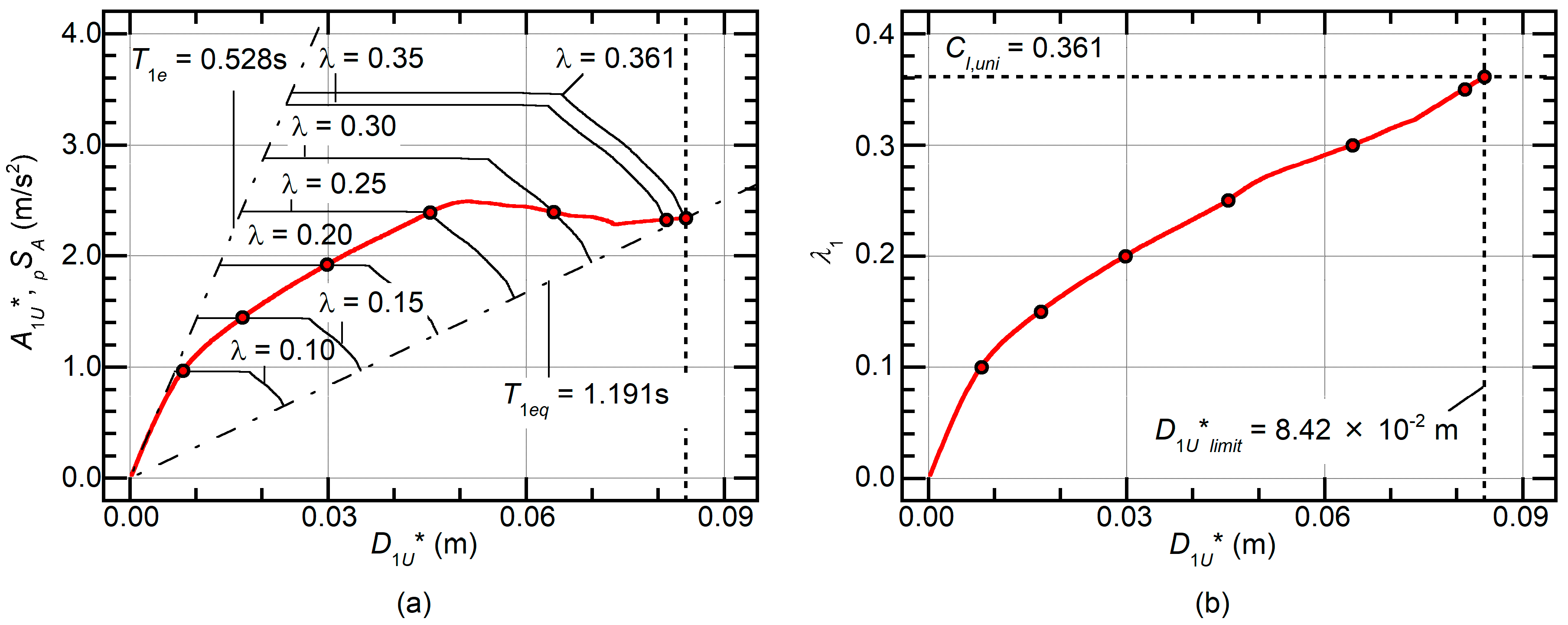
4.2. Evaluation of the Capacity Index
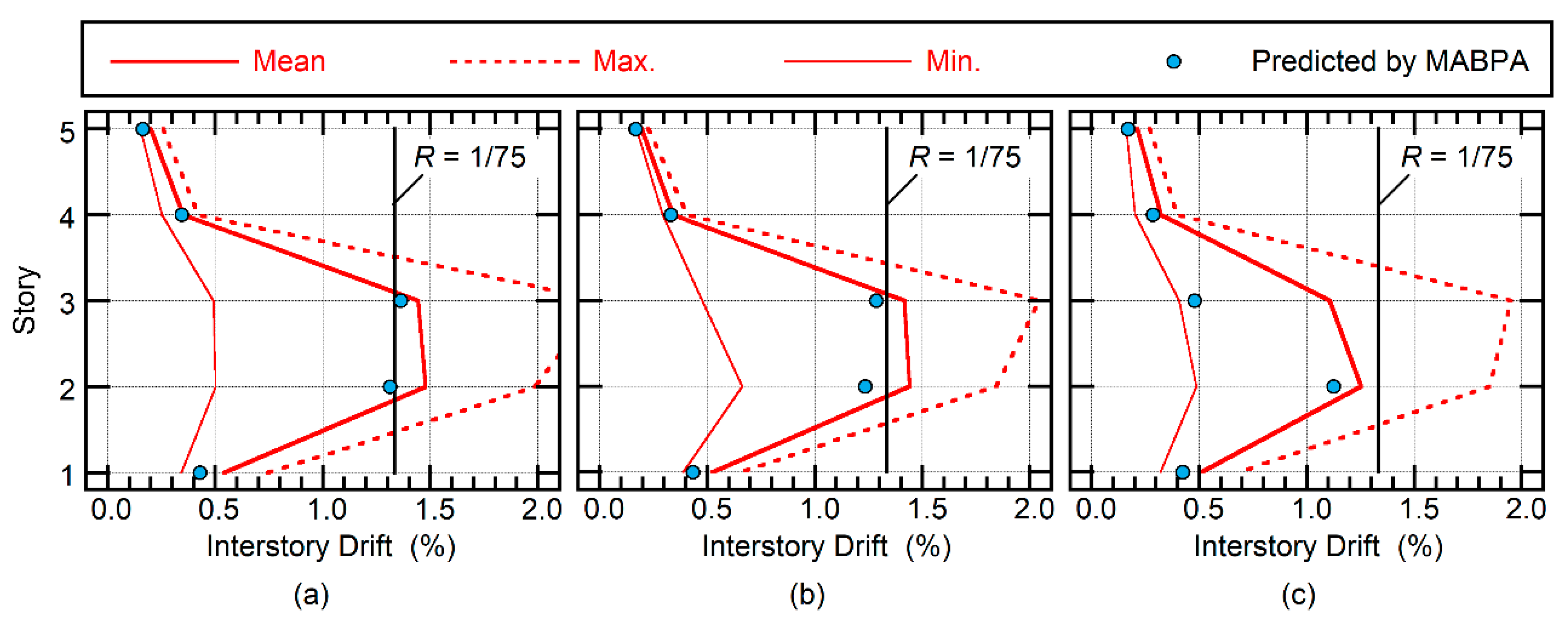
4.3. Validation of the Evaluation Procedure by Nonlinear Time-history Analysis
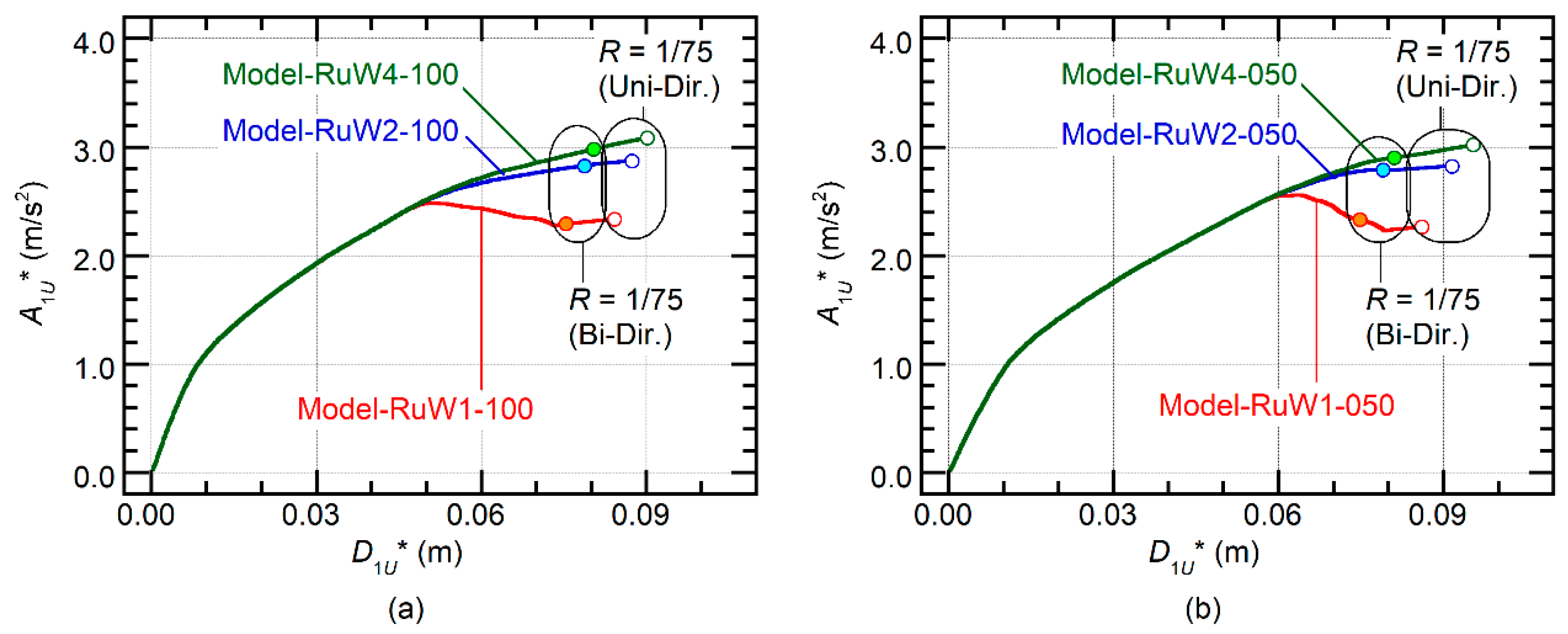
4.3.1. Analysis Cases
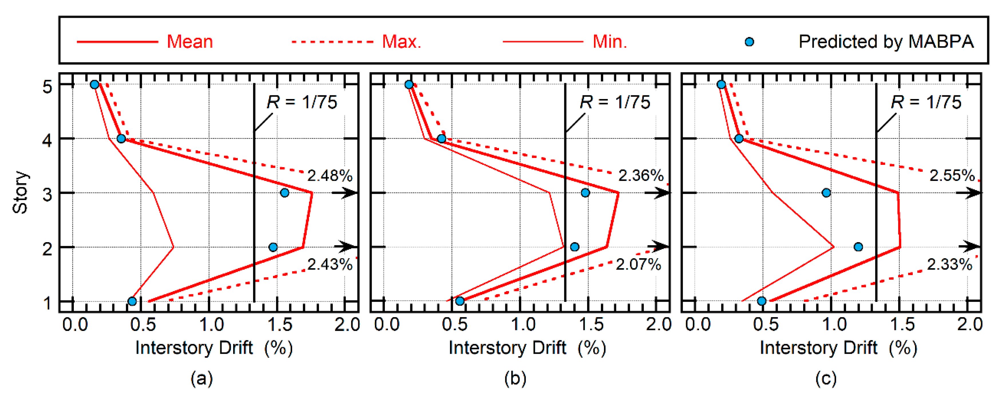
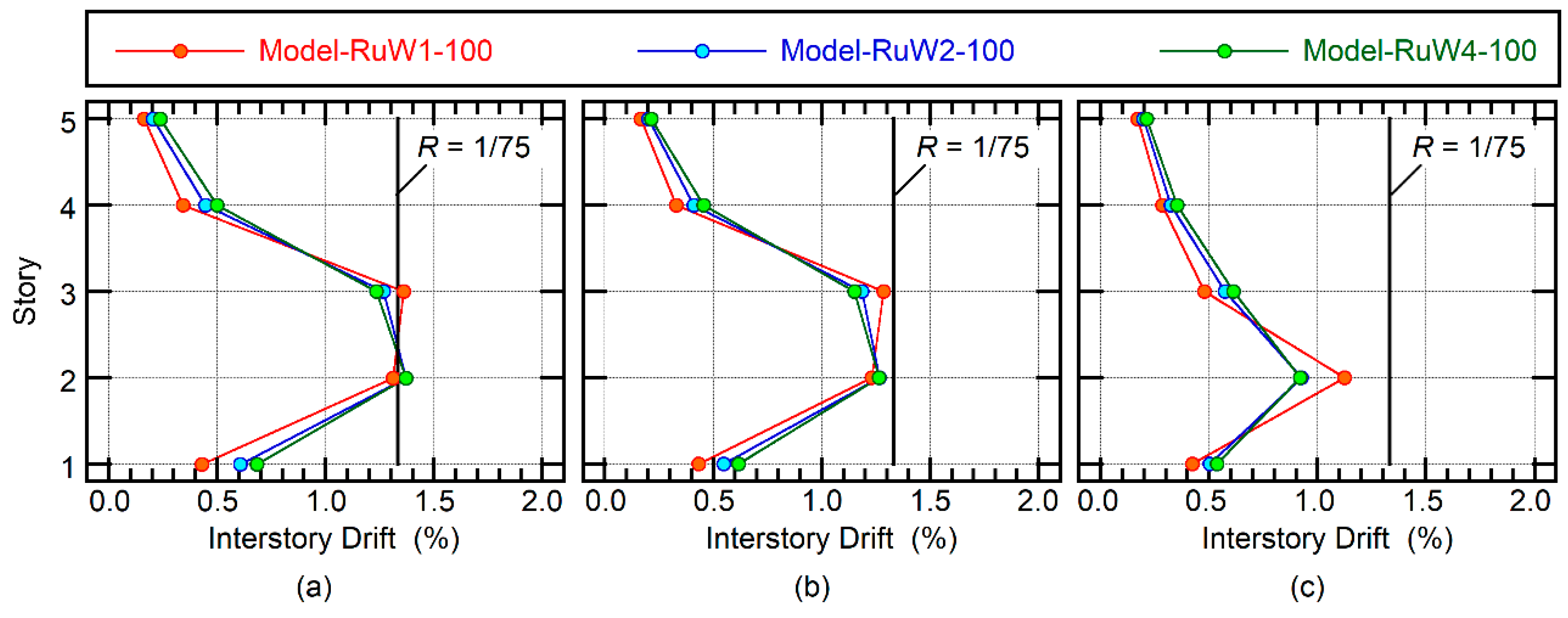
4.3.2. Analysis Results
5. Comparisons of the Evaluated Seismic Capacity of the Main Uto City Hall Building and the Response Spectrum of Recorded Earthquakes
5.1. Analysis Cases
5.2. Analysis Results
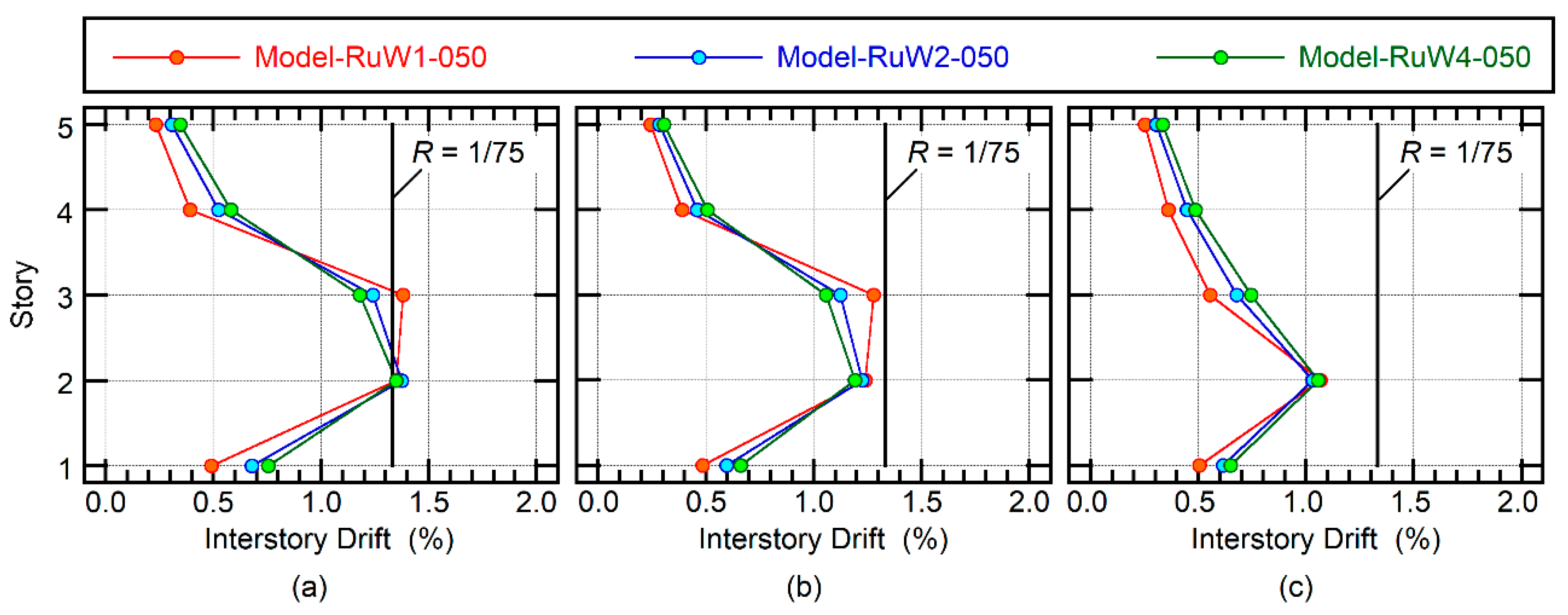
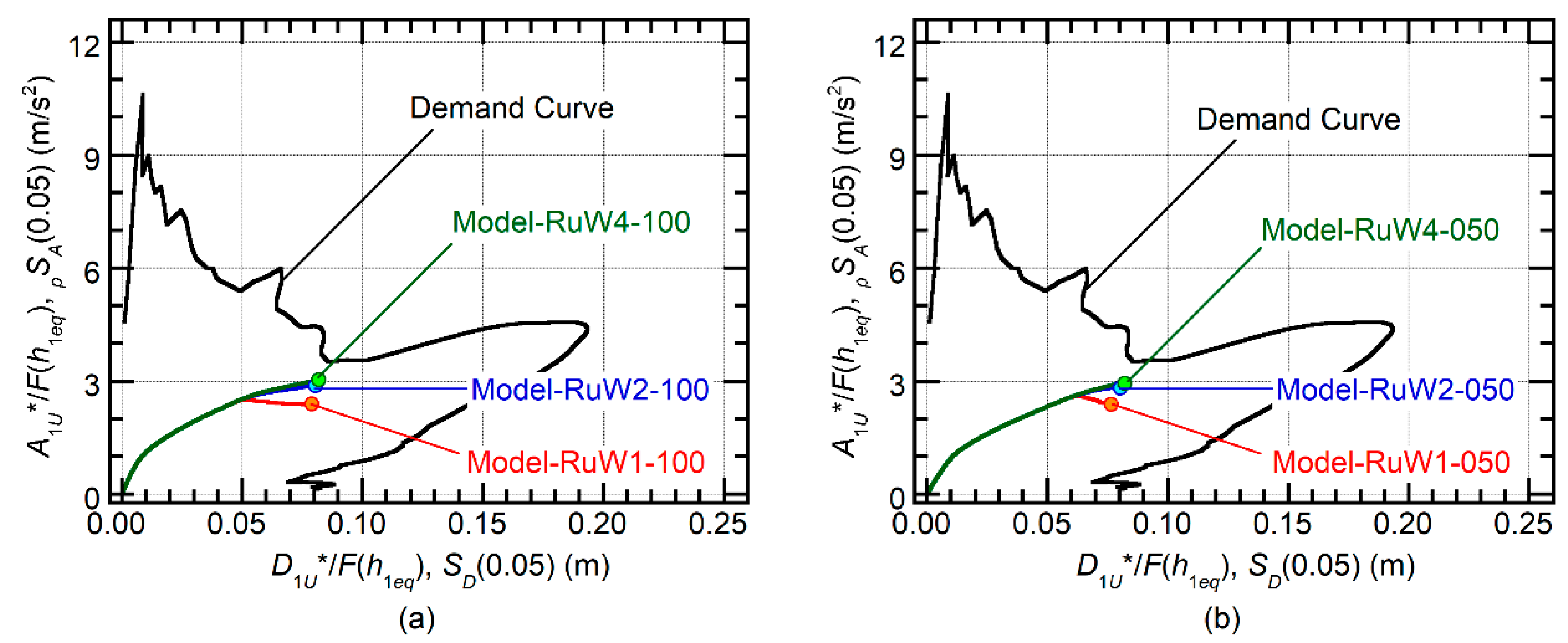
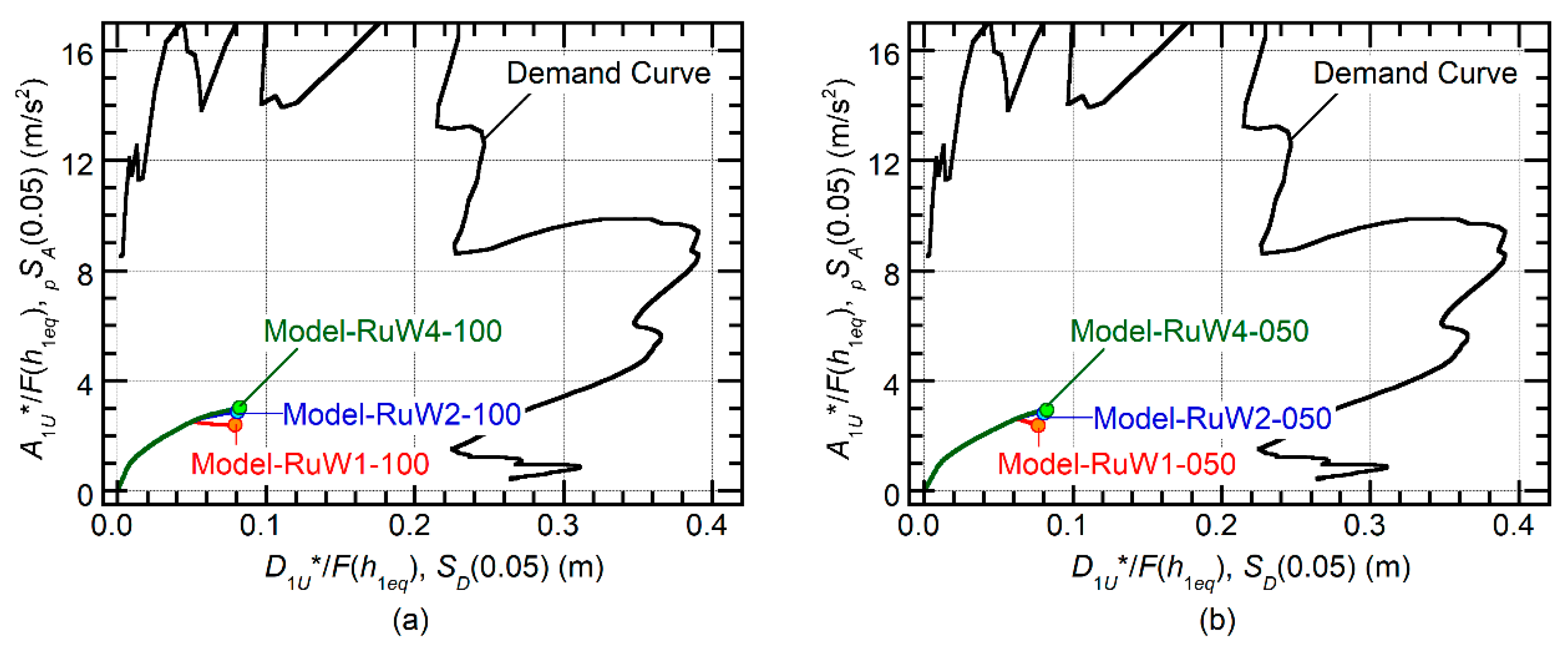
5.2.1. Capacity Curves and Seismic Capacity Indices
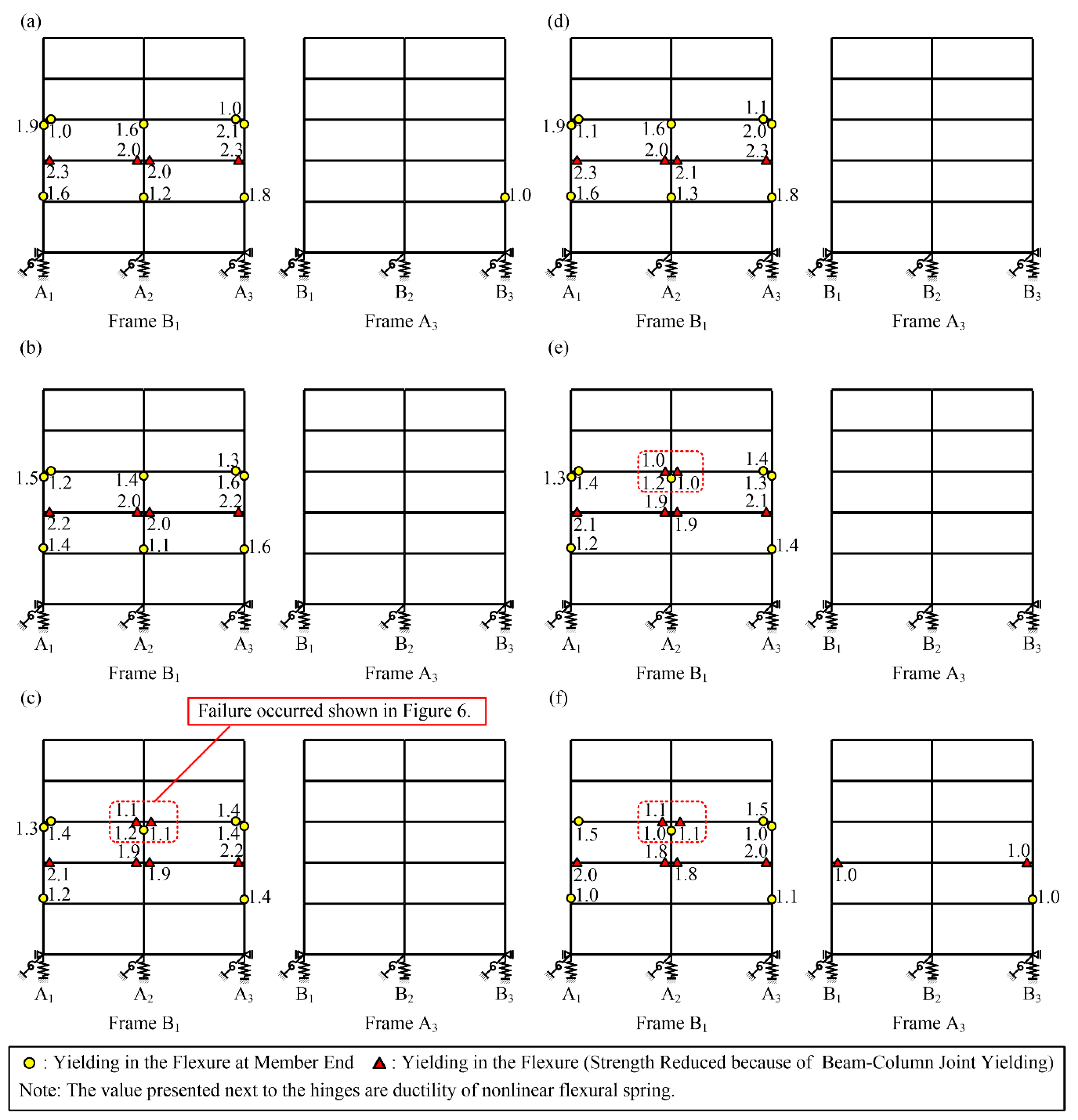
5.2.2. Calculated Peak Story Drift and the Structural Damages
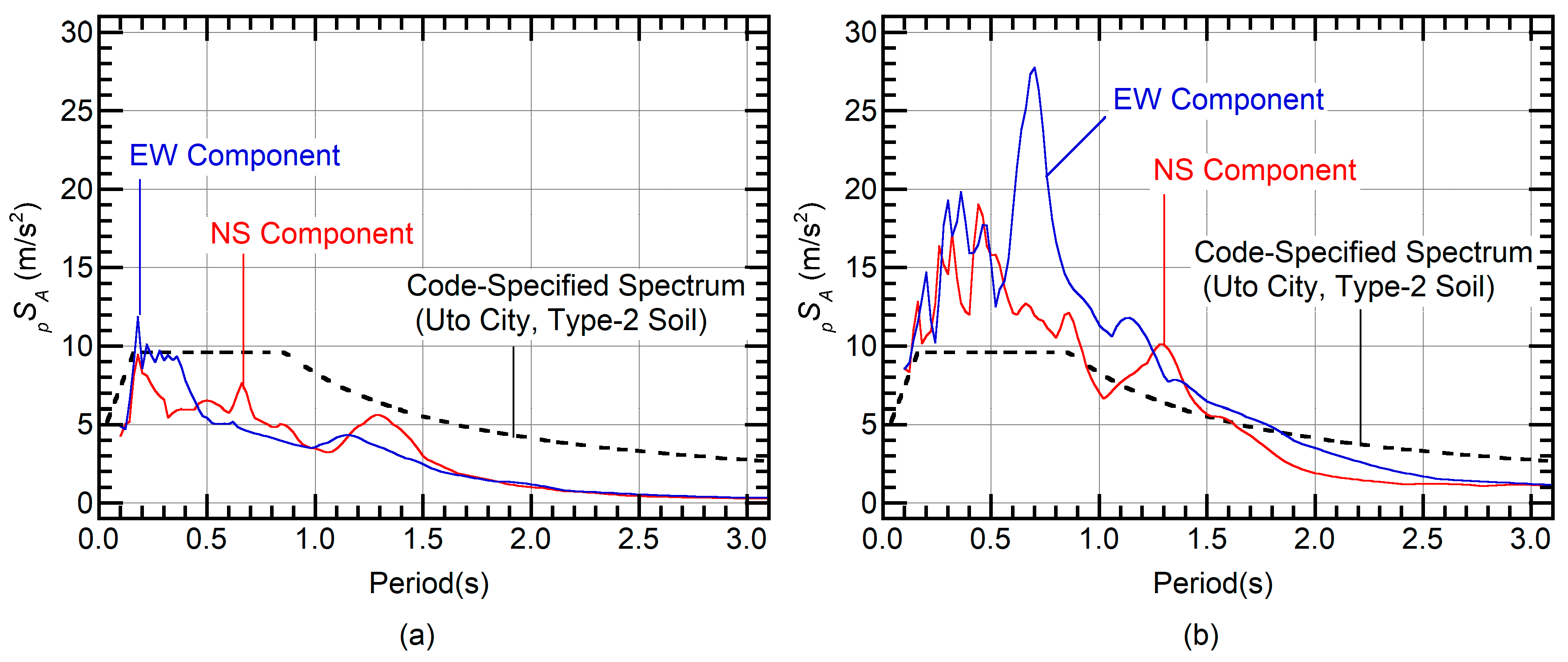
5.2.3. Comparisons with the Evaluated Seismic Capacity and the Response Spectrum of Recorded Earthquakes
5.3. Discussions
6. Conclusions
- A pushover-based procedure to evaluate the seismic capacity index considering bidirectional excitation is presented and its accuracy is verified by the nonlinear time-history analysis. The results show that the accuracy of the evaluated seismic capacity index for this building was satisfactory. Moreover, index CI, bi was better than index CI, uni because in this building, the effect of bidirectional excitation was significant.
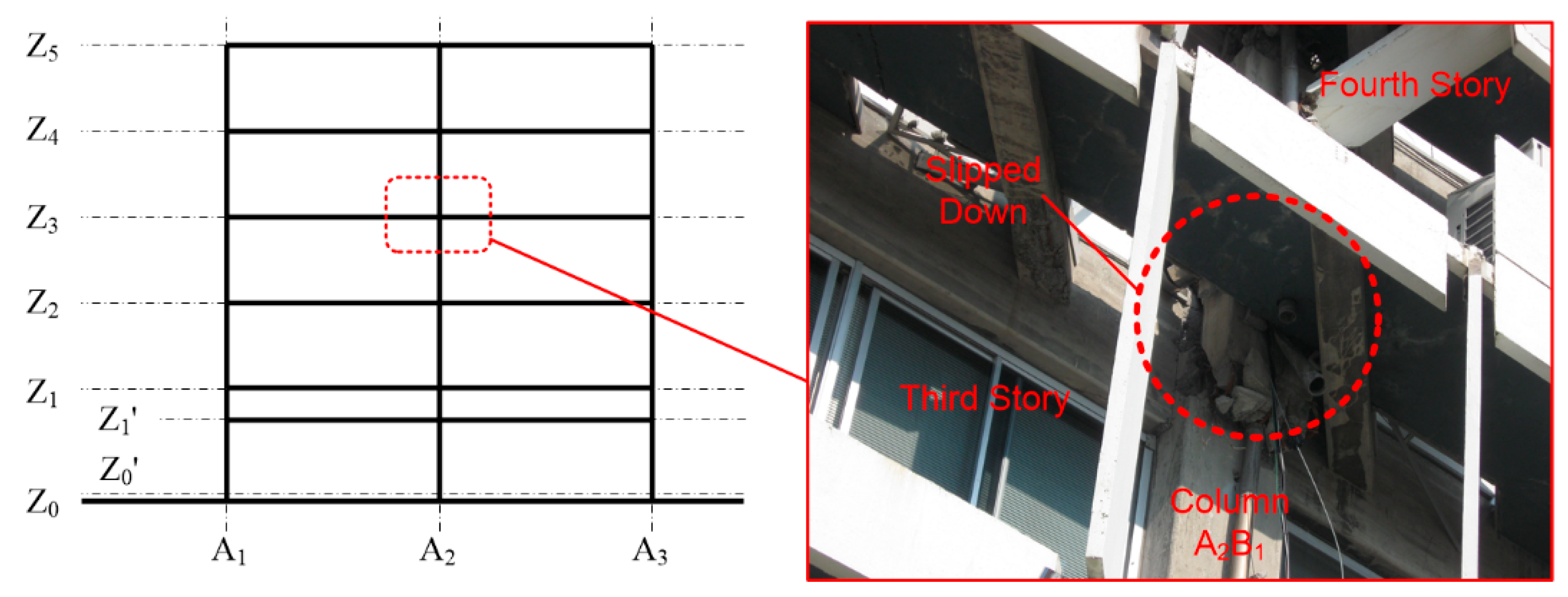
- The calculated damages of structural models presented in this paper may explain the part of the observed damage of the main Uto City Hall building during the 2016 Kumamoto Earthquake. The reason why the damage in frame B1 was more severe than that in frame A3 can be explained that, due to the effect of torsion, the response of frame B1 is more critical. Moreover, the severe failure of the beam-column joint at frame B1 observed above column A2B1 in the third story is consistent with the analysis results of the three analysis models presented in this paper.
- The seismic capacity index of the main Uto City Hall building evaluated by the proposed procedure is approximately 0.36 to 0.38. Therefore, this building could withstand only approximately one-third of the design ground motion specified in the current seismic code of Japan.
- During the first earthquake, which occurred on the 14 April, the main Uto City Hall building may suffer some structural damages, including the yielding of the beam-column joint. According to the comparison of the capacity curve of this building and the demand curve of the first earthquake, the capacity curve has no intersection point to the demand curve.
Author Contributions
Funding
Acknowledgments
Conflicts of Interest
Appendix A. Modification Factor for Predicting the Peak Response of The Equivalent SDOF Model Representing the Second Mode

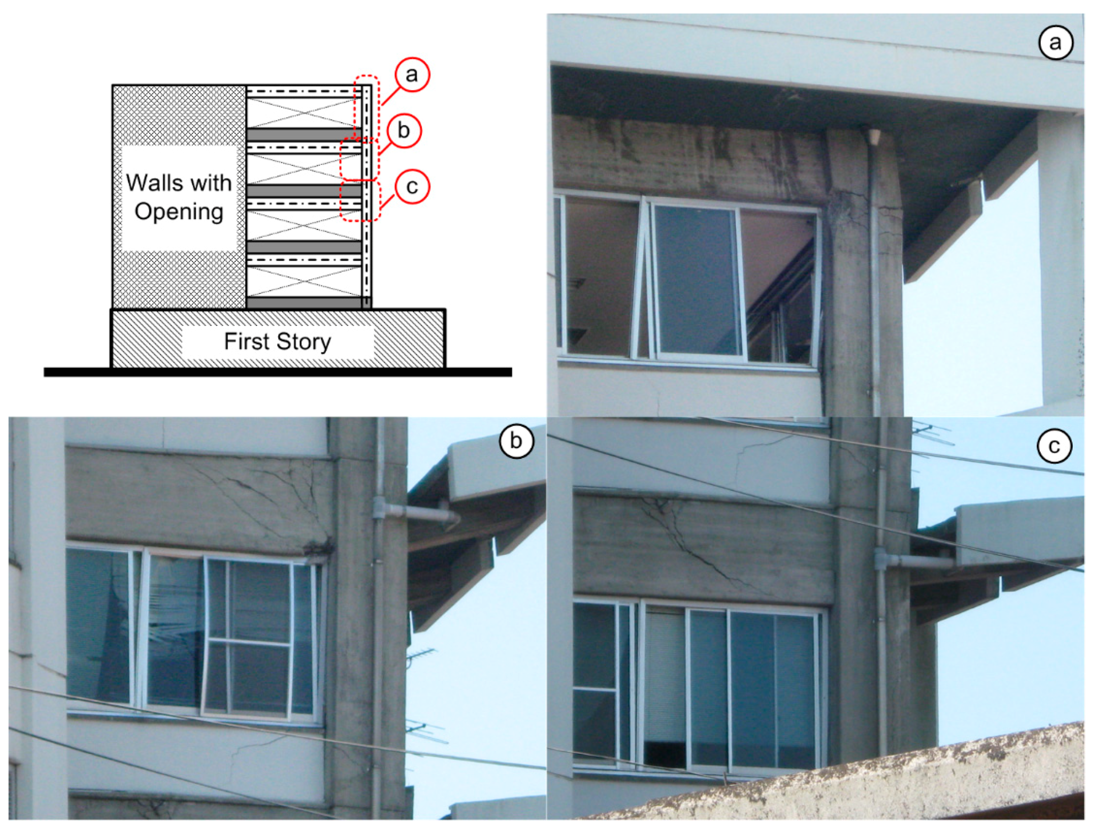
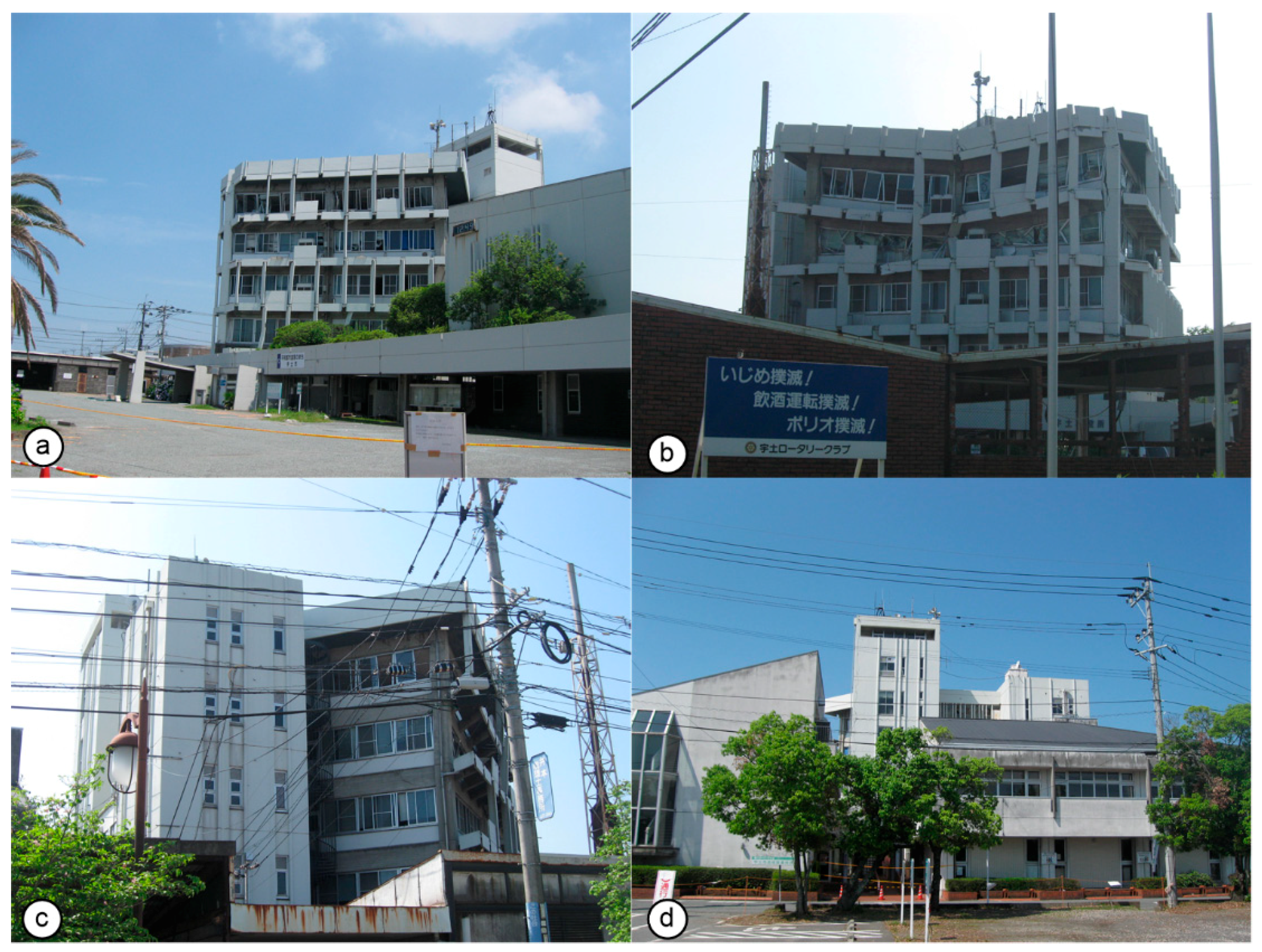
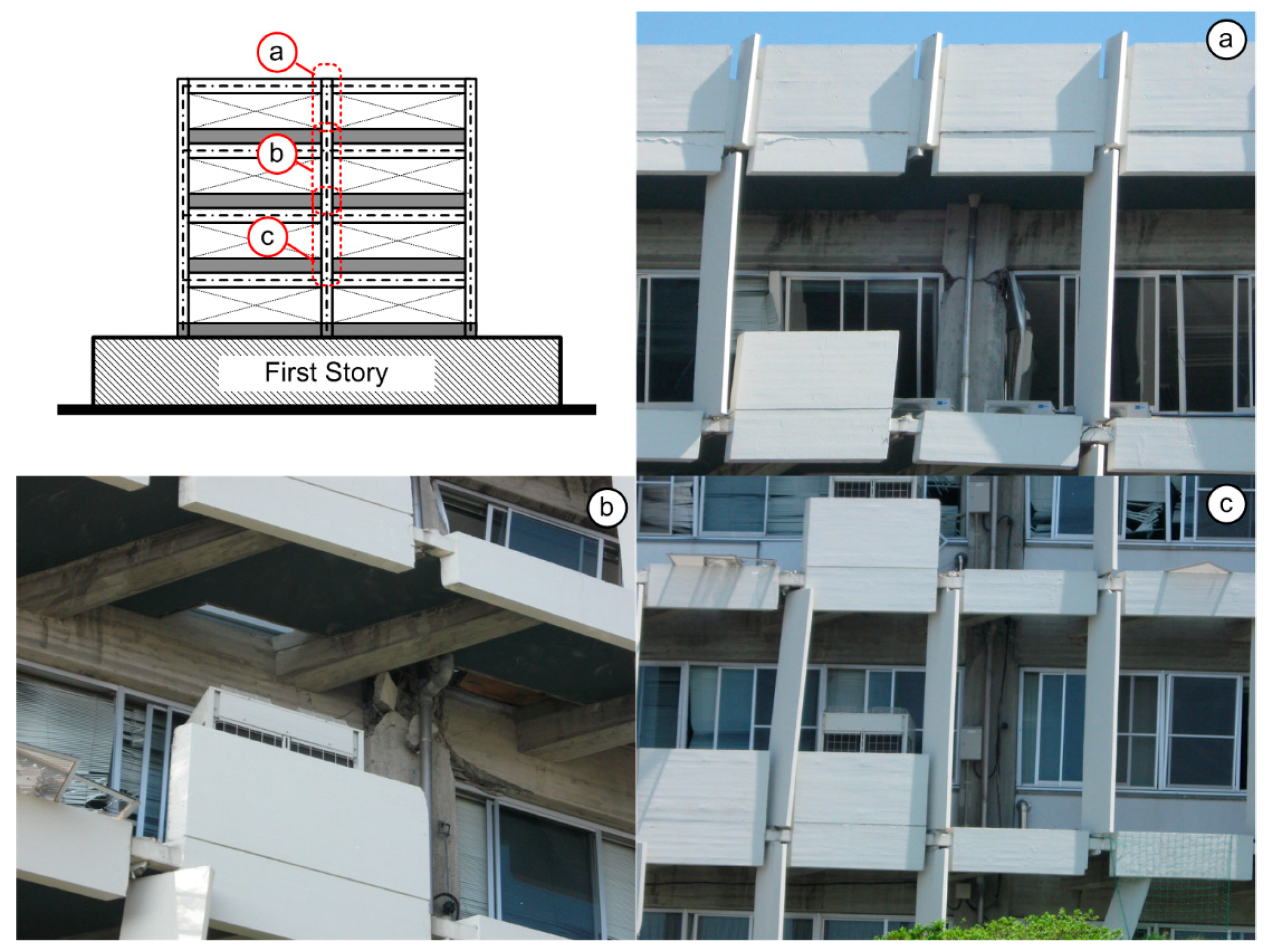
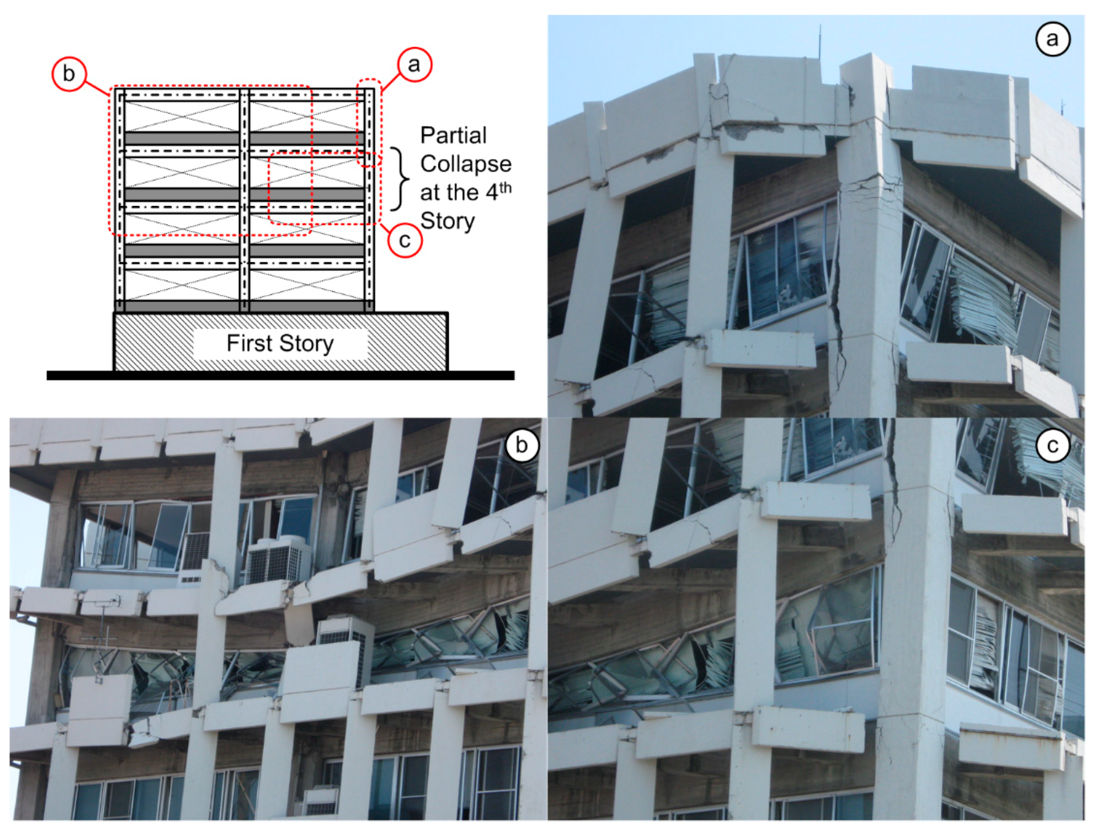
Appendix B. Building Damage


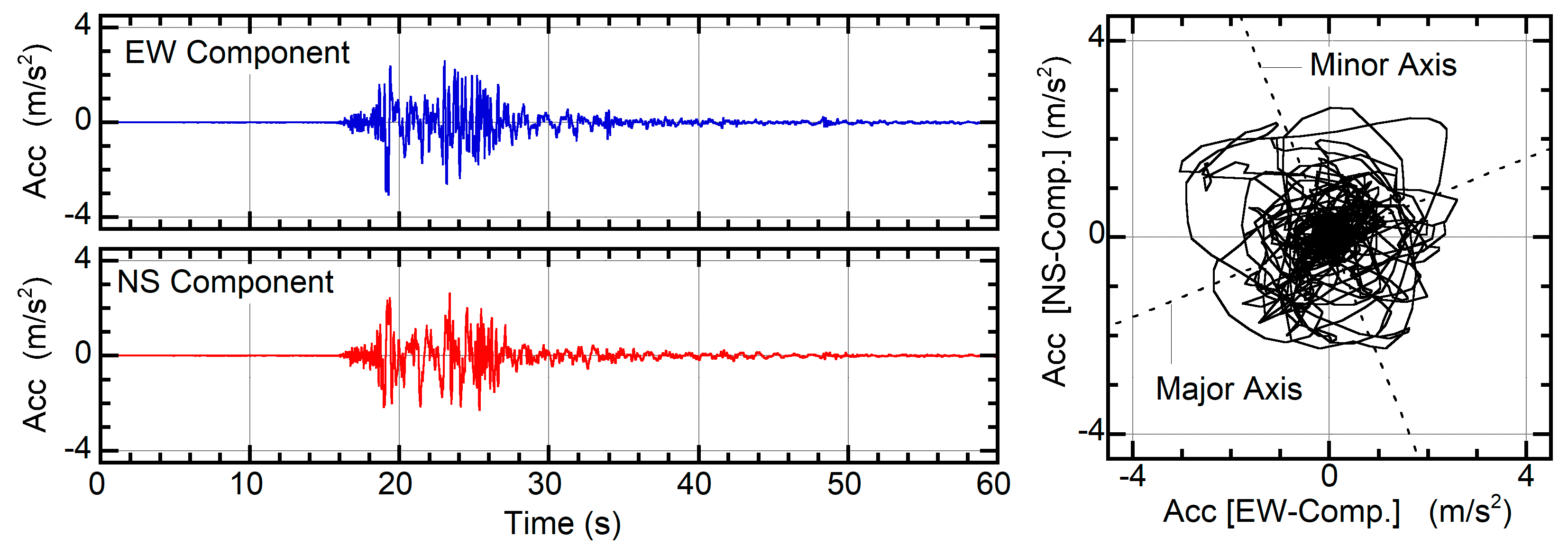
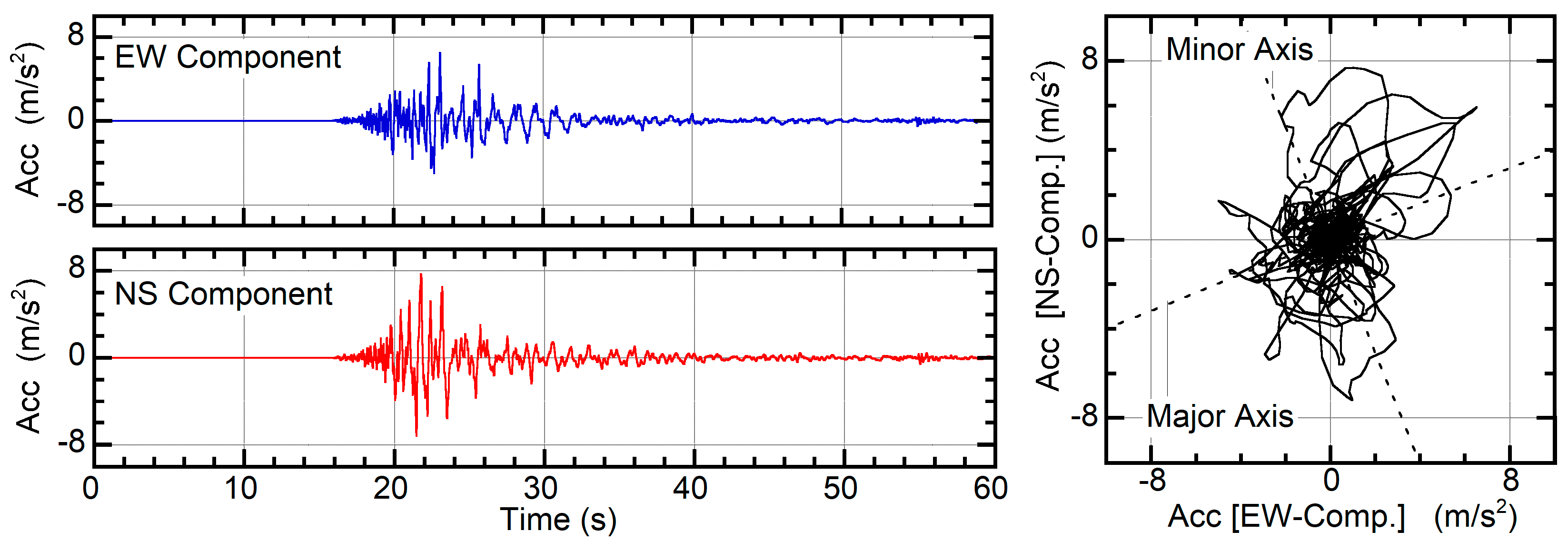
Appendix C. Record Observed in the 14th and 16th Earthquake at K-NET Uto Station


References
- Fujii, K.; Yoshida, S.; Nishimura, T.; Furuta, T. Observations of damage to Uto City Hall suffered in the 2016 Kumamoto Earthquake. In Proceedings of the 8th European Workshop on the Seismic Behaviour of Irregular and Complex Structures, Bucharest, Romania, 19–20 October 2017. [Google Scholar]
- Fujii, K. Preliminary evaluation of seismic capacity and torsional irregularity of Uto City Hall damaged in 2016 Kumamoto Earthquake. In Proceedings of the 8th European Workshop on the Seismic Behaviour of Irregular and Complex Structures, Bucharest, Romania, 19–20 October 2017. [Google Scholar]
- Saiidi, M.; Sozen, M.A. Simple nonlinear seismic analysis of R/C structures. J. Struct. Div. 1981, 107, 937–952. [Google Scholar]
- Fajfar, P.; Fischinger, M. N2-A method for non-linear seismic analysis of regular buildings. In Proceedings of the 9th World Conference on Earthquake Engineering, Tokyo-Kyoto, Japan, 2–9 August 1988. [Google Scholar]
- Fajfar, P. A nonlinear analysis method for performance-based seismic design. Earthq. Spectra 2000, 16, 573–592. [Google Scholar] [CrossRef]
- ATC-40. Seismic Evaluation and Retrofit of Concrete Buildings; Applied Technology Council: Redwood City, CA, USA, 1996; Volume 1. [Google Scholar]
- FEMA. NEHRP Guidelines for the Seismic Rehabilitation of Buildings; FEMA Publication 273; Federal Emergency Management Agency: Washington, DC, USA, 1997.
- CEN. Eurocode 8—Design of Structures for Earthquake Resistance. Part 1: General Rules, Seismic Actions and Rules for Buildings; European standard EN 1998-1; European Committee for Standardization: Brussels, Belgium, 2004. [Google Scholar]
- ASCE. Seismic Evaluation and Retrofit of Existing Buildings; ASCE standard, ASCE/SEI41-17; American Society of Civil Engineering: Reston, VA, USA, 2017. [Google Scholar]
- Peruŝ, I.; Fajfar, P. On the inelastic torsional response of single-storey structures under bi-axial excitation. Earthq. Eng. Struct. Dyn. 2005, 34, 931–941. [Google Scholar] [CrossRef]
- Fajfar, P.; Maruŝić, D.; Peruŝ, I. Torsional effects in the pushover-based seismic analysis of buildings. J. Earthq. Eng. 2005, 9, 831–854. [Google Scholar] [CrossRef]
- Kreslin, M.; Fajfar, P. Seismic evaluation of an existing complex RC building. Bull. Earthq. Eng. 2010, 8, 363–385. [Google Scholar] [CrossRef]
- Kreslin, M.; Fajfar, P. The extended N2 method considering higher mode effects in both plan and elevation. Bull. Earthq. Eng. 2012, 10, 695–715. [Google Scholar] [CrossRef]
- Dolšek, M.; Fajfar, P. Simplified probabilistic seismic performance assessment of plan-asymmetric buildings. Earthq. Eng. Struct. Dyn. 2007, 36, 2021–2041. [Google Scholar] [CrossRef]
- Chopra, A.K.; Goel, R.K. A modal pushover analysis procedure to estimate seismic demands for unsymmetric-plan buildings. Earthq. Eng. Struct. Dyn. 2004, 33, 903–927. [Google Scholar] [CrossRef] [Green Version]
- Reyes, J.C.; Chopra, A.K. Three-dimensional modal pushover analysis of buildings subjected to two components of ground motion, including its evaluation for tall buildings. Earthq. Eng. Struct. Dyn. 2011, 40, 789–806. [Google Scholar] [CrossRef]
- Reyes, J.C.; Chopra, A.K. Evaluation of three-dimensional modal pushover analysis for unsymmetric-plan buildings subjected to two components of ground motion. Earthq. Eng. Struct. Dyn. 2011, 40, 1475–1494. [Google Scholar] [CrossRef]
- Manoukas, G.; Athanatopoulou, A.; Avramidis, I. Multimode pushover analysis for asymmetric buildings under biaxial seismic excitation based on a new concept of the equivalent single degree of freedom system. Soil Dyn. Earthq. Eng. 2012, 38, 88–96. [Google Scholar] [CrossRef]
- Manoukas, G.; Avramidis, I. Evaluation of a multimode pushover procedure for asymmetric in plan buildings under biaxial seismic excitation. Bull. Earthq. Eng. 2014, 12, 2607–2632. [Google Scholar] [CrossRef]
- Belejo, A.; Bento, R. Improved modal pushover analysis in seismic assessment of asymmetric plan buildings under the influence of one and two horizontal components of ground motions. Soil Dyn. Earthq. Eng. 2016, 87, 1–15. [Google Scholar] [CrossRef]
- Soleimani, S.; Aziminejad, A.; Moghadam, A.S. Extending the concept of energy-based pushover analysis to assess seismic demands of asymmetric-plan buildings. Soil Dyn. Earthq. Eng. 2017, 93, 29–41. [Google Scholar] [CrossRef]
- Reyes, J.C.; Riaño, A.C.; Kalkan, E.; Arango, C.M. Extending modal pushover-based scaling procedure for nonlinear response history analysis of multi-story unsymmetric-plan buildings. Eng. Struct. 2015, 88, 125–137. [Google Scholar] [CrossRef]
- Bosco, M.; Ghersi, A.; Marino, E.M. Corrective eccentricities for assessment by nonlinear static method of 3D structures subjected to bidirectional ground motion. Earthq. Eng. Struct. Dyn. 2012, 41, 1751–1773. [Google Scholar] [CrossRef]
- Bosco, M.; Ferrara, G.A.F.; Ghersi, A.; Marino, E.M.; Rossi, P.P. Predicting displacement demand of multi-storey asymmetric buildings by nonlinear static analysis and corrective eccentricities. Eng. Struct. 2015, 99, 373–387. [Google Scholar] [CrossRef]
- Fujii, K. Nonlinear static procedure for multi-story asymmetric frame buildings considering bi-directional excitation. J. Earthq. Eng. 2011, 15, 245–273. [Google Scholar] [CrossRef]
- Fujii, K. Prediction of the largest peak nonlinear seismic response of asymmetric buildings under bi-directional excitation using pushover analyses. Bull. Earthq. Eng. 2014, 12, 909–938. [Google Scholar] [CrossRef]
- Fujii, K. Application of the pushover-based procedure to predict the largest peak response of asymmetric buildings with buckling-restrained braces. In Proceedings of the 5th International Conference on Computational Methods in Structural Dynamics and Earthquake Engineering (COMPDYN 2015), Crete Island, Greece, 25–27 May 2015. [Google Scholar]
- Fujii, K. Assessment of pushover-based method to a building with bidirectional setback. Earthq. Struct. 2016, 11, 421–443. [Google Scholar] [CrossRef]
- Fujii, K. Prediction of the peak seismic response of asymmetric buildings under bidirectional horizontal ground motion using equivalent SDOF model. Jpn. Archit. Rev. 2018, 1, 29–43. [Google Scholar] [CrossRef] [Green Version]
- López, A.; Torres, R. The critical angle of seismic incidence and the maximum structural response. Earthq. Eng. Struct. Dyn. 1997, 26, 881–894. [Google Scholar] [CrossRef]
- López, A.; Hernández, J.J.; Bonilla, R.; Fernández, A. Response spectra for multicomponent structural analysis. Earthq. Spectra 2006, 22, 85–113. [Google Scholar] [CrossRef]
- NZSEE/MBIE. The Seismic Assessment of Existing Buildings. Technical Guidelines for Engineering Assessments. Part A: Assessment Objectives and Principles. New Zealand Society for Earthquake Engineering: Wellington, 2017. Available online: www.EQ-Assess.org.nz (accessed on 26 February 2019).
- NZSEE/MBIE. The Seismic Assessment of Existing Buildings. Technical Guidelines for Engineering Assessments. Part B: Initial Seismic Assessment. New Zealand Society for Earthquake Engineering: Wellington, 2017. Available online: www.EQ-Assess.org.nz (accessed on 26 February 2019).
- NZSEE/MBIE. The Seismic Assessment of Existing Buildings. Technical Guidelines for Engineering Assessments. Part C: Detailed Seismic Assessment. New Zealand Society for Earthquake Engineering: Wellington, 2017. Available online: www.EQ-Assess.org.nz (accessed on 26 February 2019).
- Vecchio, C.D.; Gentile, R.; Ludovico, M.D.; Uva, G.; Pampanin, S. Implementation and Validation of the Simple Lateral Mechanism Analysis (SLaMA) for the Seismic Performance Assessment of a Damaged Case Study Building. J. Earthq. Eng. 2018, 1–32. Available online: www.tandfonline.com (accessed on 26 February 2019). [CrossRef]
- Otani, S. New seismic design provision in Japan. In Proceedings of the Second U.S.-Japan Workshop on Performance-Based Earthquake Engineering Methodology for Reinforced Concrete Structures, PEER Report. Sapporo, Hokkaido, Japan, 3–14 October 2000. [Google Scholar]
- Shiga, T. Earthquake damage and the amount of walls in reinforced concrete buildings. In Proceedings of the 6th World Conference on Earthquake Engineering, New Delhi, India, 9–14 January 1977. [Google Scholar]
- AIJ. AIJ Standard for Lateral Load-Carrying Capacity Calculation of Reinforced Concrete Structures (Draft); Architectural Institute of Japan: Tokyo, Japan, 2016. (In Japanese) [Google Scholar]
- Sugano, S.; Koreishi, I. An empirical evaluation of inelastic behaviour of structural elements in reinforced concrete frames subjected to lateral forces. In Proceedings of the 5th World Conference on Earthquake Engineering, Rome, Italy, 25–29 June 1974; Volume 1, pp. 841–844. [Google Scholar]
- Muto, K.; Hisada, T.; Tsugawa, T.; Bessho, S. Earthquake resistant design of a 20 story reinforced concrete buildings. In Proceedings of the 5th World Conference on Earthquake Engineering, Rome, Italy, 25–29 June 1974; Volume 2, pp. 1960–1969. [Google Scholar]
- Otani, S. Hysteresis models of reinforced concrete for earthquake response analysis. J. Fac. Eng. 1981, 36, 125–156. [Google Scholar]
- BRI; BCJ. Guideline for the Generation of Earthquake Motions for Seismic Design of Buildings (Draft); The Building Center of Japan, 1993. (In Japanese). Available online: www.bcj.or.jp/download/wave/ (accessed on 27 July 2010).
- Otani, S. Japanese seismic design of high-rise reinforced concrete buildings—An example of performance-based design code and state of practices. In Proceedings of the 13th World Conference on Earthquake Engineering, Vancouver, Canada, 1–6 August 2004. Paper No. 5010. [Google Scholar]
- Boore, D.M.; Watson-Lamprey, J.; Abrahamson, N.A. Orientation-Independent Measures of Ground Motion. Bull. Seismol. Soc. Am. 2007, 96, 1502–1511. [Google Scholar] [CrossRef]
- Strong-Motion Seismograph Network (K-NET, KIK-NET) Home Page. Available online: www.kyoshin.bosai.go.jp/kyoshin/ (accessed on 4 May 2016).
- Penzien, J.; Watabe, M. Characteristics of 3-Dimensional Earthquake Ground Motions. Earthq. Eng. Struct. Dyn. 1975, 3, 365–373. [Google Scholar] [CrossRef]


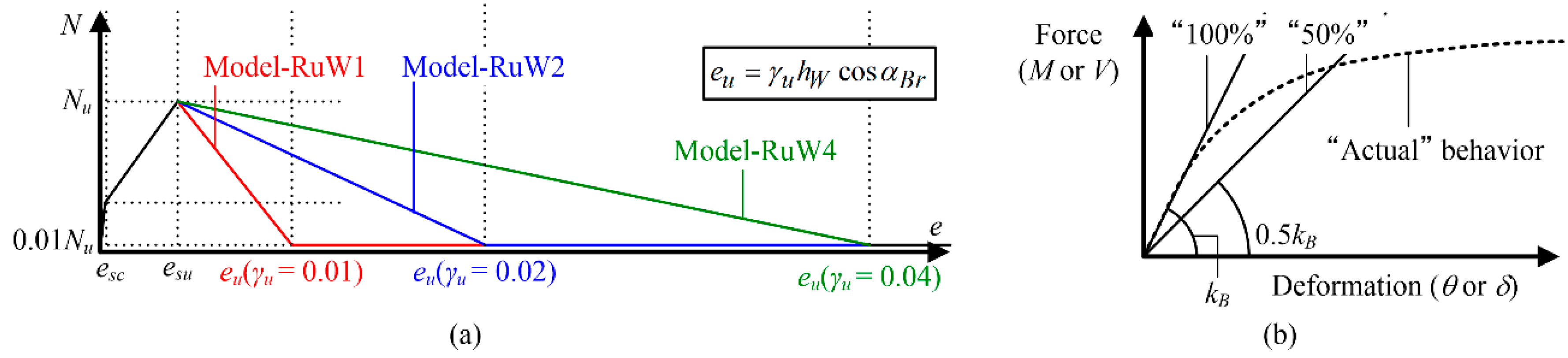
| Model ID | Shear Strain γu | Stiffness Ratio of Spring at Each Basement |
|---|---|---|
| Model-RuW1-100 | 0.01 | 100% |
| Model-RuW2-100 | 0.02 | |
| Model-RuW4-100 | 0.04 | |
| Model-RuW1-050 | 0.01 | 50% |
| Model-RuW2-050 | 0.02 | |
| Model-RuW4-050 | 0.04 |
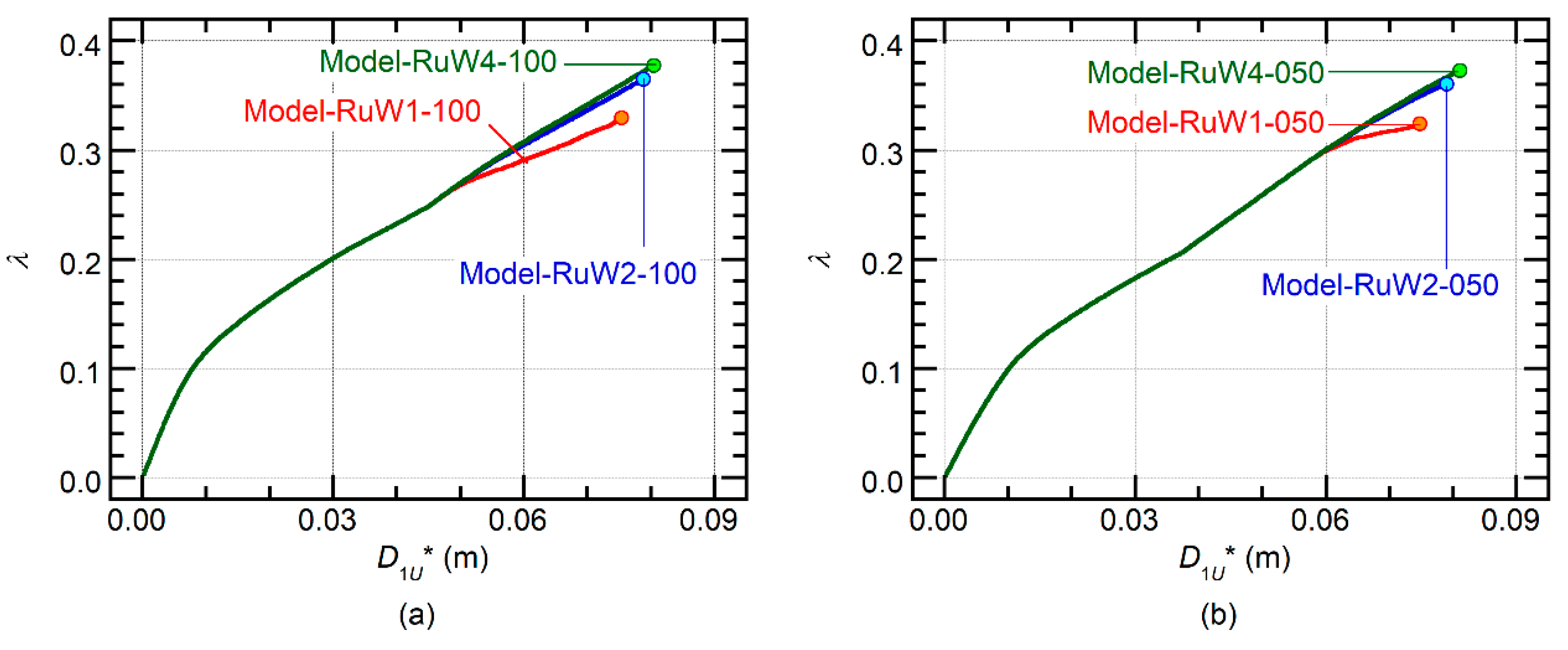
| Model ID | Displacement Limit | Capacity Index | ||||
|---|---|---|---|---|---|---|
| D1U*uni (×10−2 m) | D1U*bi (×10−2 m) | D1U*bi/D1U*uni | CI, uni | CI, bi | CI, bi/CI, uni | |
| RuW1-100 | 8.420 | 7.547 | 0.896 | 0.361 | 0.330 | 0.914 |
| RuW2-100 | 8.760 | 7.880 | 0.900 | 0.393 | 0.365 | 0.929 |
| RuW4-100 | 9.025 | 8.045 | 0.891 | 0.412 | 0.378 | 0.917 |
| RuW1-050 | 8.616 | 7.480 | 0.868 | 0.356 | 0.324 | 0.910 |
| RuW2-050 | 9.175 | 7.900 | 0.861 | 0.397 | 0.361 | 0.909 |
| RuW4-050 | 9.560 | 8.100 | 0.847 | 0.419 | 0.373 | 0.890 |
© 2019 by the author. Licensee MDPI, Basel, Switzerland. This article is an open access article distributed under the terms and conditions of the Creative Commons Attribution (CC BY) license (http://creativecommons.org/licenses/by/4.0/).
Share and Cite
Fujii, K. Pushover-Based Seismic Capacity Evaluation of Uto City Hall Damaged by the 2016 Kumamoto Earthquake. Buildings 2019, 9, 140. https://doi.org/10.3390/buildings9060140
Fujii K. Pushover-Based Seismic Capacity Evaluation of Uto City Hall Damaged by the 2016 Kumamoto Earthquake. Buildings. 2019; 9(6):140. https://doi.org/10.3390/buildings9060140
Chicago/Turabian StyleFujii, Kenji. 2019. "Pushover-Based Seismic Capacity Evaluation of Uto City Hall Damaged by the 2016 Kumamoto Earthquake" Buildings 9, no. 6: 140. https://doi.org/10.3390/buildings9060140
APA StyleFujii, K. (2019). Pushover-Based Seismic Capacity Evaluation of Uto City Hall Damaged by the 2016 Kumamoto Earthquake. Buildings, 9(6), 140. https://doi.org/10.3390/buildings9060140